water Article
Seismic-Reliability-Based Optimal Layout of a Water Distribution Network Do Guen Yoo 1 , Donghwi Jung 1 , Doosun Kang 2 and Joong Hoon Kim 3, * 1 2 3
*
Research Center for Disaster Prevention Science and Technology, Korea University, Seoul 136-713, Korea;
[email protected] (D.G.Y.);
[email protected] (D.J.) Department of Civil Engineering, Kyung Hee University, Yongin-si, Gyeonggi-do 446-701, Korea;
[email protected] School of Civil, Environmental and Architectural Engineering, Korea University, Anam-ro 145, Seongbuk-gu, Seoul 136-713, Korea Correspondence:
[email protected]; Tel.: +82-2-3290-3316; Fax: +82-2-928-7656
Academic Editor: Helena Ramos Received: 18 November 2015; Accepted: 25 January 2016; Published: 3 February 2016
Abstract: We proposed an economic, cost-constrained optimal design of a water distribution system (WDS) that maximizes seismic reliability while satisfying pressure constraints. The model quantifies the seismic reliability of a WDS through a series of procedures: stochastic earthquake generation, seismic intensity attenuation, determination of the pipe failure status (normal, leakage, and breakage), pipe failure modeling in hydraulic simulation, and negative pressure treatment. The network’s seismic reliability is defined as the ratio of the available quantity of water to the required water demand under stochastic earthquakes. The proposed model allows no pipe option in decisions, making it possible to identify seismic-reliability-based optimal layout for a WDS. The model takes into account the physical impact of earthquake events on the WDS, which ultimately affects the network’s boundary conditions (e.g., failure level of pipes). A well-known benchmark network, the Anytown network, is used to demonstrate the proposed model. The network’s optimal topology and pipe layouts are determined from a series of optimizations. The results show that installing large redundant pipes degrades the system’s seismic reliability because the pipes will cause a large rupture opening under failure. Our model is a useful tool to find the optimal pipe layout that maximizes system reliability under earthquakes. Keywords: seismic reliability; water distribution system; optimal layout; Anytown network
1. Introduction An earthquake occurs as a result of a sudden release of energy in the earth’s crust. The released massive energy creates seismic waves, which cause deformation of the water distribution system (WDS) of which components are mainly connected beneath the ground. The damage of an earthquake is the multiple failure of system components. For example, for an earthquake occurred in Kobe, Japan in 1995, many pipes were ruptured, causing water to flow out of the system, while some of the pump stations stopped working completely due to power outage. However, the likelihood of concurrence of multiple failures within a system is low under normal conditions. Therefore, a different strategy should be adopted for WDS design of the regions with the risk of earthquake occurrence, such as Japan, Korean peninsula, and West Coast cities of the United States. During the last two decades, many optimal design approaches have been proposed for WDSs. The early works have mainly taken into account the economic cost as a single objective [1–5]. Thereafter, some studies have included the system’s performance index within the optimization framework. Lansey et al. [6] developed a chance-constrained least-cost model in which the capacity reliability is Water 2016, 8, 50; doi:10.3390/w8020050
www.mdpi.com/journal/water
Water 2016, 8, 50
2 of 17
defined as the probability that stochastic pressures are equal to or higher than pressure requirement and are constrained at a certain level while minimizing cost. The nodal demands, pressure requirements, and pipe roughness coefficients were assumed to be uncertain while optimizing the pipe size. Several later studies also used chance-constrained optimization models for WDS design [7,8]. Kapelan et al. [9] was one of the earliest studies that proposed the multi-objective optimal design of WDS. Since then, most design approaches have adopted two objective functions to minimize economic cost and to maximize system reliability [10,11]. The various system reliability indices were suggested to reflect the uncertainties of pipe roughness and system demands when sizing the system. Component failures have been rarely considered in this stream of optimal WDS design. Su et al. [12] is one of the few studies that considered component failure in WDS design. In their study, reliability was defined as the probability of water demand provision under pipe break (failure) conditions and is used as a constraint for the least-cost design of a WDS. The minimum cut-set (i.e., the most critical set of pipes) was identified by closing the pipe individually for calculating the system reliability. Note that the pipe failure conditions were not considered in hydraulic simulation within the optimization framework, since the computational intensity is overwhelming. The seismic hazard assessment models have been developed recently. HAZUS [13] was the first model to assess the economic losses of an infrastructure by earthquake. HAZUS is mainly intended to assess the seismic damage but not detailed simulation of the system behavior. Later, the Mid-America Earthquake Center developed a seismic impact assessment model and investigated interdependencies between water and power systems [14]. Early earthquake studies in the water domain focused on investigating individual components’ physical behavior under earthquakes rather than quantifying the system-wide performance by modeling the WDS and earthquakes [15–17]. In a recent study, Fragiadakis et al. [18] proposed a seismic reliability assessment model of a WDS using survival curves of pipes based on general seismic assessment standards and American Lifelines Alliance (ALA) [19] guidelines. However, detailed hydraulic simulations were not conducted in this paper. Later studies began proposing methodologies to evaluate seismic reliability with hydraulic simulations using well-known hydraulic solvers and seismic simulations [20–29]. The latest and most popular assessment model is the graphical iterative response analysis for flow following earthquakes (GIRAFFE [30]) developed by a research team at Cornell University. GIRAFFE can simulate various pipe leakage and breakage conditions by using EPANET [31]. The model’s graphical user interface helps to visualize the model results, which is compatible with other geographic information system tools. After the initial development in 2008, the model has been improved and validated through many case studies [27,32–36]. However, GIRAFFE uses a controversial approach to treat negative pressure that removes the nodes’ negative pressure and connected pipes. This process is repeated until the negative-pressure nodes are no longer produced. This approach can be time-consuming because the system file must be revised iteratively. Yoo et al. [37] developed seismic reliability assessment model under stochastic earthquake events. The model quantifies the seismic reliability of a WDS through a series of procedures: stochastic earthquake generation, seismic intensity attenuation, determination of the pipe failure status (normal, leakage, and breakage), pipe failure modeling in hydraulic simulation, and negative pressure treatment. To the authors’ best knowledge, this study is the first attempt to develop an economic, cost-constrained optimal WDS design approach that takes into account seismic reliability based on detailed hydraulic simulations. The proposed model maximizes the system’s seismic reliability while satisfying the constraints on economic cost and node pressure requirements. The physical impacts of a seismic wave to WDS components are simulated to determine the failure conditions. The seismic reliability is defined as the ratio of the supplied water to the required demand under stochastic earthquake events. A well-known benchmark network, the Anytown network, is used for the applications of the optimal design and layout maximizing the seismic reliability.
Water 2016, 8, 50
3 of 17
Water 2016, 8, 50
3 of 16
2. Methodology 2. Methodology In reliability-based WDS optimization approach is proposed. Figure Figure 1 shows1 In this thisstudy, study,a seismic a seismic reliability-based WDS optimization approach is proposed. the flowchart of the proposed WDS optimal design model which consists of two sub-models: seismic shows the flowchart of the proposed WDS optimal design model which consists of two sub-models: reliability estimation and optimization model. model. Seismic reliability estimation modelmodel (SREM) first seismic reliability estimation and optimization Seismic reliability estimation (SREM) generates stochastic earthquake events by using earthquake generation module. Here, the locations first generates stochastic earthquake events by using earthquake generation module. Here, the and magnitude of stochasticofearthquakes are determined peak ground (PGA) reached locations and magnitude stochastic earthquakes areand determined andacceleration peak ground acceleration at each pipe is calculated in Section(described 2.1). Note that no hydraulic calculation is performed (PGA) reached at each (described pipe is calculated in Section 2.1). Note that no hydraulic from this module. This module also determines the failure mode of pipe where each pipe is classified calculation is performed from this module. This module also determines the failure mode of pipe as normal, leakage, or breakage (Section 2.2). where each pipe is classified as normal, leakage, or breakage (Section 2.2).
Seismic Reliability Estimation Model Earthquake Generation Module
(EPANET is not used)
Hydraulic Calculation Module
(EPANet is used)
Seismic Reliability Calculation Module
Optimization Model (Harmony Search Algorithm) Figure 1. 1. Flowchart Flowchart of of the the proposed proposed water water distribution distribution system system (WDS) (WDS) optimal optimal design design model. model. Figure
The failure modes are transferred to hydraulic calculation module where nodal pressures The failure modes are transferred to hydraulic calculation module where nodal pressures under under the failure conditions (i.e., the boundary conditions to the WDS system equation) are the failure conditions (i.e., the boundary conditions to the WDS system equation) are calculated calculated (Figure 1 and Section 2.3). Pipe leakage and breakage are modeled by the emitter in (Figure 1 and Sectionto2.3). Pipe leakagethe andconditions, breakage are modeled by the emitter in EPANET. In order EPANET. In order better simulate a semi pressure-driven analysis (semi-PDA) is to better simulate the conditions, a semi pressure-driven analysis (semi-PDA) is proposed. After an proposed. After an initial run of EPANET (a hydraulic simulator for DDA), the negative-pressure initial of EPANET (a zero, hydraulic simulator the(Section negative-pressure nodes’ demand is set to nodes’run demand is set to and the secondfor runDDA), is made 2.4). zero, The and the second run is made (Section 2.4). resulting hydraulics are provided to seismic reliability calculation module to quantify The resulting are provided seismic reliabilitysupply calculation module to quantify seismic reliability hydraulics which is defined as thetoratio of available to the required demandseismic under reliability is defined as the of available the required under stochastic which earthquake events. Theratio proposed WDS supply optimalto design modeldemand maximizes thestochastic system’s earthquake events. proposed optimal modelrequirements maximizes the system’s seismic reliability withThe constraints onWDS economic cost design and pressure (Figure 1 andseismic Section reliability with constraints on economic cost and pressure requirements (Figure 1 and Section 2.5). 2.5). Harmony search algorithm (HSA) is used for optimization (Figure 1) [38,39]. In the last section Harmony search algorithm (HSA) used for optimization (Figure 1)This [38,39]. In theislast section of the Methodology, Todini [40]’sisresilience indicator is defined. indicator not used of in the the Methodology, Todini [40]’s resilience indicator is defined. This indicator is not used in the proposed proposed model but used for a postoptimization analysis. model butfollowing used for a postoptimization analysis. The subsections describe the details of the methodology, such as earthquake The following subsections describe the details of the methodology, such as earthquake simulation, objective function, optimization approach, and semi-PDA method. Notesimulation, that the objective function, optimization approach, and semi-PDA method. Note that the following subsections following subsections are in the order that Figure 1 represents. are in the order that Figure 1 represents. 2.1. Earthquake Intensity Attenuation 2.1. Earthquake Intensity Attenuation The proposed model considers the physical characteristics of the WDS’s components to The proposed model considers the physical characteristics of the WDS’s components to determine determine the failure modes given earthquake intensity. Therefore, supplemental information such the failure modes given earthquake intensity. Therefore, supplemental information such as the types as the types of pipes and surrounding soil characteristics should be provided. Network information of pipes and surrounding soil characteristics should be provided. Network information such as the such as the network layout, nodal demands and coordinates, pipe diameters and lengths, and sizes network layout, nodal demands and coordinates, pipe diameters and lengths, and sizes of the pump of the pump and tanks are entered from the EPANET input file. The nodal coordinates are used to and tanks are entered from the EPANET input file. The nodal coordinates are used to calculate the calculate the location of a pipe that is used for calculating the distance from the epicenter. location of a pipe that is used for calculating the distance from the epicenter. Earthquake intensity is attenuated as it travels from the epicenter. In the model, three attenuation equations were adopted to quantify the damped energy of seismic waves. Kawashima et al. [41] relates the distance from the epicenter and earthquake magnitude to PGA (cm/s2) based on the 90 earthquakes that have occurred in Japan as
Water 2016, 8, 50
4 of 17
Earthquake intensity is attenuated as it travels from the epicenter. In the model, three attenuation equations were adopted to quantify the damped energy of seismic waves. Kawashima et al. [41] relates the distance from the epicenter and earthquake magnitude to PGA (cm/s2 ) based on the 90 earthquakes that have occurred in Japan as PGA “ 403.8 ˆ 100.265M ˆ pR ` 30q´1.218
(1)
where M = earthquake magnitude (e.g., M7 stands for earthquake magnitude 7), and R = the distance from the epicenter (km). Lee and Cho [42] presented a similar PGA function that was developed using the historical data of South Korea as log PGA “ ´1.83 ` 0.386M ´ logR ´ 0.0015R (2) Instead of using the horizontal distance from the epicenter, Baag et al. [43] relate the Euclidean distance from focus (∆) and earthquake magnitude to PGA as lnPGA “ 0.40 ` 1.2M ´ 0.76ln∆ ´ 0.0094∆
(3)
The average of the three calculated PGAs (from Equation (1) to Equation (3)) was used in our model. 2.2. Determination of Pipe Failure Mode The fragility of the pipes was determined based on the pipe repair rate (RR, number of pipe repairs/km) and the PGA. In this study, the RR equation suggested by Isoyama et al. [44] and adopted by ALA [19] was used. Isoyama et al. related the RR to the PGA by multiplying some correction factors denoting the pipe types, diameters and soil characteristics (Table 1) as RR “ C1 ˆ C2 ˆ C3 ˆ C4 ˆ 0.00187 ˆ PGA
(4)
where C1, C2, C3, and C4 represent the correction factors according to the pipe diameter, pipe material, topography, and soil liquefaction, respectively. Because of the lack of information, this study only considered the correction factor of the pipe diameter, C1, in Equation (4), while assuming other correction factors are equal to one. As seen in Table 1, for the smaller pipe, C1 increases and results in the higher probability of damage given the same PGA. Table 1. Correction factors (Isoyama et al. [44]). Category
Correction Factor
Pipe diameter (mm) (C1)
D < 100 100 ď D < 200 200 ď D < 500 500 ď D
1.6 1.0 0.8 0.5
Pipe material (C2)
Asbestos-Cement Pipe Poly-Vinyl Chloride Pipe, Vent Pipe Cast Iron Pipe Poly-Ethylene Pipe, High Impact (3-Layer) Pipe Steel Pipe Ductile Cast Iron Pipe
1.2 1.0 1.0 0.8 0.3 0.3
Topography (C3)
Narrow Valley Terrace Disturbed Hill Alluvial Stiff Alluvial
3.2 1.5 1.1 1.0 0.4
Liquefaction (C4)
Total Partial None
2.4 2.0 1.0
Water 2016, 8, 50
5 of 17
The post-earthquake pipe status was classified into normal, leakage, or breakage conditions. Pipe leakage is defined as a small rupture on the pipe wall or at the joint through which continuous minor water loss occurs. Pipe breakage is defined as a complete separation of the pipe into two pieces that causes complete loss of transportation ability. ALA [19] suggested that the probability of pipe breakage (Pfbreakage,i ) is a function of the RR and the length of the pipe (Li , km) expressed as Pfbreakage,i “ 1 ´ e´RRˆLi
(5)
As a rule of thumb, the probability of pipe leakage (Pfleakage ,i ) is assumed to be five times higher than the probability of pipe breakage [19]. If the cumulative probability of the two conditions is less than 1.0 (e.g., Pfbreakage,i = 0.1 and Pfleakage,i = 0.5), the complementary probability is assigned for the normal condition (Pnormal = 0.4). However, if the cumulative probability of the leakage and breakage is greater than 1 (e.g., Pfbreakage,i = 0.18 and Pfleakage,i = 0.90), the model assumes that the normal condition (without any damage) is not available, and the two failure probabilities are normalized to make the sum of 1.0 (Pfbreakage,i = 0.18/(0.18 + 0.90) = 0.17 and Pfleakage,i = 0.90/(0.18 + 0.90) = 0.83). 2.3. Pipe Failure Modeling Once the status of each pipe is determined, the information is entered into a network solver, EPANET, for hydraulic simulation (i.e., solving for WDS system equations consisting of conservations of mass and energy). To simulate the pipe leakage, pressure-dependent flows (Ql ) are assigned to the closest node to the damaged pipe using the following equation: Ql “ CD pα
(6)
˙ 2g α where CD = the discharge coefficient (= A) (the emitter coefficient in EPANET), where γw g = gravitational acceleration and α = the exponent of the power function; γw = the specific weight of water; A = the opening area of the damaged pipe; and p = pressure at the closest node. Lambert [45] conducted an experimental study to investigate the accuracy of the power function model in Equation (6) and provided a guideline on using exponent α based on the pipe material and level of leakage. It was suggested that the exponent of 0.5 would be used to simulate large detectable leakages in metal pipes; the exponent of 1.0 (linear relationship between discharge and pressure) would be used if no information on the pipe material is available. Puchovsky [46] theoretically derived a discharge coefficient and validated it using sprinkler data. The shape and area of the opening on ruptured pipe varies depending on pipe material, origin of the pipe damage, and direction of external force. Large opening area is more likely to occur in the failure of large pipes than smaller pipes. To that end, it was assumed that the total opening area is equivalent to 10% of the entire cross-sectional pipe area during leaks. In case of breakage, the entire cross-sectional area was used as the opening area. If a pipe was tagged as leaking, it was modeled in a hydraulic simulation, as illustrated in Figure 2a, and the discharge coefficient was assigned to the downstream node. The pipe breakage was modeled as shown in Figure 2b. The discharge coefficient was assigned to the upper node in flow direction. Then, the broken pipe was set to “closed” to disconnect the water flow. The demand of the node connected to a broken pipe was modified to consider the degraded delivery capacity due to disconnection. In the model, the nodal demands of both end junctions of the broken pipe were reduced by degrees of node (DoN). Here, DoN is defined as the number of connections/edges that a node has to other nodes in a network. As shown in Figure 2b, the base demand of the upstream node is reduced by 25% (= 1/DoN = 1/4), while the downstream node is reduced by 33.3% (= 1/DoN = 1/3). ˆ
Water 2016, 8, 50
Water 2016, 8, 50
6 of 17
6 of 16
Figure 2. A2.schematic diagram to describe pipe damage and (b) Figure A schematic diagram to describe pipe damagemodeling: modeling: (a) (a)leakage leakage condition condition and breakage condition. (b) breakage condition.
2.4. Negative Pressure Treatment 2.4. Negative Pressure Treatment Hydraulic analysis approaches waterdistribution distribution network network can a DDA and Hydraulic analysis approaches forforwater canbe beclassified classifiedasas a DDA and a a pressure-driven analysis (PDA). DDA assumes that the demand at individual node is satisfied pressure-driven analysis (PDA). DDA assumes that the demand at individual node is satisfied regardless of the associated pressure,while whilePDA PDA assumes assumes that is dependent on the regardless of the associated pressure, thatnodal nodaldischarge discharge is dependent on the pressure head expressed by the head-outflow relationship (HOR). DDA often generates negative pressure head expressed by the head-outflow relationship (HOR). DDA often generates negative pressure when simulating abnormal conditions, such as multiple pipe breaks. PDA, on the other hand, pressure when simulating abnormal conditions, such as multiple pipe breaks. PDA, on the other provides more realistic hydraulics avoiding negative pressures. WaterGEMS [47], WDNetXL [48], and hand,WaterNetGen provides more hydraulics avoiding negativewith pressures. WaterGEMS WDNetXL [49]realistic are well-known programs equipped PDA option based on[47], HOR. However,[48], and the WaterNetGen [49] areshould well-known programs with PDA option based HOR. system-specific HOR be provided, which isequipped spatially and temporally inconsistent andon also However, the dependent. system-specific HOR be provided, which is spatially temporally operational Therefore, forshould PDA techniques used in pipe network analyses,and the analyzer inconsistent and also operational dependent. for PDA states techniques in pipe network should assume a HOR for the whole network.Therefore, Given that hydraulic of pipeused networks can vary greatly with changesshould in HORs, analysis resultsfor cannot guarantee high accuracy. analyses, the analyzer assume a HOR the whole network. Given that hydraulic states of Quasi-PDA methods suppress occurrence of negative pressure through repetitive DDAhigh pipe networks can vary greatly withthe changes in HORs, analysis results cannot guarantee analyses. In general, if negative pressure occurs from the first DDA run, better hydraulic calculation accuracy. results can bemethods derived suppress through quasi-PDA methods by resetting the nodal demands and theDDA Quasi-PDA the occurrence of negative pressure through repetitive components’ status. analyses. In general, if negative pressure occurs from the first DDA run, better hydraulic calculation Ballantyne et al. [21] used the KYPIPE model [50] for hydraulic analyses. KYPIPE, a DDA program results can be derived through quasi-PDA methods by resetting the nodal demands and the similar to EPANET, can also produce negative pressures during simulation of pipeline destruction. components’ Ballantynestatus. et al. calculated system reliability by assuming that water could not be supplied to points Ballantyne al. [21] but used KYPIPE model [50] hydraulic analyses. a DDA with negativeetpressures, thethe hydraulic results around thefor negative-pressure node stillKYPIPE, did not have program similar EPANET, also produce pressures during simulation of pipeline realistic values.toThe method ofcan Shinozuka et al. [22]negative and Shi [27] completely removed negative-pressure destruction. et pipelines al. calculated system bythe assuming that water could not be nodes andBallantyne the connected from the originalreliability network, but process required time-consuming repetitive hydraulic and regeneration input files. supplied to points withanalyses negative pressures, butofthe hydraulic results around the negative-pressure node still did not have realistic values. The method of Shinozuka et al. [22] and Shi [27] completely removed negative-pressure nodes and the connected pipelines from the original network, but the process required time-consuming repetitive hydraulic analyses and regeneration of input files. Here, a quasi-PDA approach is proposed for realistic hydraulic simulation under multiple failure conditions to avoid the occurrence of negative pressure. That is, if negative pressure occurred after DDA simulation using EPANET, the updated base demand (after modification
Water 2016, 8, 50
7 of 17
Here, a quasi-PDA approach is proposed for realistic hydraulic simulation under multiple failure conditions to avoid the occurrence of negative pressure. That is, if negative pressure occurred after DDA simulation using EPANET, the updated base demand (after modification described in Chapter 2.3) of the negative-pressure node is set to zero and DDA is repeated. If negative pressure reappears, the pressure of the relevant node is assumed to zero. Compared to Shinozuka et al. [22] and Shi [27] approach, the proposed approach saves overhead processing time by avoiding regeneration of the EPANET input file for the new configuration. In addition to the negative pressure treatment, pressure-dependent water supply is considered in calculating the quantity of available water at each node. The available nodal demand at node j (Qavl,j ) is estimated as $ ’ ’ ’ & Qavl,j “
0d Qnew,j ˆ
’ ’ ’ %
Qnew,j
if Pj ď 0 Pj Pmin
if 0 ă Pj ă Pmin
(7)
if Pj ě Pmin
where Qnew,j = the updated base demand with pipe breakage consideration and negative pressure treatment at node j; Pj = the pressure head at node j; and Pmin “ the minimum pressure requirement. 2.5. Seismic Reliability Indicator Various surrogate measures of WDS reliability have been proposed including capacity reliability [6,7], resilience [40], robustness [10,11], availability [51]. Bao and Mays [52] proposed three formulations of WDS system reliability which can be calculated from nodal reliability values: minimum nodal reliability, arithmetic mean reliability, and flow-weighted mean reliability. The first one concerns on the worst nodal reliability while the latter two values indicate system-wide reliability. In order to represent post-earthquake system performance in the water supply, a seismic reliability measure should be able to reflect system-wide water availability rather than local level of system performance. To quantify system-wide seismic reliability, a new reliability indicator is proposed herein. The system seismic reliability (SS ) is defined as the ratio of the total available system demand to the total required system demand: řm j“1 Qavl,j (8) SS “ řm j“1 Qreq, j where m = total number of demand nodes; and Qreq,j = the required demand at node j. A water system planner would intend to design the most reliable network for earthquakes under a given budget condition. To that end, the proposed model here is a single-objective optimal design model that maximizes the system’s seismic reliability with a constraint on economic cost. The optimization model is formulated as follows: Maximize F “ Ss s.t.CC ď CCgiven
(9)
where CC = the pipe construction cost; CCgiven = the available budget for pipe system. Equation (9) is valid for each set of available commercial pipe diameters and in conditions where the minimum pressure head is guaranteed. The pipe construction cost accounting for the pipe material and installation is expressed as: n ÿ CC “ puc pDi q ˆ Li q (10) i “1
where uc pDi q = the unit cost of the pipe with diameter Di determined for the ith pipe (USD/m); and Li = the length of the ith pipe.
Water 2016, 8, 50
8 of 17
2.6. Resilience Indicator In this study, Todini [40]’s resilience is quantified from a range of designs of the Anytown network and compared with seismic reliability. Todini [40] introduced a resilience index to quantify the resilience of looped network. Resilience is defined as surplus power available within the network as a percentage of net input power as: řm
` ˘ Qreq,j Hj ´ Hreq Resil “ řnr řnp Poweri řm ´ j Qreq,j Hreq k“1 Qk Hk ` i“1 γ j
(11)
where Hj = total head of the jth node; Qk = flow provided by reservoir k (m3 /s); Hk = head at reservoir k; Poweri = power of the ith pump (Nm/s); γ = specific weight of water (N/m3 ); nr and np = number of reservoir and pumps, respectively. Note that this indicator was used only for a postoptimization analysis. Todini’s resilience is one of the most popular and widely used surrogate measures of WDS reliability. Farmani et al. [53] investigated the trade-off between economic cost and the resilience for a rehabilitation problem of the Anytown network. Prasad and Park [54] proposed a multiobjective optimization approach to minimize cost and maximize modified version of Todini’s resilience indicator. Recently, Gheisi and Naser [55] compared entropy-based reliability, Todini’s resilience, and three modified versions of Todini’s resilience in the twenty-two potential pipe layouts of a hypothetical network. 3. Study Network The proposed optimization approach is applied for optimal design of a well-known benchmark WDS, the Anytown network. The network, which was firstly published by Walski et al. [56], was modified by Jung et al. [11] for pipe only and pipe/pump designs that minimize total cost and maximize system robustness. The original benchmark network was modified by removing the two tanks and the connected riser pipes to be solely supplied by a single reservoir with a fixed source head. The fixed source head is elevated from 3 m (10 ft) to 73.2 m (240 ft). A peaking factor of 1.8 is applied to given average-based demand (2005 average daily use) to create the daily peak condition. Other modifications of the study network were made for application purposes. First, this study suggests new pipe layouts and sizes assuming there are no existing pipes in the system. Pump and tank design are not considered. Second, in addition to 10 commercial pipe sizes (152, 203, 254, 305, 356, 406, 457, 508, 610, and 762 mm), zero diameter can be selected suggesting no pipe installation for the potential path. The unit costs of the commercial pipes are adopted from Walski et al. [56]. To generate random epicenters, a 2 ˆ 2 grid was created and laid on the study network as seen in Figure 3. The rectangular boundary of the grid is defined by the four end nodes: north, south, east, and west. Total 900 earthquakes are generated and consistent number of earthquakes are assigned at each corner of the grid (marked as “x” in Figure 3). The earthquake intensity reached at the pipe is a function of the earthquake magnitude and the Euclidean distance from the epicenter. Note the earthquake magnitude of M4 was generated from each corner of the grid. The minimum pressure requirement of 28.12 m (40 psi) should be satisfied under based demand condition and is also considered in Equation (7).
and west. Total 900 earthquakes are generated and consistent number of earthquakes are assigned at each corner of the grid (marked as “x” in Figure 3). The earthquake intensity reached at the pipe is a function of the earthquake magnitude and the Euclidean distance from the epicenter. Note the earthquake magnitude of M4 was generated from each corner of the grid. The minimum pressure requirement also Water 2016, 8, 50 of 28.12 m (40 psi) should be satisfied under based demand condition and is9 of 17 considered in Equation (7).
Figure 3. Study network layout (epicenter is marked as “x”). Figure 3. Study network layout (epicenter is marked as “x”).
HSA was used to find an optimal solution for the pipe sizing problem. HSA was inspired by musical performance process and widely used for WDS optimizations. While the applications encompass from pipe network design to pump scheduling, HSA was proven to be generally outperform other algorithms such as genetic algorithm [57–59]. Several assumptions and simplifications were made in this study: (1) the seismic damages of the pump, tank, reservoir, and valve are not considered; (2) the earthquake’s focal depth (tectonics) is assumed to be 10 km; (3) the coordinate of the center of the pipe is used as a reference point for calculating the distance from the epicenter; (4) Pipes are cast iron pipes; and (5) the Anytown network is laid on the alluvial plain with no liquefaction. Based on the assumption (4) and (5), all correction factors except C1 in the Equation (4) (C2-4) are equal to one. 4. Application Results First, we applied two different commercial pipe sets for the pipe sizing of the study network. This analysis investigates the WDS’s layout changes with respect to the seismic reliability increase. The same total cost constraint was applied for the two designs and the resultant pipe layouts were compared. Then, seven designs with a fixed layout and different redundancy levels were compared for the systems’ seismic reliability. Finally, discussions and suggestions on improving WDS seismic reliability were provided at the end of this section. 4.1. Different Available Pipe Sizing Options The first application is intended to investigate the impact of seismic reliability on the network’s layout. Two sets of commercial pipe sizes are assumed to be available for two design cases. In Case 1, all commercial pipes (152, 203, 254, 305, 356, 406, 457, 508, 610, and 762 mm) except the zero size option are available. In Case 2, zero diameter is available in addition to the commercial sizes in Case 1. Considering the same cost constraint (CCgiven = 18 million (M) USD) in Equation (9) provided a platform for consistent comparison of the resulting designs. Figure 4 shows the optimal seismic reliability values of the two case designs. The corresponding optimal pipe layouts are presented in Figure 5. Contrary to expectations, the seismic reliability decreased with the availability of more pipe sizes. In Case 1, at least a 152 mm pipe should be installed because no pipe option is not available. By comparing Figures 5a,b and 6, we can observe that 152 mm pipes were installed in Case 1 for the link at which no pipe was constructed in Case 2. The 152 mm pipe, which is the most vulnerable pipe to earthquakes, almost always causes failure. Being able to have no pipe instead of a 152 mm pipe increased the system’s seismic reliability by 0.2 (a 20% increase
optimal pipe layouts are presented in Figure 5. Contrary to expectations, the seismic reliability decreased with the availability of more pipe sizes. In Case 1, at least a 152 mm pipe should be installed because no pipe option is not available. By comparing Figure 5a,b and Figure 6, we can observe that 152 mm pipes were installed in Case 1 for the link at which no pipe was constructed in 2. 50 The 152 mm pipe, which is the most vulnerable pipe to earthquakes, almost always causes Water Case 2016, 8, 10 of 17 failure. Being able to have no pipe instead of a 152 mm pipe increased the system’s seismic reliability by 0.2 (a 20% increase in the amount of available water during an earthquake). The network layout becomes smaller from Case 2 toduring Case 1 (Figure 5a,b), whileThe the network overall pipe diameters also smaller increase from in the amount of available water an earthquake). layout becomes 6). 1 (Figure 5a,b), while the overall pipe diameters also increase (Figure 6). Case(Figure 2 to Case
Figure 4. Maximum seismicreliability reliabilityvalues values of with different pipepipe sizing options. Figure 4. Maximum seismic of two twocase casedesigns designs with different sizing options.
Note that this is very different from what we observed in a traditional capacity reliability-based
Note that this is very different from what we observed in a traditional capacity reliability-based design. In the context of the capacity reliability field, it was believed that having additional paths and more loopsloops would result in the of system reliability and redundancy and more would result in increase the increase of system reliability and redundancy[11,60]. [11,60].However, However,the the Water 2016, 8, 50 10 of 16 result of this study indicates that a different strategy should be available under the conditions where result of this study indicates that a different strategy should be available under the conditions where WDS component are affected by strong external forcesand (i.e., earthquakes) andHowever, the components’ WDS component failures are affected by strong external forces (i.e.,[11,60]. earthquakes) and the and more loopsfailures would result in the increase of system reliability redundancy the physical characteristics (pipe’s probability of failure as a function of RR). result of this study indicates that a different strategy should be available under the conditions where components’ physical characteristics (pipe’s probability of failure as a function of RR). Waterdesign. 2016, 8, In 50 the context of the capacity reliability field, it was believed that having additional paths10 of 16
WDS component failures are affected by strong external forces (i.e., earthquakes) and the components’ physical characteristics (pipe’s probability of failure as a function of RR). 152
Diameter
Diameter
1.00
200.00
700.00
Diameter
mm
1.00
203
203
200.00
152 610 152
762
762
152
152
762
508 203
305
152
762 508
(a) Case 1
762
508 508
254
2540 2540
610 610 0
762
762
0
508
0
0
0
406
406
762
508
254
356 356
762 762
508
762
762
0
0
0
254
0
762
762 0
0
0
0
0
508
508 508
0
0
305
762 762 305
254
762
762 762
508
762
762
762
356 0
152
305 0
762
356
203
508
203
762
508 508
203
203
0 0
0 508
0
0
762
508
152203
305
mm
610
0
0
203
152
305
762
700.00
508
203 254
762
305 203
203 203 508
610
203 152
762
152
152
254
762
203
0
0
203
152
254
305
508
500.00
610
762
762
1.00 mm
203
254
mm
203
610
0
Diameter 700.00
508
152
508
305
152
152
610
500.00
305
200.00 500.00
200.00
700.00
508
1.00
508
508
500.00
762
2540
762 762
2540
(b) Case 2
(a) Case 1 (b) Case 2 Figure 5. Pipe layout comparison for the solutions obtained from Cases 1 and 2 (Figure 4); pipe Figure 5. Pipe layoutcomparison comparison for for the the solutions from Cases 1 and 2 (Figure 4); pipe Figure 5. Pipe layout solutionsobtained obtained from Cases 1 and 2 (Figure 4); pipe diameters are in mm; the thicker and darker pipe is larger. (a) Case 1; (b) Case 2. diameters in mm; thickerand anddarker darker pipe pipe is 1; (b) Case 2. 2. diameters are are in mm; thethe thicker islarger. larger.(a) (a)Case Case 1; (b) Case
Figure 6. Histogram of pipes by the pipe diameter. Figure 6. Histogram of pipes by the pipe diameter.
Figure 6. Histogram pipes byinthe diameter. This plateau in seismic reliability was also of observed thepipe optimal pipe designs of the Anytown network by applying different total cost constraints and using the available pipe sizes in Case 1. This plateau seismic was alsototal observed in the optimal pipe designs of the cost Anytown Figure 7 showsinthe Paretoreliability optimal solutions’ cost and seismic reliability. The marginal network by applying different total cost constraints and using the available pipe sizes in Case 1. becomes infinite for the designs whose cost is greater than 16.5 M USD. A reliability increase can no Figure 7 shows the Pareto costAlthough and seismic reliability. longer be achieved once a optimal sufficient solutions’ investment total is made. the designs greaterThe thanmarginal 16.5 M cost
Water 2016, 8, 50
11 of 17
This plateau in seismic reliability was also observed in the optimal pipe designs of the Anytown network by applying different total cost constraints and using the available pipe sizes in Case 1. Figure 7 shows the Pareto optimal solutions’ total cost and seismic reliability. The marginal cost becomes infinite for the designs whose cost is greater than 16.5 M USD. A reliability increase can no longer be achieved once a sufficient investment is made. Although the designs greater than 16.5 M USD have more large pipes compared to the solutions less than 16.5 M USD (the number of pipes equal to or larger than 508 mm is between 7 and 10, while the designs less than 16.5 M USD have three to five pipes), no benefit of having larger pipes was obtained with respect to seismic reliability. For effective and economical improvement of WDS seismic reliability, the threshold investment for a network should first be identified. Water 2016, 8, 50 Water 2016, 8, 50
11 of 16
11 of 16
Figure 7. 7. Trade-off and seismic seismic reliability reliabilityininCase Case1 1where where all pipes Figure Trade-offrelationship relationshipbetween between total total cost and pipes Figure 7. Trade-off relationship between total cost and seismic reliability in Case 1 where all all pipes (152, (152, 203, 254, 305, are available availableand andwithout withoutzero zero pipe option. (152, 203, 254, 305,356, 356,406, 406,457, 457,508, 508,610, 610,and and 762 762 mm) are pipe option. 203, 254, 305, 356, 406, 457, 508, 610, and 762 mm) are available and without zero pipe option.
Constant Layoutwith witha aSingle SinglePipe PipeSizing Sizing Option Option 4.2.4.2. Constant Layout 4.2. Constant Layout with a Single Pipe Sizing Option Theimpacts impactsofofhaving having large large pipes pipes are are also also investigated The investigated through throughthe theseismic seismicreliability reliability The impacts of having large pipes are also investigated through the seismic reliability evaluation evaluation of seven uniform designs. The Design 1 has 305 mm for all pipes in the study network. evaluation of seven uniform designs. The Design 1 has 305 mm for all pipes in the study network. of seven uniform designs. The Design 1 has 305508, mm610, for and all pipesmm, in the study network. Design 2, 3, 4, Design and7 7have have 356,406, 406, 457, pipes. The Design 2, 2, 3, 3, 4, 4, 5, 5,6,6,and 356, 457, 508, 610, and 762 762 mm,respectively, respectively,forforallall pipes. The 5, 6, and 7 reliabilities have 356, 406,the 457, 508,designs 610, andare 762 mm, in respectively, for all pipes. The seismic reliabilities seismic seven shown resilience is is seismic reliabilities ofofthe seven designs are shown in Figure Figure8.8.For Forcomparison, comparison,Todini’s Todini’s resilience of the seven designs arethe shown in designs Figure 8.and Forplotted comparison, Todini’s resilience is also calculated from also calculated from seven increase in in also calculated from the seven designs and plotted in in Figure Figure 8.8. While Whilethere thereisisa alarge large increase theseismic seven designs plotted in mm Figure 8. While there is athe large in seismic from reliabilityand from the 457 design (Design 4) to 508 increase mm design (Designreliability 5), reliability seismic reliability from the 457 mm design (Design 4) to the 508 mm design (Design 5), reliability thedecreases 457 mm design (Design 4)design to the to 508the mm (Design 5), reliability decreases from 508 mm from the 508 mm 762design mm design (Design 7). This explains why wethe observed decreases from the 508 mm design to the 762 mm design (Design 7). This explains why we observed a plateau seismic reliability in Figure 7. explains On the other hand, resilience (a traditional reliability design to thein 762 mm design (Design 7). This why we observed a plateau in seismic reliability a plateau in seismic reliability in Figure 7. On the other hand, resilience (a traditional reliability measure) consistently increases with (a increasing sizes. measure) The marginal cost ofincreases improving in Figure 7. On the other hand, resilience traditionalpipe reliability consistently with measure) consistently increases with increasing pipe sizes. The marginal cost of improving resiliencepipe increases substantially resilience value of 0.3–0.8 and stabilized for a value higher increasing sizes. The marginal for costa of improving resilience increases substantially for a resilience resilience increases substantially for a resilience value of 0.3–0.8 and stabilized for a value higher thanof0.8. value 0.3–0.8 and stabilized for a value higher than 0.8. than 0.8.
Figure Seismicreliability reliabilityofofthe theseven seven uniform uniform designs; designs; all Figure 8. 8. Seismic allpipes pipesare are508 508mm mmininCase Case5.5.
Figure 8. Seismic reliability of the seven uniform designs; all pipes are 508 mm in Case 5.
As the pipe sizes decrease, the correction factor for RR (Equation (4)) increases, finally resulting in high pipe breakage and leakage probability. However, although the pipes failed, the resulting As the pipe sizes decrease, the correction factor for RR (Equation (4)) increases, finally resulting impact is not significant to the system’s seismic reliability because the calculated discharge in high pipe breakage and leakage probability. However, although the pipes failed, the resulting coefficient, which is a function of the pipe’s cross-sectional area (Table 2), is not large. However, as impact is not significant to the system’s seismic reliability because the calculated discharge seen in Table 2, large pipes such as 508, 610, and 762 mm have a smaller failure probability
Water 2016, 8, 50
12 of 17
As the pipe sizes decrease, the correction factor for RR (Equation (4)) increases, finally resulting in high pipe breakage and leakage probability. However, although the pipes failed, the resulting impact is not significant to the system’s seismic reliability because the calculated discharge coefficient, which is a function of the pipe’s cross-sectional area (Table 2), is not large. However, as seen in Table 2, large pipes such as 508, 610, and 762 mm have a smaller failure probability compared to small pipes, but the resulting discharge coefficient is more than 10 times as big as that of small pipes. The failure effects are Water 2016, 8, 50 12 of 16 more significant for system seismic reliability compared to small pipes. Table2.2.Correction Correctionfactors factorsand anddischarge dischargecoefficients coefficients(Equation (Equation(6)) (6))for forthe thepipe pipesizes sizesconsidered. considered. Table Discharge Coefficient Pipe Sizes Pipe’s Correction Discharge Coefficient Pipe Sizes Cross-Sectional Correction Pipe’s Cross-Sectional Factor (C1) mm inch Breakage (100% of A) Leakage (10% of A) Breakage Leakage Area (A) Factor (C1) Area (A) mm inch (100% of A) (10% 152 6 28 1 1074 107of A) 203 8 6 50 0.8 1910 1074 191 152 28 1 107 203 50 0.8 191 254 10 8 79 0.8 2985 1910 298 254 0.8 298 305 12 10 113 79 0.8 4298 2985 430 305 0.8 430 356 14 12 154 113 0.8 5850 4298 585 356 0.8 585 406 16 14 201 154 0.8 7640 5850 764 406 16 201 0.8 7640 764 457 18 254 0.8 9670 967 457 18 254 0.8 9670 967 508 20 314 0.5 11,938 1194 508 20 314 0.5 11,938 1194 610 24 24 452 452 0.5 17,19117,191 1719 610 0.5 1719 762 30 707 0.5 26,861 2686 762 30 707 0.5 26,861 2686
4.3. Random Designs 4.3. Random Designs Finally, random designs that satisfy pressure requirements are generated from the proposed Finally, random designs that satisfy pressure requirements are generated from the proposed model to confirm the aforementioned conclusion. Figure 9 shows the profiles of seismic reliability model to confirm the aforementioned conclusion. Figure 9 shows the profiles of seismic reliability and resilience of many random designs. We can clearly see that there is an inflection point around and resilience of many random designs. We can clearly see that there is an inflection point around the the total cost of 23 M USD and seismic reliability around 0.4, after which the overall seismic total cost of 23 M USD and seismic reliability around 0.4, after which the overall seismic reliability reliability decreases (Figure 9a). Because the total cost is a direct function of the pipe diameter, this decreases (Figure 9a). Because the total cost is a direct function of the pipe diameter, this plot indicates plot indicates that installing large pipes does not always guarantee an increase in seismic reliability. that installing large pipes does not always guarantee an increase in seismic reliability. The printed The printed solutions are all suboptimal solutions that are dominated by the Pareto solutions found solutions are all suboptimal solutions that are dominated by the Pareto solutions found in Figure 7. in Figure 7. On the other hand, installing large pipes resulted in an upward trend in resilience On the other hand, installing large pipes resulted in an upward trend in resilience (Figure 8b). (Figure 8b).
(a)
(b)
Figure 9. (a) Seismic reliability of randomly generated solutions (black dot) and Pareto solutions Figure 9. (a) Seismic reliability of randomly generated solutions (black dot) and Pareto solutions shown in Figure 7 (blue diamond) and (b) resilience of the same random designs. shown in Figure 7 (blue diamond) and (b) resilience of the same random designs.
Under normal failure condition, having more additional paths and installing large pipes Under normal failure more additional and (i.e., installing pipes throughout the system arecondition, beneficial having with respect to system paths reliability abilitylarge to supply throughout the system are beneficial with respect to system reliability (i.e., ability to supply required required quantity of water) and redundancy (i.e., level of pressure redundancy). However, we quantity water) level of failures. pressureEarthquake redundancy). However, observed this observedofthis doesand not redundancy apply under(i.e., earthquake deforms WDSwe components and their original function. Once failed under earthquakes, large pipes, which can deliver large volume of water under normal condition, help accelerate water loss out of the system. This study was the first attempt to take into account such irregular hydraulic behavior in the WDS modeling and design and highlight the need to find the optimal pipe layout considering the system’s performances under the two different states.
Water 2016, 8, 50
13 of 17
does not apply under earthquake failures. Earthquake deforms WDS components and their original function. Once failed under earthquakes, large pipes, which can deliver large volume of water under normal condition, help accelerate water loss out of the system. This study was the first attempt to take into account such irregular hydraulic behavior in the WDS modeling and design and highlight the need to find the optimal pipe layout considering the system’s performances under the two different states. 5. Summary and Conclusions Earthquakes can cause many simultaneous failures of components throughout WDSs, which result in very different and severe conditions compared to normal failure conditions that water communities usually deal with (e.g., single pipe failure). In this study, an economic, cost-constrained optimal design approach of a WDS was proposed to maximize seismic reliability. The network’s seismic reliability is defined as the ratio of the available supply to the required water demand during stochastic earthquakes. The physical relationship between the earthquake intensity and the WDS components’ vulnerability characteristics was defined and utilized for quantifying seismic reliability. To overcome the limitation of DDA in modeling earthquake failures, negative pressures were assumed to have realistic hydraulic calculations. Then, we investigated the seismic reliability improvement with respect to the economic investment in the system and the associated topological and pipe diameter changes. A traditional benchmark network, the Anytown network, was used to demonstrate the approach. Random earthquakes around the study network were generated for reliability quantification. The results were quite different from what we generally observed from traditional reliability-based design (e.g., resilience-based design). First, allowing redundant small pipes in the system did not help improve seismic reliability. Those pipes cause frequent failures because of their low durability to earthquake forces. Second, having too-large pipes also degrades the system reliability during earthquakes. Compared to small pipes that are 152 mm to 305 mm, a big pipe (762 mm) has a lower failure probability; however, the failure’s influence is very significant to the system once it fails. The large pipe’s cross-sectional area will help release more water out of the system. Therefore, the first step to efficiently improve the WDS seismic reliability should be to identify the most appropriate pipe sizes for a system. For example, from the Anytown network, having a uniform 508 mm for all pipes provides the highest system reliability of 0.38 among seven uniform designs. This study has several limitations that future research must address. First, this model is sensitive to correction factors for the pipe and the assumption of the opening area of the pipe under failure. Intensive sensitivity analysis should be conducted with experimental studies to simulate the most realistic failure behavior of WDS components. Second, this study only considers the pipe failures while pump, valve, tank, and reservoir failure can occur during an earthquake. Therefore, various failure types could be included in future studies. The proposed semi-PDA approach and EPANet can be replaced with a PDA-based network solver in order to simulate more realistic behavior of WDS under earthquake events. Third, while this study focuses on the system’s reliability right after an earthquake occurs, post-earthquake recovery strategies should also be investigated to enhance the overall WDS’s reliability/resilience. This could be found mostly in the context of operation and management. Fourth, the proposed semi-PDA approach and EPANet can be replaced with a PDA-based network solver in order to simulate more realistic behavior of WDS under earthquake events. Finally, interdependencies among multiple lifeline infrastructures (e.g., the water, power, transportation, and communication systems) can help improve and recover an individual infrastructure’s reliability during an earthquake. Therefore, more efforts should be made to identify these interdependencies. Acknowledgments: This work was supported by a grant from The National Research Foundation (NRF) of Korea, funded by the Korean government (MSIP) (No. 2013R1A2A1A01013886) and the Korea Ministry of Environment as “The Eco-Innovation project (GT-11-G-02-001-2)”. Author Contributions: Do Guen Yoo and Donghwi Jung carried out the survey of previous studies, analysis of proposed method, participated in the sequence alignment and drafted the manuscript. Joong Hoon Kim and Doosun Kang conceived the original idea of the study, and helped to write the final manuscript.
Water 2016, 8, 50
14 of 17
Conflicts of Interest: The authors declare no conflicts of interest.
References 1.
2. 3. 4. 5. 6. 7. 8. 9. 10. 11. 12. 13. 14. 15. 16. 17. 18. 19. 20. 21. 22.
23.
Schaake, J.; Lai, D.D. Linear Programming and Dynamic Programming Applications to Water Distribution Network Design; Report No. 116; Department of Civil Engineering, Massachusetts Institute of Technology: Cambridge, MA, USA, 1969. Alperovits, E.; Shamir, U.U. Design of optimal water distribution systems. Water Resour. Res. 1977, 13, 885–900. [CrossRef] Lansey, K.; Mays, L. Optimization model for water distribution system design. J. Hydraul. Eng. 1989, 115, 1401–1418. [CrossRef] Simpson, A.; Dandy, G.; Murphy, L. Genetic algorithms compared to other techniques for pipe optimization. J. Water Resour. Plan. Manag. 1994, 120, 423–443. [CrossRef] Savic, D.; Walters, G. Genetic algorithms for least-cost design of water distribution networks. J. Water Resour. Plan. Manag. 1997, 123, 67–77. [CrossRef] Lansey, K.; Duan, N.; Mays, L.; Tung, Y. Water distribution system design under uncertainty. J. Water Resour. Plan. Manag. 1989, 115, 630–645. [CrossRef] Xu, C.; Goulter, C. Reliability-based optimal design of water distribution networks. J. Water Resour. Plan. Manag. 1999, 125, 352–362. [CrossRef] Babayan, A.; Kapelan, Z.; Savic, D.; Walters, G. Least cost design of robust water distribution networks under demand uncertainty. J. Water Resour. Plan. Manag. 2005, 131, 375–382. [CrossRef] Kapelan, Z.; Savic, D.; Walters, G. Multiobjective design of water distribution systems under uncertainty. Water Resour. Res. 2005, 41, W11407-1–W11407-15. [CrossRef] Giustolisi, O.; Laucelli, D.; Colombo, A. Deterministic versus stochastic design of water distribution networks. J. Water Resour. Plan. Manag. 2009, 135, 117–127. [CrossRef] Jung, D.; Kang, D.; Kim, J.H.; Lansey, K. Robustness-based design of water distribution systems. J. Water Resour. Plan. Manag. 2014, 140. [CrossRef] Su, Y.; Mays, L.; Duan, N.; Lansey, K. Reliability-based optimization model for water distribution systems. mboxemphJ. Hydraul. Eng. 1987, 113, 1539–1556. [CrossRef] Federal Emergency Management Agency (FEMA). HAZUS97 Technical Manual; FEMA: Washington, DC, USA, 1997. Kim, Y.S.; Spencer, B.F.; Song, J.; Elnashai, A.S.; Stokes, T. Seismic Performance Assessment of Interdependent Lifeline Systems; MAE Center: Urbana, IL, USA, 2007. Hall, W.; Newmark, N. Seismic design criteria for pipelines and facilities. J. Tech. Counc. ASCE 1978, 104, 91–107. Wright, J.P.; Takada, S. Earthquake Response Characteristics of Jointed and Continuous Buried Lifelines; Grant Report No. 15; National Science Foundation: New York, NY, USA, 1980. Hwang, R.N.; Lysmer, J. Response of buried structures to traveling waves. J. Geotech. Eng. Div. 1981, 107, 183–200. Fragiadakis, M.; Christodoulou, S.E.; Vamvatsikos, D. Reliability assessment of urban water distribution networks under seismic loads. Water Resour. Manag. 2013, 27, 3739–3764. [CrossRef] American Lifelines Alliance. Seismic Fragility Formulations for Water Systems Part 1 Guideline; American Lifeline Alliance: Washington, DC, USA, 2001. Eguchi, R.T.; Taylor, C.E.; Hasselman, T.K. Earthquake Vulnerability Models for Water Supply Components; Technical Report No. 83-1396-2c; J.H. Wiggins Company: Redondo Beach, CA, USA, 1983. Ballantyne, D.B.; Berg, E.; Kennedy, J.; Reneau, R.; Wu, D. Earthquake Loss Estimation Modeling of the Seattlewater System; Technical Report; Kennedy/Jenks/Chilton: Federal Way, WA, USA, 1990. Shinozuka, M.; Tan, R.Y.; Toike, T. Serviceability of Water Transmission Systems under Seismic Risk. In Lifeline Earthquake Engineering, the Current State of Knowledge; American Society of Civil Engineers: New York, NY, USA, 1981. Shinozuka, M.; Hwang, H.; Murata, M. Impact on water supply of a seismically damaged water delivery system. In Lifeline Earthquake Engineering in the Central and Eastern U.S.; American Society of Civil Engineers: New York, NY, USA, 1992; pp. 43–57.
Water 2016, 8, 50
24. 25.
26. 27. 28.
29.
30. 31. 32. 33.
34.
35. 36. 37. 38. 39. 40. 41.
42.
43.
44.
15 of 17
Shinozuka, M.; Rose, A.; Eguchi, R.T. Engineering and Socioeconomic Impacts of Earthquakes; Monograph Series 2; Multidisciplinary Center for Earthquake Engineering Research: Buffalo, NY, USA, 1998. Markov, I.; Mircea, G.; O’Rourke, T. An Evaluation of Seismic Serviceability of Water Supply Networks with Application to the San Francisco Auxiliary Water Supply System; Technical report NCEER 94-0001; National Center for Earthquake Engineering Research University of Buffalo, State University of New York: Buffalo, NY, USA, 1994. Hwang, H.; Lin, H.; Shinozuka, M. Seismic performance assessment of water delivery systems. J. Infrastruct. Syst. 1998, 4, 118–125. [CrossRef] Shi, P. Seismic Response Modeling of Water Supply Systems. Ph.D. Thesis, Cornell University, Ithaca, NY, USA, 1 January 2006. Liu, G.Y.; Chung, L.L.; Yeh, C.H.; Wang, R.Z.; Chou, K.W.; Hung, H.Y.; Chen, S.A.; Chen, Z.H.; Yu, S.H. A Study on Pipeline Seismic Performance and System Post-Earthquake Response of Water Utilities (1/2); Technical Report MOEA-WRA-0990095; Water Resource Agency, MOEA: Taipei, Taiwan, 2010. Liu, G.Y.; Chung, L.L.; Huang, C.W.; Yeh, C.H.; Chou, K.W.; Hung, H.Y.; Chen, Z.H.; Chou, C.H.; Tsai, L.C. A Study on Pipeline Seismic Performance and System Post-Earthquake Response of Water Utilities (2/2); Technical Report MOEA-WRA-1000090; Water Resource Agency, MOEA: Taipei, Taiwan, 2011. GIRAFFE. GIRAFFE User’s Manual; School of Civil and Environmental Engineering, Cornell University: Ithaca, NY, USA, 2008. Rossman, L.A. EPANET 2 User’s Manual; U.S. Environmental Protection Agency (EPA): Cincinnati, OH, USA, 2000. Wang, Y. Seismic Performance Evaluation of Water Supply Systems. Ph.D. Thesis, Cornell University, Ithaca, NY, USA, 1 January 2006. Shi, P.; O’Rourke, T.D.; Wang, Y. Simulation of earthquake water supply performance. In Proceedings of the 8th National Conference on Earthquake Engineering, Paper No. 8NCEE-001295, EERI, Oakland, CA, USA, 18–22 April 2006. Wang, Y.; O’Rourke, T.D. Characterizations of seismic risk in Los Angeles water supply system. In Proceedings of the 5th China-Japan-US Symposium on Lifeline Earthquake Engineering, Haikou, China, 26–28 November 2007. Bonneau, A.L. Water Supply Performance during Earthquakes and Extreme Events. Ph.D. Thesis, Cornell University, Ithaca, NY, USA, 2008. Bonneau, A.L.; O’Rourke, T.D. Water Supply Performance during Earthquakes and Extreme Events; Technical Report MCEER-09-0003; University of Buffalo, State University of New York: Buffalo, NY, USA, 2009. Yoo, D.G.; Jung, D.; Kang, D.; Kim, J.H.; Lansey, K. Seismic hazard assessment model for urban water supply networks. J. Water Resour. Plan. Manag. 2015. [CrossRef] Geem, Z.W.; Kim, J.H.; Loganathan, G.V. A New Heuristic Optimization Algorithm: Harmony Search. Simulation 2001, 76, 60–68. [CrossRef] Kim, J.H.; Geem, Z.W.; Kim, E.S. Parameter Estimation of the Nonlinear Muskingum Model Using Harmony Search. J. Am. Water Resour. Assoc. 2001, 37, 1131–1138. [CrossRef] Todini, E. Looped water distribution networks design using a resilience index based heuristic approach. Urban Water 2000, 2, 115–122. [CrossRef] Kawashima, K.; Aizawa, K.; Takahashi, K. Attenuation of peak ground motion and absolute acceleration response spectra. In Proceedings of the 8th World Conference on Earthquake Engineering (WCEE), San Francisco, CA, USA, 24–28 July 1984; pp. 257–264. Lee, K.; Cho, K.H. Attenuation of peak horizontal acceleration in the Sino-Korea Craton. In Proceedings of the Annual Fall Conference of Earthquake Engineering Society of Korea, Cheonan, Korea, 27 September 2002; pp. 3–10. Baag, C.E.; Chang, S.J.; Jo, N.D.; Shin, J.S. Evaluation of seismic hazard in the southern part of Korea. In Proceedings of the International Symposium on Seismic Hazards and Ground Motion in the Region of Moderate Seismicity, Seoul, Korea, 1 November 1998; pp. 31–50. Isoyama, R.; Ishida, E.; Yune, K.; Shirozu, T. Seismic damage estimation procedure for water supply pipelines. In Proceedings of the 12th World Conference on Earthquake Engineering (WCEE), Auckland, New Zealand, 1–4 January 2000; p. 1762.
Water 2016, 8, 50
45.
46. 47. 48.
49. 50. 51. 52. 53. 54. 55. 56.
57. 58. 59. 60.
16 of 17
Lambert, A. What do we know about pressure-leakage relationships in distribution systems? In Proceedings of the IWA Conference on Systems Approach to Leakage Control and Water Distribution System Management, Brno, Czech Republic, 16 May 2001. Puchovsky, M.T. Automatic Sprinkler Systems Handbook; National Fire Protection Association (NFPA): Quincy, MA, USA, 1999. Bentley Systems. WaterGEMS; Bentley Systems Incorporated: Exton, PA, USA, 2006. Giustolisi, O.; Savic, D.A.; Berardi, L.; Laucelli, D. An Excel-based Solution to Bring Water Distribution Network Analysis Closer to Users. In Proceedings of the Computer and Control in Water Industry, Exeter, UK, 5–7 September 2011; Volume 3, pp. 805–810. Muranho, J.; Ferreira, A.; Sousa, J.; Gomes, A.; Marques, A.S. Pressure-dependent Demand and Leakage Modeling with an EPANET Extension–WaterNetGen. Procedia Eng. 2014, 89, 632–639. [CrossRef] Wood, D. KYPipe Reference Manual; Civil Engineering Software Center, University of Kentucky: Lexington, KY, USA, 1995. Cullinane, M.; Lansey, K.; Mays, L. Optimization-availability-based design of water-distribution networks. J. Hydraul. Eng. 1991, 118, 420–441. [CrossRef] Bao, Y.; Mays, L. Model for water distribution system reliability. J. Hydraul. Eng. 1990, 116, 1119–1137. [CrossRef] Farmani, R.; Walters, G.; Savic, D. Trade-off between total cost and reliability for Anytown water distribution network. J. Water Resour. Plan. Manag. 2005, 131, 161–171. [CrossRef] Prasad, T.D.; Park, N. Multiobjective genetic algorithms for design of water distribution networks. J. Water Resour. Plan. Manag. 2004, 130, 73–82. [CrossRef] Gheisi, A.; Naser, G. Multistate reliability of water-distribution systems: Comparison of surrogate measures. J. Water Resour. Plan. Manag. 2015, 141. [CrossRef] Walski, T.; Brill, E.; Gessler, J., Jr.; Goulter, I.; Jeppson, R.; Lansey, K.; Lee, H.; Liebman, J.; Mays, L.; Morgan, D.; Ormsbee, L. Battle of the Network Models: Epilogue. J. Water Resour. Plan. Manag. 1987, 113, 191–203. [CrossRef] Geem, Z.W. Harmony search in water pump switching problem. In Advances in Natural Computation; Springer: Berlin, Germany; Heidelberg, Germany, 2005; pp. 751–760. Geem, Z.W. Optimal cost design of water distribution networks using harmony search. Eng. Optim. 2006, 38, 259–277. [CrossRef] Geem, Z.W. Harmony search optimisation to the pump-included water distribution network design. Civ. Eng. Environ. Syst. 2009, 26, 211–221. [CrossRef] Lansey, K. Sustainable, robust, resilient, water distribution systems. In Proceedings of the 14th Water Distribution Systems Analysis Conference, Adelaide, South Australia, 24–27 September 2012; pp. 1–18. © 2016 by the authors; licensee MDPI, Basel, Switzerland. This article is an open access article distributed under the terms and conditions of the Creative Commons by Attribution (CC-BY) license (http://creativecommons.org/licenses/by/4.0/).