THE JOURNAL OF CHEMICAL PHYSICS 125, 014107 共2006兲
Selected configuration interaction with truncation energy error and application to the Ne atom Carlos F. Bungea兲 Instituto de Química Computacional, Universitat de Girona, Campus de Montilivi, 17071 Girona, Spain and Instituto de Física, Universidad Nacional Autónoma de México, Apdo. Postal 20-364, México 01000, México
共Received 8 November 2005; accepted 1 May 2006; published online 6 July 2006兲 Selected configuration interaction 共SCI兲 for atomic and molecular electronic structure calculations is reformulated in a general framework encompassing all CI methods. The linked cluster expansion is used as an intermediate device to approximate CI coefficients BK of disconnected configurations 共those that can be expressed as products of combinations of singly and doubly excited ones兲 in terms of CI coefficients of lower-excited configurations where each K is a linear combination of configuration-state-functions 共CSFs兲 over all degenerate elements of K. Disconnected configurations up to sextuply excited ones are selected by Brown’s energy formula, ⌬EK = 共E − HKK兲BK2 / 共1 − BK2 兲, with BK determined from coefficients of singly and doubly excited configurations. The truncation energy error from disconnected configurations, ⌬Edis, is approximated by the sum of ⌬EKs of all discarded Ks. The remaining 共connected兲 configurations are selected by thresholds based on natural orbital concepts. Given a model CI space M, a usual upper bound ES is computed by CI in a selected space S, and E M = ES + ⌬Edis + ␦E, where ␦E is a residual error which can be calculated by well-defined sensitivity analyses. An SCI calculation on Ne ground state featuring 1077 orbitals is presented. Convergence to within near spectroscopic accuracy 共0.5 cm−1兲 is achieved in a model space M of 1.4⫻ 109 CSFs 共1.1⫻ 1012 determinants兲 containing up to quadruply excited CSFs. Accurate energy contributions of quintuples and sextuples in a model space of 6.5⫻ 1012 CSFs are obtained. The impact of SCI on various orbital methods is discussed. Since ⌬Edis can readily be calculated for very large basis sets without the need of a CI calculation, it can be used to estimate the orbital basis incompleteness error. A method for precise and efficient evaluation of ES is taken up in a companion paper. © 2006 American Institute of Physics. 关DOI: 10.1063/1.2207620兴 I. INTRODUCTION
For atoms and small molecules, Schrödinger’s equation can be approximated by a matrix-eigenvalue equation, HC = EFCIC ,
共1兲
where H is the representation of H in terms of the Slater determinants or N-electron symmetry-eigenfunctions constructed from a given orbital basis. Equation 共1兲, which can be applied to the complete range of quantum mechanical problems associated to the given system, defines the full configuration interaction 共CI兲 method 1 and EFCI is the full CI 共FCI兲 energy. In terms of FCI quantities, the exact eigenvalues E of Schrödinger’s equation may be expressed as E = EFCI + ⌬EOBI ,
共2兲
where ⌬EOBI is the error due to orbital basis incompleteness.2–5 Henceforth the subscript will be dropped in the understanding that the following also applies to excited states. ⌬EOBI shall be further discussed in Sec. VII B. Full CI, on the other hand, is the central referent of all orbital methods based on Hamiltonians obtained from the first principles:6,7 highly correlated CI 共HCCI兲,8 a兲
Electronic mail:
[email protected]
0021-9606/2006/125共1兲/014107/10/$23.00
symmetry-adapted-cluster9 共SAC兲 and SAC—CI,10–12 sizeconsistent CI,13 coupled cluster 共CC兲 methods,14,15 manybody perturbation theory 共MBPT兲,16,17 electron propagator theory,18,19 and, more recently, density matrix variational theory,20,21 the density matrix renormalization group method,22 iterative CI 共Refs. 23 and 24兲 and extended CC,25 and ab initio density functional theory.26 共Quantum Monte Carlo methods27 are becoming increasingly competitive but use an entirely different methodology.兲 Traditional FCI is an impossible task, except to test ab initio electronic structure methods28 with 共necessarily兲 too small orbital bases lacking predictive value. The new FCI methods22,23,29,30 considerably extend the scope of traditional FCI but will continue to be limited by the size of the orbital bases. This paper addresses HCCI methods in general.8 Let us convene calling HCCI any CI method which, despite a formal lack of size extensivity,31–35 competes on a par with the better founded coupled cluster methods such as CCSD,34 CCSD共T兲,36,37 CCSDT,38,39 CCSDT共Q兲,40 CCSDTQ,41,42 or even CCSDTQQn,43 for a given problem at hand. 共S, D, T, Q, Qn, Sx, etc., refer to singles, doubles, triples, quadruples, quintuples, sextuples, etc.兲 Comprehensive studies on the water molecule44,45 in which the HOH angle is fixed at 110.6° and the OH distance
125, 014107-1
© 2006 American Institute of Physics
Downloaded 02 Dec 2010 to 84.88.138.106. Redistribution subject to AIP license or copyright; see http://jcp.aip.org/about/rights_and_permissions
014107-2
is varied between Re and 3Re with Re ⬇ 1.843 45 a.u. show that in order to compete with CCSDT, a CISDTQ treatment is adequate CISDTQ ⬇ CCSDT. The previous assertion applies, in general, to similar situations, atoms and small molecules. The reason for the obstinate endurance of CISDTQ vis-à-vis CCSDT is its variational character, not shared by standard CC methods. This is consistent with recent results46,47 in variational CC calculations48 achieving close to FCI quality. Accordingly, whereas nonvariational CC methods for N-electron systems include up to N-excited determinants that are normally absent in HCCI, the latter provides the best expansion coefficients up to the level of excitations actually incorporated, and that is enough—at least energy wise—to compensate for lack of size consistency. The problem with straight CISDTQ, nevertheless, has been the excessive computer resources required for current and even future computational power. Continuing with the water molecule, a recent application of the ultimate of CC tools, namely, CCSDTQQn,43 suggests that CISDTQQnSx is a clear match, CISDTQQnSx ⬇ CCSDTQQn. This paper presents a complete and efficient approach to approximate CISDTQQnSx for atoms and small molecules to within reliable and acceptable errors by means of selected CI 共SCI兲 and its corresponding truncation and residual energy errors relative to the full CISDTQQnSx treatment. 共The residual energy error accounts for inaccuracies in the truncation energy error itself and for other errors requiring sensitivity analyses.兲 SCI calls for three methodological requirements: 共i兲 共ii兲 共iii兲
J. Chem. Phys. 125, 014107 共2006兲
Carlos F. Bunge
a priori selection of configurations,8,49–51 a priori estimate of truncation energy errors, and a posteriori assessment of all other errors not calculated in 共ii兲.
The present SCI method differs from its predecesors in two important aspects: 共i兲 truncation energy errors are quantitatively assessed all along making use of Brown’s energy formula,52 and 共ii兲 the selection scheme targets configurations rather than configuration-state functions 共CSFs兲 or determinants, both advances, in combination, leading to orders of magnitude improvements in accuracy and precision. CI notation and the Brown formula are given in Sec. II. In Sec. III, the linked cluster expansion is compared with the determinantal cluster expansion to obtain n-excited determinantal CI coefficients in terms of those of lower-excited determinants, as already known7,53 but unexploited. The expressions for determinantal coefficients are then generalized to approximate configurational coefficients in a quick and reliable way, therefore opening the way for large-scale a priori applications of Brown’s formula. Selection of configurations involves additional conceptualizations discussed in Sec. IV. Truncation and residual energy errors are taken up in Sec. V, and an application on the Ne atom is presented in Sec. VI. Present achievements, their impact on other ab initio methods and conclusions are given
in Sec. VII. Various details are given elsewhere.54 Efficiency requirements in connection with the matrix-eigenvalue problem demand the development of yet another variational method presented in a companion paper.55 II. CI NOTATION AND BROWN’s FORMULA
A general HCCI model wave function can be written as56 Kx gK
⌿=
兺 兺 FgKCgK .
共3兲
K=1 g=1
K and g label configurations and degenerate elements, respectively, and CgK denotes a CI coefficient. Triply and higher-excited configurations can be classified into disconnected and connected ones. Disconnected configurations are those that can be expressed as products of combinations of singly and doubly excited ones, whereas connected configurations are all others. FgK is an N-electron symmetry eigenfunction or CSF expressed as a linear combination of nK Slater determinants DiK, g
FgK = O共⌫, ␥兲 兺
nK
DiKbgi
i=1
= 兺 DiKcgi ,
g = 1, . . . ,gK ,
共4兲
i=1
where O共⌫ , ␥兲 is a symmetric projection operator57 for all pertinent symmetry operators ⌫ and a given 共N-electron兲 irreducible representation ␥.58–61 Let ⌿共−FgK兲 denote N共⌿ − FgKCgK兲 where N is a normalization factor, viz., let us assume that after deletion of FgK, the new wave function ⌿共−FgK兲 has the same remaining expansion coefficients except for renormalization. The energy contribution ⌬EgK of FgK can be approximated by ⌬EgK = 具⌿兩H兩⌿典 − 具⌿共− FgK兲兩H兩⌿共− FgK兲典,
共5兲
which readily yields Brown’s formula,52 2 2 ⌬EgK = 共E − HgK,gK兲CgK /共1 − CgK 兲.
共6兲
In Eq. 共6兲, E = 具⌿兩H兩⌿典. Approximation 共6兲 is particularly good for small values of ⌬EgK, viz., for expansion terms FgK eventually to be discarded, like triply and up to sextuply excited configurations. As pointed out in Ref. 62 similar equations of perturbational lineage have been used by other authors. Equation 共6兲 requires previous knowledge of CgK coefficients which so far could only be obtained after making a calculation.63 Quick prediction of CgKs for each g of a given K is probably hopeless. Fortunately, as shown in Sec. III E, it is possible to predict configurational BK coefficients defined below. First, Eq. 共3兲 is rewritten as Kx
⌿=
兺 G KB K ,
共7兲
K=1
in terms of normalized symmetry configurations GK, gK
GK = NK 兺 FgKCgK ,
共8兲
g=1
therefore,
Downloaded 02 Dec 2010 to 84.88.138.106. Redistribution subject to AIP license or copyright; see http://jcp.aip.org/about/rights_and_permissions
014107-3
J. Chem. Phys. 125, 014107 共2006兲
Selected configuration interaction
1 BK = , NK
冑 冒兺 gK
NK =
1
2 CgK .
共9兲
g=1
Similarly as ⌬EgK in Eq. 共6兲, ⌬EK for expansion 共7兲 is given by ⌬EK = 共E − HKK兲BK2 /共1 − BK2 兲,
共10兲
to be used just for estimating an approximate truncation energy error. The variational calculations are still carried out via Eq. 共3兲 but the selection process targets configurations GK instead of FgKs whereby the need to predict CgK coefficients is eliminated. In the next section, predictive formulas for BK coefficients of triply and up to sextuply excited configurations will be discussed. Returning to Eq. 共10兲, for highly excited configurations, the term 共E − HKK兲 is generally of the order of several Hartree, thus E can initially be approximated by any correlated energy, viz., a singles and doubles CI 共CISD兲 energy. Also, HKK can be well approximated by 具DiK兩H兩DiK典, HKK ⬇ 具DiK兩H兩DiK典,
共11兲
where DiK is any determinant of K. In atomic work, where degeneracies gK may easily reach several thousands, thanks to simplification 共11兲 Brown’s formula can be used before generating very expensive FgKs, allowing to make a decision at this early stage whether to incorporate these explicitly in an ensuing variational treatment or to leave them out in the form of a contribution ⌬EK to the truncation energy error. The final expression for total truncation and residual energy errors is postponed to Sec. V. III. LINKED CLUSTER EXPANSION AND PREDICTION OF CONFIGURATIONAL EXPANSION COEFFICIENTS
the coefficients of determinants with lower excitation order. He gave an approximate expression for the main case: the coefficients of quadruply excited determinants in terms of coefficients of doubly excited determinants, ab cd ab cd ab cd cabcd ijkl ⬇ cij ckᐉ + cik c jᐉ + ciᐉ c jk .
In general, however, energy contributions of triples cannot be neglected since they are about equally important as quadruples.66 Analogously, in going to a higher order of approximation, quintuples and sextuples rather than just sextuples must be incorporated, even for closed-shell systems.44
B. Exponential ansatz for the wave function
Following the linked cluster theorem,67–69 the introduction of an exponential wave function of a cluster operator T,70,71 ⌿ = exp共T兲D0 ,
共13兲
T = T1 + T2 + T3 + ¯ ,
共14兲
established a powerful theoretical framework free from socalled CI traps, namely, the CI limitation to a given and necessarily low level of spin-orbital excitations. Let the cluster operator be defined as70 T1 = 兺 兺 tai aˆ†i aˆi , i
ˆ †aaˆ†baˆ jaˆi , tab 兺 ij a i⬍j a⬍b
T2 = 兺 T3 =
共15兲
a
兺 兺
ˆ †aaˆ†baˆ†c aˆkaˆ jaˆi , tabc ijk a
共16兲 共17兲
i⬍j⬍k a⬍b⬍c
A. Determinantal CI and Oktay Singanoğlu
A CI expansion in terms of n-excited determinants and a single reference determinant D0 can be expressed in cluster form as64 ⌿ = D0c0 + 兺 兺 Dai cai + 兺 i
+
a
兺 兺 i⬍j⬍k a⬍b⬍c
兺 Dabij cabij
i⬍j a⬍b
abc Dabc ijk cijk + . . . .
共12兲
In a landmark paper,65 Oktay Sinanoğlu suggested that cabc.. ijk.. coefficients of n-excited determinants can be obtained from
in terms of creation operators aˆ†a for unoccupied orbitals a and annihilation operators aˆi for occupied orbitals i. Developing the exponentials and collecting terms,31 the following exact relationships between determinantal CI coefficients 33 .. abc. . . cabc. ijk. . . and cluster amplitudes tijk. . . are obtained 1 a a c =t , c0 i i
共18兲
1 ab ab a b b a c = tij + ti t j − ti t j , c0 ij
共19兲
1 abc abc a bc b ac c a b ac c ab a bc b ac c ab a b c a c b b a c b c a c a b c b a c = tijk + ti t jk − ti t jk + ti t jk − taj tbc ik + t j tik − t j tik + tk tij − tk tij + tktij + ti t j tk − ti t j tk − ti t j tk + ti t j tk + ti t j tk − ti t j tk , c0 ijk
共20兲
and so on for cabcd ijkᐉ and higher-excited CI coefficients. Apart from the coefficient c0, Eqs. 共18兲–共20兲 are particular cases of Eq. 共A4兲 of Ref. 53. A hierarchy of coupled-cluster methods may be derived by replacing the right-hand side 共rhs兲 of 共18兲–共20兲 and similar equations into the full CI equations.33 Instead, we shall move in the opposite direction. Downloaded 02 Dec 2010 to 84.88.138.106. Redistribution subject to AIP license or copyright; see http://jcp.aip.org/about/rights_and_permissions
014107-4
J. Chem. Phys. 125, 014107 共2006兲
Carlos F. Bunge
C. Predictor of determinantal coefficients
By replacing the rhs of 共18兲 in 共19兲 one gets 1 ab ab 1 a b b a c = tij + 2 共ci c j − ci c j 兲. c0 ij c0
共21兲
When 共18兲 and 共21兲 are replaced into the rhs of 共20兲 it follows: 2 1 abc abc 1 a bc b ac c ab a bc b ac c ab a bc b ac c ab cijk = tijk + 2 共ci c jk − ci c jk + ci c jk − c j cik + c j cik − c j cik + ck cij − ck cij + ckcij 兲 − 3 共cai cbj cck − cai ccj cbk − cbi caj cck + cbi ccj cak c0 c0 c0 + cci caj cbk − cci cbj cak 兲.
共22兲
Equation 共22兲 shows that cabc ijk coefficients are given exactly in terms of coefficients of lower excited detors plus the irreducible amplitude tabc ijk . Apart from the occurrence of c0, these and similar equations for the coefficients associated to higher-excited determinants are particular cases of Eq. 共A4⬘兲 of Ref. 53. The exciting promise of the above equations stems from the reasonable hypothesis that distinct from .. abc. . . cabc. ijl. . . coefficients, the tijk. . . amplitudes diminish quickly with the order of excitation 共in analogy with the virial expansion in imperfect gas theory65兲, and can be neglected. In general one has 1 abc. . . abc. . . .. c = tijk. . . + F共cab. ij. . . 兲. c0 ijk. . .
共23兲
Equation 共23兲 is a shorthand for a predictor of CI coefficients of the n-excited determinants in terms of coefficients of lower excited detors if triply and higher-excited irreducible .. abc. . . tabc. ijk. . . amplitudes on the rhs can be neglected. If tijk. . . ⬇ 0, as first envisioned by Sinanoğlu, Eq. 共22兲 and similar ones can .. be used to estimate cabc. ijk. . . coefficients for evaluation of approximate truncation energy errors of disconnected determinants through an equation similar to 共6兲 or 共10兲. This is different from Sinanoğlu’s original proposal65 to use Eq. 共22兲 and similar ones as part of a scheme to calculate the total energy itself. Also, the need for large-scale CI is here anticipated as unavoidable. Moreover, as it is well known,72 tabc ijk ⬇ 0 and even tabcd ijkᐉ ⬇ 0 is not always justified, causing the need of additional considerations to be discussed in Sec. IV. D. From determinants to configurations
Simplifications that are essential for large-scale application of Brown’s formula will now be considered for the first time. In molecules there is no much of an incentive to contract determinantal expansions into CSFs.8 But the situation changes, even in molecules, when the final purpose becomes to contract sums of determinants into symmetry configurations GK, Eq. 共8兲, embracing all degenerate elements into a single term. Here the effective contraction factor becomes 1 / nK, viz., it is equal to the reciprocal of the number of determinants for a given configuration K, which is around 0.05 for CISDTQ with the Abelian point-symmetry groups, falling under 0.0001 in atomic CISDTQ with orbitals of high angular momentum, continuing to decrease for higher exci-
tations. Therefore, the configurational counterpart of equations such as 共22兲 is considered next. The configurational cluster expansion is given by ⌿ = ⌽0B0 + 兺 兺 ⌽ai Bai + 兺 i
+
a
兺 ⌽abij Babij
i艋j a艋b
abc ⌽abc 兺 兺 ijk Bijk + ¯ , i艋j艋k a艋b艋c
共24兲
where 艋 has now taken the place of ⬍ in Eq. 共12兲, symmetry-orbitals replace spin-orbitals, and the summation over the degeneracy index g has already taken place thus hiding the linear variational coefficients CgK through Eqs. 共8兲 and 共9兲. Formally, other than for calculation purposes, 共24兲 is entirely equivalent to 共12兲 as well as to 共7兲 and 共3兲, thus any .. ⌽abc. ijk. . . is identical with some GK of 共7兲. E. Predictor of configurational coefficients
A priori prediction of the CgK coefficients of Eq. 共3兲 was discussed by Pipano and Shavitt73 but the lengthy calculations of their proposal were never implemented. Rather than deriving equations similar to 共23兲, approximate equations to .. predict the configurational coefficients Babc. ijk. . . of Eq. 共24兲 shall be guessed. The correctness of the guessed equations will be tested by means of actual calculations. When there are no equal signs among the participating orbitals and all concerned degeneracies are equal to one, the predictor equations for the configurational coefficients BK of .. abc. . . 共9兲 or Babc. ijk. . . of 共24兲 should be identical to those for the cijk. . . coefficients of determinantal expansions, Eq. 共22兲, and similar ones. The question to be answered then is how Eq. 共22兲, for example, is to be modified when there are equal orbital indices. Let us consider the extreme case when all occupied orbitals i are equal among themselves, as well as the excited orbitals a. Since the expansion in Eq. 共24兲 does not contain repeated coefficients, the recipe must be to drop all terms with repeated coefficients. Consequently, for configurational coefficients, Eq. 共22兲 changes into 1 aaa ˆ aaa 1 a aa 2 a a a B = Biii + 2 Bi Bii − 3 Bi Bi Bi . B0 iii B0 B0
共25兲
aaa Bˆiii in the rhs of 共25兲 is a linked or irreducible coefficient 共in Sinanoğlu’s nomenclature兲 which will be neglected in the
Downloaded 02 Dec 2010 to 84.88.138.106. Redistribution subject to AIP license or copyright; see http://jcp.aip.org/about/rights_and_permissions
014107-5
J. Chem. Phys. 125, 014107 共2006兲
Selected configuration interaction
evaluation of the left-hand side 共lhs兲 of 共25兲. In this way, of the 15 terms of Eq. 共22兲 only two survive. The codes expressing the 1440 formulas for up to sextuply excited coefficients 关2共2q − 2兲 formulas for coefficients of q-excited configurations兴 were produced by FORTRAN programs and are further discussed elsewhere.54 Moreover, the irreducible .. components Bˆabc. ijk. . . are significant in many triple excitations, and also in those instances where the remaining terms in the rhs of 共25兲 are zero, as discussed in Sec. IV.
A. Disconnected and connected configurations
The selection process described so far may be summarized as follows: given a model space M, all disconnected configurations K with energy contributions ⌬EK greater than an energy threshold Tegy
共ii兲
In studies on atomic electron correlation79 it was found that configurations can be chosen by the following criterion: for each q-excited configuration K the product P共q , K兲 of corresponding occupation numbers is calculated q
P共q,K兲 = 兿 nKi ,
共28兲
i=1
P共q,K兲 ⬎ Ton .
bc. . . It is not operative if, for a given set of indices aijk. .. , abc. . . only tijk. . . in the rhs of 共23兲 is different from zero. Such configurations shall be called connected configurations,74 while all others are called disconnected ones. Examples of connected configurations are pdf in Li 2S and pdfg in Be 1S.75 it is not sufficient for triply excited disconnected configurations: here, the largest part of the energy contributions comes from nonnegligible irreducible tabc ijk s 76 abc ˆ and corresponding Bijk coefficients, independently of the magnitude of the disconnected terms in 共22兲.
Connected configurations do not exist when using orbital bases lacking spatial symmetry. They necessarily occur when at least one irrep does not appear as a fully occupied orbital in the reference configuration ⌽0, namely, in all atomic and linear-molecule states, and in few-electron molecules with spatial symmetry. Our aim shall just be to guarantee that all deleted connected configurations, together with disconnected triples that were discarded by Brown’s energy criterion, contribute less than a given amount of energy.
A functional form for T can be expressed in terms of the excitation level q and of a parameter m as Ton共m兲 = 10−mq ,
共30兲
where m is shown explicitly on the lhs of 共30兲 for later purposes. Thus, 10−m may be interpreted as an average occupation number below which configurations involving a given natural orbital are deleted from an original model space M. In practice, starting from a sufficiently small energy threshold Tegy, the value of m is increased until successive energy lowerings start to converge to within a prescribed residual energy error. Since the actual value of m in 共30兲 guaranteeing a given contribution to the residual energy error depends on the holes i , j , k , . . . of the configuration involved, there is ample room for enriching Eq. 共30兲.54
C. Strategy for configuration selection
The following strategy for configuration selection is adopted 共i兲
共ii兲
B. Additional selection criterion
The occurrence of connected configurations makes it necessary to introduce a new requisite: the correlation orbitals a , b , c , . . . must be approximate natural orbitals,77 viz., eigenfunctions of the reduced first-order density matrix or, better yet, average natural orbitals78 so that orbital symmetry is preserved. Let ␥共1 , 1⬘兲 be the average reduced first-order density matrix with eigenfunctions a and eigenvalues 共occupation numbers兲 na,
共29兲 on
共26兲
are included in a selected space S that will subsequently be subjected to a variational treatment. However, other configurations also require systematic incorporation since there are two instances when the above criterion is inadequate: 共i兲
共27兲
where Ki represents a correlation natural orbital. If g is the symmetry degeneracy of natural orbital a, nKa = gna. The whole configuration 共all corresponding degenerate elements兲 is incorporated if P共q , K兲 is greater than some occupation number threshold Ton,
IV. SELECTION OF CONFIGURATIONS
兩⌬EK兩 ⬎ Tegy ,
␥共1,1⬘兲 = 兺 na*a共1兲a共1⬘兲.
共iii兲 共iv兲
All triples with P共3 , K兲 艌 10−3m are selected. This criterion is applied to all triply excited configurations alike, disconnected and connected ones. The value of m must be sufficiently high to guarantee that the energy contribution of all deleted connected configurations is negligible. This is all that is to be done to select connected triples. As to the disconnected triples that were not selected in 共i兲, all those with 兩⌬EK兩 艌 Tegy are selected while the energy contributions of the discarded ones are accumulated into the total truncation energy error ⌬Edis, Sec. V A. All connected quadruples with P共4 , K兲 艌 10−4m are selected. This is the mechanism used to incorporate tabcd ijkᐉ s associated to connected configurations. All disconnected quadruples with 兩⌬EK兩 艌 Tegy are selected while the energy contributions of the discarded dis . This implies to neones are accumulated into ⌬Eaf abcd glect all tijkᐉ associated to disconnected configurations deleted by the Tegy test, no matter how significant they might be.
Downloaded 02 Dec 2010 to 84.88.138.106. Redistribution subject to AIP license or copyright; see http://jcp.aip.org/about/rights_and_permissions
014107-6
共v兲
J. Chem. Phys. 125, 014107 共2006兲
Carlos F. Bunge
Quintuple- and sextuply excited configurations are selected according to 共iii兲 and 共iv兲.
C. Energy in a model space M
The energy E M in a model space M is written as E M = ES + ⌬Edis + ␦Edis + ␦Econ ,
V. ENERGY EXPRESSION
The discussions in Secs. II and IV allow to develop an appropriate notation and a general equation for the CI energy in terms of the usual energy upper bound, a computable 共rather than formal兲 truncation energy error, and a residual energy error. The latter two contain a part corresponding to disconnected configurations, which can be estimated a priori, and another one due to connected configurations, which can be evaluated after studying energy convergence as a function of the parameter m of Eq. 共30兲.
where ␦E values are conditioned by various thresholds T.54 Since E M is well defined, its value can in principle be obtained by a limiting process, letting all thresholds in T to become sufficiently small, thus lim E M = ES .
T→0
The a priori computable truncation energy error ⌬Edis comes from truncations of disconnected configurations, ⌬E
dis
=
兺
⌬EK ,
共31兲
with ⌬EK given by Eqs. 共10兲 and 共11兲 and predictor equations for CI coefficients such as Eq. 共25兲 and similar ones.54 ⌬Edis decreases monotonically with the threshold Tegy introduced in 共26兲. ⌬Edis is an approximation to an exact, usually unknown dis , truncation energy error ⌬Eexact dis = ⌬Edis + ␦Edis . ⌬Eexact
共32兲
For large values of ⌬Edis, the unknown quantity ␦Edis is comparatively small. As Tegy is made smaller, ⌬Edis becomes tiny and ␦Edis, which may end up being larger than ⌬Edis, can be interpreted as a residual error which may be obtained through sensitivity analyses. dis from truncations In atoms, ⌬Edis has two sources: ⌬Ebf dis before CSF evaluation and ⌬Eaf from truncations afterwards dis dis + ⌬Eaf . ⌬Edis = ⌬Ebf
共33兲
B. Effect of truncating connected terms
The existence of connected configurations, and the need to truncate most of them, brings in a new kind of error, to be denoted ␦Econ. Distinct from ⌬Edis and analogously as ␦Edis, ␦Econ cannot be computed a priori; it can only be estimated after studying suitable patterns of energy convergence, see Ref. 54. For sufficiently small thresholds, ␦Econ can also be understood as a residual error. The sign of ␦Econ is always negative, since the latter is made up of bonafide variational energy contributions which have not been incorporated into the final calculation.
共36兲
Before ␦E becomes known, convergence studies necessarily center upon gross values E⬘M , E⬘M = ES + ⌬Edis ,
deleted K
共35兲
In very precise calculations, however, one must always settle for threshold values in T that are still too large to qualify as sufficiently small, and therefore the use of residual errors ␦Edis and ␦Econ is inevitable E M = ES + ⌬Edis + ␦Edis + ␦Econ = ES + ⌬Edis + ␦E.
A. Effect of truncating disconnected terms
共34兲
共37兲
eventually converging to the net value E M . Equation 共37兲 can easily be applied and may well be all that is needed if precision requirements on E M are not too tight. Otherwise, one must fall back into the more detailed Eq. 共36兲.
VI. RESULTS A. Choice of system
As a numerical test, the Ne ground state is chosen because it is the simplest well known example66,79–83 exhibiting many of the complexities of a highly correlated CI. The basis set consists of 103 energy-optimized radial orbitals79 up to ᐉ = 13: 12s12p11d10f10g9h8i7k6l5m4n3o3q3r, amounting to 1077 orbitals. Use was made of two programs: AUTOCL 共106 000 lines of code and comments兲, for the calculation of pruned lists of CSFs together with the corresponding truncation energy erdis , and ATMOL 共159 000 lines of code and comments兲, ror ⌬Ebf for atomic and molecular SCI. The relatively large sizes of the above codes comes from the formulas used to predict energy contributions from quintuply and sextuply excited configurations. Both programs can be downloaded from a website.54 Full CI with the chosen basis calls for 2.4⫻ 1025 CSFs 共Ref. 84兲 and 1.4⫻ 1026 determinants disregarding spatial symmetry. CISDTQQnSx up to ᐉ = 7 demands 6.5⫻ 1012 CSFs 共4.2⫻ 1015 distinct determinants兲 CISDTQ only requires 1.4⫻ 109 CSFs containing 1.1⫻ 1012 determinants. Thus the size of the calculation to be presented exceeds by orders of magnitude the size of any calculations previously attempted. Despite neglect of relativistic effects, cm−1 precision within the CISDTQQnSx model is sought in order to exhibit various challenges and opportunities.
Downloaded 02 Dec 2010 to 84.88.138.106. Redistribution subject to AIP license or copyright; see http://jcp.aip.org/about/rights_and_permissions
014107-7
J. Chem. Phys. 125, 014107 共2006兲
Selected configuration interaction
TABLE I. Convergence of the CISDTQQnSx ground state energy of Ne with a 12s12p11d10f10g9h8i7k6l5m4n3o3q3r basis, as a function of Tegy = 10−n a.u., using fourfold iterated CI coefficients n
Nsd
Ncsf
Nhme
−ES
dis −⌬Ebf
dis −⌬Ebf 共QnSx兲
dis −⌬Eaf
−E⬘M
8 9 10 11 12 13 11
28.05 28.24 28.72 29.78 31.75 34.76 41.07
55.95 57.04 59.68 65.12 74.64 88.35 86.00
4.58 4.69 4.99 5.68 7.11 9.59 8.21
128.936 460 61 128.936 513 93 158.936 528 72 128.936 532 41 128.936 533 09 128.936 533 15 128.936 532 75
6.07 6.07 6.07 6.07 6.07 6.07 6.07
373.16 373.16 373.16 373.16 373.16 373.16 373.16
105.71 23.80 4.55 0.75 0.10 0.01 0.75
128.936 945 55 128.936 919 96 128.936 912 50 128.936 912 39 128.936 912 42 128.936 912 39 128.936 912 75a
␦Eafdis 33.15 4.57 0.11 0.00 −0.03 0.00 0.00
a on
T = 10−8q, three times smaller than in the calculations above.
B. Beginning of calculation
A complete calculation starts as follows: 共i兲 共ii兲
共iii兲 共iv兲
共v兲
A CISD is run to obtain approximate natural orbitals. Using these approximate natural orbitals, a CISDT is carried out and its energy as well as the CI coefficients of single, double, and leading triple excitations are saved on a file for later use in the prediction of configurational BK coefficients needed for the a priori evaluation of estimates of energy contributions of disconnected configurations. With data from 共ii兲, a pruned list of CSFs for CISDTQQnSx is calculated using suitable pruning parameters.54 Using the list of CSFs obtained in 共iii兲, an approximate CISDTQ wave function is obtained for the purpose of improving over the coefficients of single, double, and triple excitations first calculated in 共ii兲. These are used to run 共iii兲 once more, yielding a very similar list of CSFs. The new CI coefficients of singles, doubles and triples yield more accurate trundis dis cation energy errors ⌬Ebf and ⌬Eaf . In all, the said CI coefficients were iterated fourfold.
D. CISDTQQnSx results for Ne ground state
After the several studies outlined in the previous subsection CISDTQQnSx calculations are presented as a function of Tegy in Table I. The occupation number thresholds are set at Ton,dis = Ton,con = 3 ⫻ 10−8q The second and third columns show the number of determinants, Nsd 共in 109兲, and of CSFs, Ncsf 共in millions兲, respectively. These large numbers in many routine calculations are comparable to those in state-of-the-art full CI prowess,28 except that in the present case the orbital bases are considerably larger while the sparseness of the CI matrices is greatly reduced due to the selection process. The fourth column holds the number of nonzero Hamiltonian matrix elements, Nhme 共in 1012兲. In the penultimate row, this number amounts to 9.59⫻ 1012, entailing 153 terabytes of disk storage in a traditional application of Davidson’s eigensolver85 in which the matrix elements are expensive to evaluate thus precluding their recalculation at each iteration. Fortunately, this demand is obviated by the use of a select-divide-andconquer method55 to solve the eigenproblem. Neglecting residual errors ␦E coming from quintuples and sextuples, the following conclusions are obtained. 共i兲
The eigenproblem is determined variationally by a method whose accuracy can be controlled,55 presently to within less than one microhartree in the largest reported calculations. 共ii兲 C. General strategy
Convergence of connected configurations was first studied in detail54 as a function of m until reaching very small values of Ton共m兲 using triples and quadruples truncated after ᐉ = 7 for the purpose of gaining an idea about convergence behavior and expected values of m for ᐉ = 13. The final parameters for pruning the configuration list before CSF evaluation were obtained from various studies54 aiming at both a sufficiently small truncation energy error ⌬Ebf and a negligible residual error ␦Ebf. In particular, the maximum value of degenerate elements gK per configuration was set at gK = 261, whereas a maximum value of nK = 70 000 was chosen for reasons explained in Ref. 54.
共iii兲 共iv兲
dis For Tegy = 10−8, ⌬Eaf is larger than the actual energy lowering, yielding a too low gross energy. However, dis as Tegy becomes 10−10 a.u. and smaller, ⌬Eaf values achieve remarkable accuracy, allowing to produce a reliable converged energy as far as disconnected condis figurations are concerned; it is estimated that 兩␦Eaf 兩 艋 0.05 hartree. con In order to estimate ␦Eaf , a final calculation with egy −11 on,dis = Ton,con = 10−8q was carried T = 10 a.u., and T out and reported in the last row of Table I. Considering patterns of energy convergence of connected configurations from previous studies54 it may be esticon mated −␦Eaf 艋 0.55± 0.15 hartree. dis values in various circumstances54 inStudies of ⌬Ebf dis dicate that ␦Ebf is negligible, around ±0.15 hartree. con From pilot calculations it was estimated −␦Ebf 艋 0.5 hartree. The significance of connected configurations for still higher values of gK and nK not yet considered is deemed to be equally negligible. Adding con 艋 1 hartree. both contributions, −␦Ebf
dis 共QnSx兲 from quintuples As to the truncation error ⌬Ebf and sextuples, it amounts to 373 hartree subdivided as fol-
Downloaded 02 Dec 2010 to 84.88.138.106. Redistribution subject to AIP license or copyright; see http://jcp.aip.org/about/rights_and_permissions
014107-8
J. Chem. Phys. 125, 014107 共2006兲
Carlos F. Bunge
TABLE II. Comparison with best previous calculation using the same orbital basis; energies in a.u.共Ne兲.
共ii兲
Description
共iii兲
ES, Ref. 79 ES, Table I E M , CISDTQ, Eq. 共36兲, Sec. VI D. E M , CISDTQQnSx, Eq. 共36兲, Table I ⌬EOBI, Ref. 79 E共CISDTQQnSx兲 E“exact”, Ref. 86
Energy 128.935 802 128.936 533 128.936 541共2兲 128.936 914共2兲 0.000 643共20兲 128.937 557 128.937 570
lows: 22 hartree from quintuples 共16 from singles times doubles times doubles, and 6 from connected triples times doubles兲, and 351 hartree from sextuples 共doubles times doubles times doubles兲. By taking together all previous considerations, it is estimated ␦Econ = −1.5± 2.0 hartree, thus ES = −128.936 541共2兲 and the total energy in the model space M, Eq. 共36兲, becomes E M = −128.936 914共2兲 a.u.共Ne兲, neglecting ␦E from quintuples and sextuples. E. Comparison with previous Ne results
The best previous variational calculation79 used the same orbital set and consisted of a multireference CISD 共MRCISD兲 supplemented with connected configurations selected according to Eqs. 共33兲 and 共35兲 including 0.35⫻ 106 CSFs and 34⫻ 106 determinants. Unknown and unsuspected to the authors at the time,79 its CI energy error amounted to 739 hartree, as it may be deduced from Table I after subtracting the energy contribution from quintuples and sextuples. From the previous subsection, ES = −128.936 541 a.u.共Ne兲, and E M = −128.936 914共2兲 a.u.共Ne兲 共Table II兲. The energy error ⌬EOBI due to orbital basis incompleteness was computed previously as −643± 20 hartree 共this value may be deduced from Table VI of Ref. 79兲 through studies of successive saturation with radial functions for a given ᐉ value at the CISD level of approximation, together with patterns of convergence of angular energy limits.2,66 Adding E M to ⌬EOBI, an upper bound Eu = −128.937 557 a.u.共Ne兲 is obtained, 13 hartree above the “exact” value estimated by Chakravorty et al.,86 and probably fortuitously close to it since septuples and higher excitations are deemed to contribute slightly more than the observed 13 hartree. More accurate estimates of ⌬EOBI and of energy contributions beyond quadruples are needed to test the reliability of this exact energy prediction.86 VII. DISCUSSION A. Achievements
A priori SCI together with truncation and residual energy errors, Eq. 共36兲, has been generally formulated, and a practical approach to approximate CISDTQQnSx has been given. SCI rests upon 共i兲
Brown’s formula52 共Sec. II兲,
共iv兲
the use of predictors for configurational CI coefficients to select and assess disconnected configurations via Brown’s formula, the use of natural orbital concepts to select connected configurations and disconnected triples, and sensitivity analyses to determine residual errors.
Predictors for configurational rather than determinantal coefficients are essential to reduce computational requirements by several orders of magnitude. Gross energies converge from below, however, as Tegy becomes sufficiently dis small, ⌬Eaf values become remarkably accurate, well under 1 hartree 共see Table I兲. As implemented here, the method can be applied quite in general to an important range of electronic systems including all atoms, for CISDTQQnSx calculations in model CI spaces exceeding 1012 CSFs and quadrillions of determinants. SCI has been tested on the Ne ground state using a single computer processor. A rapidly convergent sequence of energies and wave functions 共Table I兲 together with calculated truncation and residual energy errors is used to achieve an precision of 2 hartree within a CISDTQ model. A less precise result within a CISDTQQnSx model is also given. The final energy result still needs to be complemented by similar analyses with septuply and higher-excited configurations, and also by more accurate estimates of ⌬EOBI due to orbital basis incompleteness,3,4 as discussed earlier in the Introduction in connection with Eq. 共2兲. The largest previous CI calculation28 involved ten electrons, 34 orbitals, 9.68⫻ 109 determinants, 128 processors, and attained absolute convergence to within 5 hartree. For comparison, the largest calculation in this paper 共penultimate row of Table I兲 also involves ten electrons, 1077 energyoptimized orbitals, 88⫻ 109 CSFs expanded in 35⫻ 109 determinants in the selected space S with all corresponding CI coefficients being calculated variationally at least once, while energy convergence in S attains a fraction of 1 hartree. 共The last entry of Table I features 41⫻ 109 determinants.兲 A recent FCI calculation87 on the eight valence electrons of the C2 molecule uses 68 orbitals, 65⫻ 109 determinants, and 432 processors, achieving convergence with a residual norm of 10−5. B. Estimate of the orbital basis incompleteness error ⌬EOBI
Whatever ab initio method is being used, Eqs. 共31兲–共33兲 can be applied to quickly estimate the orbital basis incompleteness error ⌬EOBI without ever carrying out a major calculation, if connected configurations can be neglected or do not occur altogether: ⌬EOBI can be approximated by the difdis ference between ⌬Eaf values for one very large basis set and for the original basis. To do so one only needs 共i兲 共ii兲
CI coefficients of singly, doubly, and triply excited configurations, from CISDT, CCSD共T兲 or HCCI wave functions, one diagonal matrix element between the Slater determinants for each configuration involved together with corresponding one- and two-electron integrals, and
Downloaded 02 Dec 2010 to 84.88.138.106. Redistribution subject to AIP license or copyright; see http://jcp.aip.org/about/rights_and_permissions
014107-9
共iii兲
the configurational coefficients calculated from the predictor equations, Eq. 共25兲 and similar ones.
A sequence of calculations with increasing basis set size can be used to yield increasingly small ⌬EOBI values 共in magnitude兲 which may be extrapolated. C. Impact on other methods and outlook
In order to formulate a theoretical model88 one must settle for 共a兲 共b兲 共c兲
J. Chem. Phys. 125, 014107 共2006兲
Selected configuration interaction
accuracy with respect to the Breit-Dirac-Schrödinger theory or experiment, precision with respect to the model itself 共truncation and residual errors for energies, and sensitivity tests for all properties, in general兲, and the method to be used, for example, CISDTQQnSx, or any of the suggestions below.
Selected CI is too general to constitute a theoretical model on its own, however, it can be used to formulate new theoretical models or to improve upon existing ones. Brown’s formula, Eq. 共10兲, used in conjunction with the predictor equations for CI coefficients of higher than double excitations, can smoothly replace perturbation theory in all so called PT2 methods89,90 since it is more accurate and about as efficient, thanks to Eq. 共11兲. In principle, it can also be applied beyond PT2. The same may be said about the selection process in CI methods based on the symmetryadapted-cluster expansion, generically called SAC/SAC-CI methods.9–11,91 Multireference CI 共Refs. 92–96兲 continues to be actively developed.97 In carrying the transition to SCI, MRCI can first dis be supplemented with the truncation energy error ⌬Eaf , Eq. 79 共33兲, and with connected configurations, given the case. Next, the configuration generator in MRCI can be extended from MRCI-SD to MRCI-SDTQ. If Qn and Sx excitations are considered only at the level of evaluation of truncation energy errors, the corresponding effort 共which increases linearly with the number of configurations兲 is a small fraction of the one required for a selected CISDTQ calculation. In any case, introduction of leading selected quintuples and sextuples into the wave function is straightforward. General incorporation of higher than sextuply excited SCI is not a good idea, in general, although septuples and octuples are feasible in atoms.54 In molecules, variational .. expansion coefficients cabc. ijk. . . can be used to obtain accurate abc. . . tijk. . . amplitudes, which in turn can be fed into a CC ansatz,7 hopefully improving the energy and the efficiency of CC methods in a single step without need of CC iterations. Perhaps more interesting, accurate CI wave functions may be used to tailor CCSD.98 The density matrix renormalization group method,29 and the growing family of iterative CI methods23–25,99,100 can be used with the largest possible bases to estimate the energy errors due to truncations beyond quadruples, thus enhancing SCI capabilities. By advancing reliable CISDTQQnSx, the present SCI method considerably extends the scope of accurate atomic
and molecular ab initio electronic structure applications. If the orbital bases are well chosen101,102 or well developed 共for example, through energy optimization79,103兲, one may envision unprecedented accuracy for problems tractable by CISDTQQnSx or by the SCI-improved methods mentioned above. Needless to emphasize, SCI applies mutatis mutandis to the Dirac-Schrödinger equation,104 and also to the BreitDirac-Schrödinger equation,105 provided only positiveenergy orbitals are used, viz., within the no-pair Hamiltonian approximation.106 In fact, the computer program ATMOL54 has precisely that capability for general atomic states. After what has been said, there remains the input/output bottleneck107 inherent to large-scale applications of Davidson’s eigensolver85 when applied to CI matrices expressed in terms of CSFs. In the following paper,55 this bottleneck is overcome by a select-divide-and-conquer variational procedure based on the present configuration selection scheme.
ACKNOWLEDGMENTS
I am indebted to Professor Ramon Carbó-Dorca for stimulating conversations and lasting friendship during my sabbatical year at the Institute of Computational Chemistry of University of Girona 共Catalonia, Spain兲 in 2001-2002. Discussions with various colleagues stirred further motivations, particularly with Professors Ignacio Garzón 共Mexico, D.F.兲, Ingvar Lindgren 共Goteborg, Sweden兲, and Alejandro Ramírez-Solís 共Cuernavaca, Mexico兲, and Dr. Oliverio Jitrik. The sharp and kind criticism of Professor Isahia Shavitt 共Urbana, Illinois兲 is deeply appreciated. The Dirección General de Servicios de Cómputo Académico 共DGSCA兲 of Universidad Nacional Autónoma de México, and the Computing Center at my own institute are thanked for their excellent and free services. Support from CONACYT through Grant Nos. E-26726 and 44363-F is gratefully acknowledged. P.-O. Löwdin, Adv. Chem. Phys. 2, 207 共1959兲. C. F. Bunge, Theor. Chim. Acta 16, 126 共1970兲. 3 T. H. Dunning Jr., K. A. Peterson, and D. E. Woon, in Encyclopedia of Computational Chemistry, edited by P. von R. Schleyer 共Wiley, New York, 1998兲. 4 W. Klopper, K. L. Bak, P. Jorgensen, J. Olsen, and T. Helgaker, J. Phys. B 32, R103 共1999兲. 5 G. A. Petersson, D. K. Malick, M. J. Frisch, and M. Braunstein, J. Chem. Phys. 123, 074111 共2005兲. 6 I. Lindgren and J. Morrison, Atomic Many-Body Theory 共Springer-Verlag, Berlin, 1986兲. 7 F. E. Harris, H. J. Monkhorst, and D. L. Freeman, Algebraic and Diagrammatic Methods in Many-Fermion Theory 共Oxford University Press, New York, 1992兲. 8 C. D. Sherrill and H. F. Schaefer III, Adv. Quantum Chem. 34, 143 共1999兲. 9 H. Nakatsuji and K. Hirao, J. Chem. Phys. 68, 2053 共1978兲. 10 H. Nakatsuji, Chem. Phys. Lett. 67, 329 共1979兲. 11 H. Nakatsuji, Chem. Phys. Lett. 67, 334 共1979兲. 12 M. J. Frisch, G. W. Trucks, H. B. Schlegel et al., GAUSSIAN 03, Gaussian, Inc., Pittsburgh, PA, 2003. 13 J. A. Pople, M. Head-Gordon, and R. Raghavachari, J. Chem. Phys. 87, 5968 共1987兲. 14 J. Čižek, J. Chem. Phys. 45, 4256 共1966兲. 15 R. J. Bartlett, Mol. Phys. 94, 1 共1998兲. 16 H. P. Kelly, Adv. Chem. Phys. 14, 129 共1969兲. 17 J. Q. Sun and R. J. Bartlett, Phys. Rev. Lett. 80, 349 共1998兲. 1 2
Downloaded 02 Dec 2010 to 84.88.138.106. Redistribution subject to AIP license or copyright; see http://jcp.aip.org/about/rights_and_permissions
014107-10
J. Linderberg and Y. Öhrn, Propagators in Quantum Chemistry 共Academic, New York, 1973兲. 19 J. V. Ortiz, in Computational Chemistry: Reviews of Current Trends 共World Scientific, Singapore, 1997兲, Vol. 2, pp. 1–61. 20 C. Garrod and J. K. Percus, J. Math. Phys. 5, 1756 共1964兲. 21 D. A. Mazziotti, J. Chem. Phys. 121, 10957 共2004兲. 22 S. R. White and R. L. Martin, J. Chem. Phys. 110, 4127 共1999兲. 23 H. Nakatsuji, J. Chem. Phys. 113, 2949 共2000兲. 24 H. Nakatsuji and E. R. Davidson, J. Chem. Phys. 115, 2000 共2001兲. 25 H. Nakatsuji, J. Chem. Phys. 115, 2465 共2001兲. 26 R. J. Bartlett, V. F. Lotrich, and V. Schweigert, J. Chem. Phys. 123, 062205 共2005兲. 27 A. Aspuru-Guzik, O. El Akramine, and W. A. Lester Jr., J. Chem. Phys. 120, 3049 共2004兲. 28 E. Rossi, G. L. Bendazzoli, S. Evangelisti, and D. Maynau, Chem. Phys. Lett. 310, 530 共1999兲. 29 G. K.-L. Chan and M. Head-Gordon, J. Chem. Phys. 118, 8551 共2003兲. 30 H. Nakatsuji and M. Ehara, J. Chem. Phys. 122, 194108 共2005兲. 31 H. Primas, in Modern Quantum Chemistry, edited by O. Sinanoğlu 共Academic, New York, 1965兲, Part II, p. 45, and references therein. 32 J. A. Pople, J. S. Binkley, and R. Seeger, Int. J. Quantum Chem., Symp. 10, 1 共1976兲. 33 W. Kutzelnigg, in Modern Theoretical Chemistry, edited by H. F. Schaefer III 共Plenum, New York, 1977兲, Vol. 3, p. 129. 34 R. J. Bartlett and G. D. Purvis, Int. J. Quantum Chem. 14, 561 共1978兲. 35 J. M. Herbert and J. E. Harriman, J. Chem. Phys. 117, 7464 共2002兲. 36 K. Raghavachari, G. W. Trucks, M. Head-Gordon, and J. A. Pople, Chem. Phys. Lett. 157, 479 共1989兲. 37 R. J. Bartlett, J. D. Watts, S. A. Kucharski, and J. Noga, Chem. Phys. Lett. 165, 513 共1990兲. 38 J. Noga and R. J. Bartlett, J. Chem. Phys. 86, 7041 共1987兲. 39 G. E. Scuseria and H. F. Schaefer III, Chem. Phys. Lett. 152, 388 共1988兲. 40 Y. J. Bombie, J. F. Stanton, M. Kállay, and J. Gauss, J. Chem. Phys. 123, 054101 共2005兲. 41 S. A. Kucharski and R. J. Bartlett, Theor. Chim. Acta 80, 387 共1991兲. 42 N. Oliphant and L. Adamowicz, J. Chem. Phys. 95, 6645 共1991兲. 43 M. Musial, S. A. Kucharski, and R. J. Bartlett, J. Chem. Phys. 116, 4382 共2002兲. 44 J. Olsen, P. Jorgensen, H. Koch, A. Balkova, and R. J. Bartlett, J. Chem. Phys. 104, 8007 共1996兲. 45 S. Hirata and R. J. Bartlett, Chem. Phys. Lett. 321, 216 共2000兲. 46 T. Van Voorhis and M. Head-Gordon, J. Chem. Phys. 115, 5033 共2001兲. 47 P. Piecuch, K. Kowalski, P.-D. Fan, and K. Jedziniak, Phys. Rev. Lett. 90, 113001 共2003兲. 48 R. J. Bartlett and J. Noga, Chem. Phys. Lett. 150, 29 共1988兲. 49 B. Huron, J.-P. Malrieu, and P. Rancurel, J. Chem. Phys. 58, 5745 共1973兲. 50 B. O. Roos, Adv. Chem. Phys. 69, 399 共1987兲. 51 J. Olsen, B. O. Roos, P. Jorgensen, and H. J. A. Jensen, J. Chem. Phys. 89, 2185 共1988兲. 52 R. E. Brown, Ph.D. thesis, Department of Chemistry, Indiana University, 1967. 53 T. P. Živković and H. J. Monkhorst, J. Math. Phys. 19, 1007 共1978兲. 54 http://www.fisica.unam.mx/teorica/bunge 55 C. F. Bunge and R. Carbó-Dorca, J. Chem. Phys. 124, 014108 共2006兲, following paper. 56 C. F. Bunge, Phys. Rev. 168, 92 共1968兲. 57 E. P. Wigner, Group Theory 共Academic, New York, 1959兲. 58 A. V. Bunge, C. F. Bunge, R. Jáuregui, and G. Cisneros, Comput. Chem. 共Oxford兲 13, 201 共1989兲. 59 R. Jáuregui, C. F. Bunge, A. V. Bunge, and G. Cisneros, Comput. Chem. 共Oxford兲 13, 223 共1989兲. 60 A. V. Bunge, C. F. Bunge, R. Jáuregui, and G. Cisneros, Comput. Chem. 共Oxford兲 13, 239 共1989兲. 61 G. Cisneros, R. Jáuregui, C. F. Bunge, and A. V. Bunge, Comput. Chem. 共Oxford兲 13, 255 共1989兲. 18
J. Chem. Phys. 125, 014107 共2006兲
Carlos F. Bunge 62
I. Shavitt, in Modern Theoretical Chemistry, edited by H. F. Schaefer III 共Plenum, New York, 1977兲, Vol. 3, p. 189. 63 C. F. Bender and E. R. Davidson, J. Phys. Chem. 70, 2675 共1966兲. 64 R. K. Nesbet, Phys. Rev. 109, 1632 共1958兲. 65 O. Sinanoğlu, J. Chem. Phys. 36, 706 共1962兲. 66 F. Sasaki and M. Yoshimine, Phys. Rev. A 9, 17 共1974兲. 67 K. A. Brueckner, Phys. Rev. 100, 36 共1955兲. 68 J. Goldstone, Proc. R. Soc. London, Ser. A 239, 267 共1957兲. 69 J. Hubbard, Proc. R. Soc. London, Ser. A 240, 539 共1957兲. 70 F. Coester, Nucl. Phys. 7, 421 共1958兲. 71 F. Coester and H. Kümmel, Nucl. Phys. 17, 477 共1960兲. 72 T. van Mourik and T. H. Dunning Jr., J. Chem. Phys. 111, 9248 共1999兲. 73 A. Pipano and I. Shavitt, Int. J. Quantum Chem. 2, 741 共1968兲. 74 The author is indebted to Professor Ingvar Lindgren for suggesting this terminology. 75 abc Connected triply excited configurations are related only to tijk ampliabc tudes. Connected quadruply excited configurations may come from tijk or abcd just from tijkᐉ amplitudes, whereas disconnected configurations have contributions from all cluster amplitudes up to the corresponding excitation level. 76 J. Paldus, J. Čižek, and I. Shavitt, Phys. Rev. A 5, 50 共1972兲. 77 P.-O. Löwdin, Phys. Rev. 97, 1474 共1955兲. 78 E. R. Davidson, Reduced Density Matrices in Quantum Chemistry 共Academic, New York, 1976兲. 79 O. Jitrik and C. F. Bunge, Phys. Rev. A 56, 2614 共1997兲. 80 C. F. Bunge and E. M. A. Peixoto, Phys. Rev. A 1, 1277 共1970兲. 81 J. Olsen, P. Jorgensen, and J. Simons, Chem. Phys. Lett. 169, 463 共1990兲. 82 A. Rizzo, E. Clementi, and M. Sekiya, Chem. Phys. Lett. 177, 477 共1991兲. 83 T. Noro, K. Ohtsuki, and F. Sasaki, Int. J. Quantum Chem. 51, 225 共1994兲. 84 J. Paldus, J. Chem. Phys. 61, 5321 共1974兲. 85 E. R. Davidson, J. Comput. Phys. 15, 87 共1975兲. 86 S. J. Chakravorty, S. R. Gwaltney, E. R. Davidson, F. A. Parpia, and Ch. Froese Fischer, Phys. Rev. A 47, 3649 共1993兲. 87 Z. Gan and R. J. Harrison, presented at Supercomputing 2005, November 2005 共unpublished兲; http://sc05.supercomputing.org 88 J. A. Pople, Rev. Mod. Phys. 71, 1267 共1999兲. 89 K. Andersson, P. Malqmvist, and B. O. Roos, J. Chem. Phys. 96, 1218 共1992兲. 90 B. O. Roos, K. Andersson, M. P. Fülscher, P.-A. Malmqvist, L. SerranoAndrés, K. Pierloot, and M. Merchán, Adv. Chem. Phys. 93, 219 共1996兲. 91 M. Ehara, Y. Ohtsuka, H. Nakatsuji, M. Takahashi, and Y. Udagawa, J. Chem. Phys. 122, 234319 共2005兲. 92 J. L. Whitten and M. Hackmeyer, J. Chem. Phys. 51, 5584 共1969兲. 93 M. Hackmeyer and J. L. Whitten, J. Chem. Phys. 54, 3739 共1971兲. 94 L. R. Kahn, P. J. Hay, and I. Shavitt, J. Chem. Phys. 61, 3530 共1974兲. 95 R. J. Buenker and S. D. Peyerimhoff, Theor. Chim. Acta 35, 33 共1974兲. 96 M. W. Schmidt and M. S. Gordon, Annu. Rev. Phys. Chem. 49, 233 共1998兲. 97 P. Stampfuß and W. Wenzel, J. Chem. Phys. 122, 024110 共2005兲. 98 T. Kinoshita, O. Hino, and R. J. Bartlett, J. Chem. Phys. 123, 074106 共2005兲. 99 H. Nakatsuji, Phys. Rev. Lett. 93, 030403 共2004兲. 100 H. Nakatsuji and H. Nakashima, Phys. Rev. Lett. 95, 050407 共2005兲. 101 H. F. Schaefer III, The Electronic Structure of Atoms and Molecules 共Addison Wesley, Reading, MA, 1972兲. 102 T. H. Dunning Jr., J. Phys. Chem. A 104, 9062 共2000兲. 103 Z. Xiong, M. I. Velgakis, and N. C. Bacalis, Int. J. Quantum Chem. 104, 418 共2005兲. 104 R. Jáuregui, C. F. Bunge, and E. Ley-Koo, Phys. Rev. A 55, 1781 共1997兲. 105 C. F. Bunge, E. Ley-Koo, and R. Jáuregui, Int. J. Quantum Chem. 80, 461 共2000兲. 106 J. Sucher, Phys. Rev. A 22, 348 共1980兲. 107 R. Shepard, I. Shavitt, and H. Lischka, J. Comput. Phys. 23, 1121 共2002兲.
Downloaded 02 Dec 2010 to 84.88.138.106. Redistribution subject to AIP license or copyright; see http://jcp.aip.org/about/rights_and_permissions