from that of larger munitions comprising the UXO class. How- .... The basic idea of this classifier is ... an active learning approach to building a training set. The.
IEEE TRANSACTIONS ON GEOSCIENCE AND REMOTE SENSING, VOL. 46, NO. 9, SEPTEMBER 2008
2547
Selecting a Discrimination Algorithm for Unexploded Ordnance Remediation Laurens Beran and Douglas W. Oldenburg
Abstract—We review the algorithms that have been used to discriminate between hazardous unexploded ordnance (UXO) and harmless clutter. Statistical classifiers use model parameters estimated from geophysical data to formulate a decision rule. This rule tries to discriminate between UXO and clutter using the available information. In contrast, library-based discrimination algorithms make decisions using a predefined library of signatures for expected UXO types. Given the variety of algorithms that are available for UXO discrimination, we describe two metrics for evaluating discrimination performance—the area under the receiver operating characteristic and the false-alarm rate. We propose a bootstrapping algorithm for estimating these metrics when limited data are available. Last, we demonstrate this approach on real electromagnetic and magnetic data sets. Index Terms—Area under the curve (AUC), bootstrapping, discrimination, electromagnetics, magnetics, receiver operating characteristic (ROC), statistical classification, unexploded ordnance (UXO).
I. I NTRODUCTION
T
HE EXTENT of unexploded ordnance (UXO) contamination within the U.S. and abroad has motivated research into improved technologies for detection and discrimination of UXO. Discrimination algorithms are expected to lower remediation costs by reducing the number of clutter items (geology, shrapnel, etc.) that must be excavated while ensuring that all munitions of concern are identified. Classification of the ordnance type may also be a priority when particular items must be excavated and disposed of with extra caution (e.g., chemical munitions). Advanced discrimination requires the acquisition of digital geophysical data. The current industry standard is time-domain electromagnetic (EM) data, typically acquired with a towed array of sensors. Simple criteria, such as signal amplitude, are often used in production settings to prioritize detected targets for digging [1]. Anomaly amplitude is easily extracted from the observed data and can be quite effective when the site only requires identification of large ordnance (e.g., 100-lb bombs). However, when ordnance and clutter are of comparable size, anomaly amplitude is not a particularly robust parameter for discrimination. For example, UXO items at depth may produce comparable anomaly amplitude to shallower clutter items. In contrast, a wide variety of discrimination algorithms have been proposed by researchers, and these algorithms have been shown to outperform simple amplitude thresholding in many
Manuscript received July 3, 2007; revised January 11, 2008. This work was supported by a Natural Sciences and Engineering Research Council postgraduate scholarship. The authors are with the University of British Columbia Geophysical Inversion Facility, Vancouver, BC V6T 1Z4, Canada. Digital Object Identifier 10.1109/TGRS.2008.921394
cases. However, many of these algorithms require intensive data processing, specialized knowledge, and user experience. For example, training a neural network to discriminate between UXO and clutter is by no means an automatic process. The design of the network and its inputs must be specified by the user, and the results can widely vary depending on the particulars of the training process. Although comparisons of discrimination algorithms abound (e.g., [2] and [3]), no single algorithm is a general panacea for UXO discrimination. A given discrimination algorithm might be suitable in a certain context, but it is unlikely to generalize well to all situations. Indeed, one abiding lesson that can be drawn from the reviews of pattern recognition research is that there is no single best algorithm for discerning patterns among data [4]. The remainder of this paper is organized as follows. First, we provide a review of algorithms that have been used for UXO discrimination. Second, in light of the uncertainty over which discrimination approach will work best at a given site, we compare two metrics of classifier performance—the area under the receiver operating curve (AUC) and the falsealarm rate (FAR). We propose a bootstrapping approach for estimating these metrics as digging proceeds and show how these estimates can be used to select a discrimination algorithm when there is limited ground truth. Last, we demonstrate applications of this approach to UXO discrimination with both time-domain EM and magnetic data sets. II. A DVANCED D ISCRIMINATION : A R EVIEW In this section, we describe the processing required to apply advanced discrimination algorithms to UXO problems. Typically, magnetic and/or EM (either time or frequency domain) data are collected. Once anomalies have been identified in the observed data, we can characterize each anomaly by estimating features that will allow our discrimination algorithm to discern UXO from clutter. These features may be directly related to the observed data (e.g., anomaly amplitude at the first time channel), or they may be model parameters that must be estimated via inversion. The inverse problem in this context is overdetermined: its solution requires minimization of a data misfit function. This is not to say that parameter estimation is straightforward; most problems are nonlinear and difficulties can arise because of local minima. Although the focus of this paper is on using model parameters for discrimination, we emphasize here that parameter estimation, with the attendant complications presented by real data (noise, overlapping targets, etc.), is crucial to the success of any discrimination algorithm. A discrimination algorithm can only be as good as our ability to extract useful parameter estimates from the observed data.
0196-2892/$25.00 © 2008 IEEE
2548
IEEE TRANSACTIONS ON GEOSCIENCE AND REMOTE SENSING, VOL. 46, NO. 9, SEPTEMBER 2008
Fig. 1. Feature estimation for magnetic data showing (left) observed data in plan view, (middle) data predicted with a dipole model, and (observed minus predicted, right) residual. Points indicate data locations used in inversion.
In the case of magnetic data, the forward model is a dipole parameterized by its location, orientation, and strength. Fig. 1 shows an example fit to observed magnetic data obtained using a dipole forward model. For EM data, empirical models are used to forward-model the secondary fields produced by an arbitrary conductive body. For example, the Pasion–Oldenburg [5] model represents a conductor as a superposition of orthogonal dipoles, which independently decay in time. This model can faithfully reproduce observed time-domain data in many situations. The parameters of this model include the location, orientation, and polarization parameters. The polarization parameters serve as proxies for the target size, the shape, and the material composition and, hence, can be used for discrimination. Given the model parameters obtained from an inversion, we must decide whether a target is likely to be UXO. A common approach is to use the model parameters estimated via inversion as basis vectors in an M -dimensional feature space. A discrimination algorithm is then a function with a domain spanning the feature space. The value of the function may signify the probability that a given feature vector is UXO. However, in general, the particular value of this function is of secondary importance to the ordering of targets provided by the function. In a production setting, we are primarily interested in providing explosive ordnance disposal technicians in the field with a prioritized dig list. In the next section, we describe some important methodologies for generating this dig list. A. Statistical Classification UXO discrimination has been treated as a supervised learning problem. Supervised statistical classification makes discrimination decisions for a test data set for which labels are unknown. The classifier performance is optimized using a training data set for which labels are known. Given training and test data sets, the goal of a statistical classifier is then to find an optimal partition of the feature space. Here, optimality can be defined by minimizing the probability of misclassifying a test feature vector [6]. In this framework, the problem of discriminating between UXO and clutter is, in fact, a classification problem. This means that we assume that there are two classes (UXO and clutter) and assign all test feature vectors to one of these two classes. This implies that the clutter class is composed of items with consistent physical properties. For example, at some sites, small munitions (e.g., 20 mm) may be safely left in the ground and can be
considered as clutter. In this case, we would expect the clutter to have a distribution of size-related features, which is distinct from that of larger munitions comprising the UXO class. However, in other cases, clutter may encompass geology, garbage (metal cans, barbed wire, etc.), or shrapnel. Lumping these targets into one class can be detrimental to the discrimination task, as there is likely no consistency in the model parameters that are used as proxies for physical properties. In particular, the overlap between UXO and clutter classes in the training data can result in very poor generalization to the test data. With this important caveat in mind, we can take two approaches to formulating a statistical decision rule. A generative algorithm seeks to model the underlying distributions that produced the observed data, often assuming a parametric distribution such as the Gaussian. A discriminative algorithm is not concerned with underlying distributions, but rather seeks to identify decision boundaries that provide an optimal separation of classes [7]. 1) Generative Classifiers: The starting point for any generative classifier is Bayes’ rule, i.e., P (ωi |x) ∝ P (x|ωi )P (ωi ).
(1)
The likelihood P (x|ωi ) is the probability of observing the feature vector x given the class ωi . The prior probability P (ωi ) quantifies our expectation of how likely we are to observe class ωi before (i.e., prior to) observing any feature vector data. Bayes’ rule translates the prior probability into a posterior probability P (ωi |x). The posterior is the probability that we have observed class ωi given the observed feature vector. The application of Bayes’ rule to classification requires knowledge of the prior probabilities and the form of the likelihood function. The likelihood function can take either a parametric or nonparametric form. The parametric approach assumes a probability distribution for each class and tries to estimate the parameters of these distributions from the training data. The most common parametric classifier is discriminant analysis, which assumes a Gaussian form for the likelihood function. To implement this classifier, we estimate the mean and the covariance of each class (UXO and clutter) in the feature space. Quadratic discriminant analysis computes a separate covariance for each class. In this case, the decision boundary is a quadratic function in the feature space. Alternatively, if the same class covariance is assumed equal for all classes, then the classifier produces a linear decision boundary in the feature space [linear discriminant analysis (LDA)]. A parametric classifier that was used in [8] for UXO discrimination is the Gaussian likelihood ratio. This classifier considers the ratio of posterior probabilities, i.e., λ=
P (x|ω1 )P (ω1 ) P (x|ω2 )P (ω2 )
(2)
so that λ = 1 corresponds to a feature vector x on the decision boundary between classes ω1 and ω2 . This classifier is a reformulation of discriminant analysis (either linear or quadratic). In the Bayesian framework, prior distributions play a central role: they quantify our subjective expectations. When Bayes’ rule is used in the form given in (1), the prior probabilities weight the relative importance of classes. However, in (2), we see that the ratio of prior probabilities is a constant multiplicative factor,
BERAN AND OLDENBURG: SELECTING A DISCRIMINATION ALGORITHM FOR UXO REMEDIATION
2549
data. In this case, a nonlinear SVM trained on EM features outperformed discriminant analysis applied to the same feature space. In [11], an SVM and a neural network had comparable performance when classifying targets with EM features estimated from synthetic data. B. Library Methods
Fig. 2. SVM formulation for linearly separable feature data belonging to two classes (squares and circles) in a 2-D feature space. The classifier tries to maximize the margin between support planes subject to the constraint that the feature data are correctly classified.
and, therefore, the ordering of test vectors from most to least probably UXO is independent of the particular choice of prior probabilities. In [9], the authors define a class distribution for 81-mm mortars in a feature space spanned by instantaneous polarizations. These polarizations are estimated from Multisensor Towed Array Detection System EM data acquired at a single time channel. The recovered distribution of polarizations follows a lognormal distribution, and, therefore, the class distribution is Gaussian with respect to the logarithm of the polarizations. By thresholding on the contours of equal standard deviation of this distribution, a prioritized dig list is generated, which significantly improves upon the performance of simple amplitude thresholding. Assuming a parametric form for the likelihood function greatly simplifies the problem of estimating class distributions. However, this assumption may be difficult to justify if limited training data are available. In this situation, we may turn to nonparametric methods, which define a likelihood function directly from the training data. A representative nonparametric classifier that has been applied to UXO discrimination is the probabilistic neural network (PNN). This classifier represents the class distributions as superpositions of Gaussian “kernels,” with each kernel centered on a feature vector in the training data [3]. 2) Discriminative Classifiers: Instead of estimating posterior probability distributions, discriminative classifiers directly define a decision boundary to classify test data. Finding a decision boundary that separates the training data and generalizes well to the test data can be approached as a constrained optimization problem. A commonly used classifier of this form is the support vector machine (SVM). The basic idea of this classifier is illustrated in Fig. 2. We maximize the margin between classes subject to the constraint that the training data are correctly classified [10]. The margin is defined as the perpendicular distance between support planes. As shown in Fig. 2, a support plane is a line (or a plane in higher dimensions) such that all feature vectors in a class fall to one side of that line. A more general formulation of the SVM allows for nonlinear decision boundaries with overlapping classes. The idea is to map the feature data to a higher dimensional space where the training data become separable. We then construct the decision boundary in this space [6]. In UXO applications, the SVM was used by Zhang et al. [8] to discriminate with the features derived from EM and magnetic
As previously mentioned, statistical classifiers require training data for UXO and clutter to make discrimination decisions. If clutter is highly variable, defining a clutter class may not be sensible. In this case, we can make discrimination decisions using UXO feature vectors in the training data, with no assertions made about the distribution of clutter items in the feature space. This approach encompasses library methods, which try to match estimated features to a predefined library of features for ordnance items. An example of a library-based method for magnetic data is the remanence classifier developed by Billings [12]. Here, the estimated dipole moment is matched to a “feasibility curve,” which defines the range of dipole moments a particular ordnance type can produce. The degree to which an estimated dipole moment matches the feasibility curve is an indication of how likely the target is to be an ordnance item. In this case, the distribution of UXO can be analytically computed. A library of features for various UXO types can also be defined using previously acquired training data. Norton and Won [13] applied this idea to the discrimination of ordnance using GEM-3 frequency-domain data. They recover estimates of “orientation invariants” (eigenvalues of the polarization tensor) from observed data at each frequency. The spectrum of the eigenvalues is then compared to a library of eigenvalues for known UXO using an L2 norm. A similar approach was implemented by Pasion et al. [14] for discrimination with time-domain EM data. They used EM measurements made on a test stand to determine polarization parameters for UXO [14]. To classify an anomaly as a particular ordnance type, the observed data are fit with the polarization parameters fixed at their library values (i.e., only target location and orientation are estimated in the inversion). The data misfit is then a feature that can be used to discriminate between UXO (low misfit) and clutter (high misfit). Hu et al. [15] apply a library method for the difficult problem of discrimination in multi-object scenarios. They represent observed frequency-domain EM data as a linear combination of the data predicted by a specified number of unknown subsurface sources. They then apply independent component analysis to determine the mixture of sources from a predefined library that can best reproduce the observed data. III. S ELECTING A D ISCRIMINATION S TRATEGY As in the broader statistical classification literature, there is no “magic bullet” algorithm in the field of UXO discrimination. Comparisons of statistical discrimination algorithms (e.g., [3] and [8]) demonstrate the performance of particular algorithms on particular data sets; however, it is often difficult to gauge how dependent an algorithm is upon the authors’ expertise or the difficulty of the classification task. For example, Hart et al. [3] demonstrate the application of a PNN for the discrimination of UXO using magnetic data. They showed that
2550
IEEE TRANSACTIONS ON GEOSCIENCE AND REMOTE SENSING, VOL. 46, NO. 9, SEPTEMBER 2008
the PNN outperformed linear discriminant analysis at two of three sites. However, a subsequent application of the PNN at a different site produced very poor results compared to all other discrimination methods, including interpretation by a human expert [16]. These results highlight the need to carefully select a discrimination strategy that is appropriate to the remediation task. One of the key weaknesses of statistical classifiers is their reliance upon a representative sample of training items. Recent work by Zhang et al. [2] addresses this shortcoming with an active learning approach to building a training set. The authors develop a metric to identify the test feature vectors that provide the most “information gain,” as quantified by the Fisher information matrix. A greedy search for the target with the most information gain is implemented to iteratively build an informative training set. This training set can then be used to train a statistical classifier and generate predictions for the remaining test vectors. For the application to UXO discrimination, the authors consider a magnetometer and the GEM-3 EM data from a Jefferson Proving Ground demonstration. The performance of the active learning algorithm, measured by the receiver operating characteristic (ROC), is better than that of a classifier that is trained using multiple realizations of random training data. The active learning approach is an important contribution to UXO research and is particularly useful when the training data set is difficult to generate. However, our practical experience at a number of field sites has indicated that there are often situations where a sizeable and representative training set can be obtained both safely and quickly. The sites most in need of remediation have often been used for intensive training and have considerable clutter and ordnance on the surface. In some cases, it may be possible to generate a large number of labeled feature vectors by full clearance of selected areas. For example, generating a training set was comparatively easy at one of the Lowry range presented later in this paper: clearance of some 200 targets by explosive ordnance technicians required only two days of work. Furthermore, a component of random digging for quality assurance should always proceed in parallel with digging directed by a discrimination algorithm. Last, any anomalies that cannot be confidently modeled (failed inversions) should be excavated. For these reasons, our focus here is not on the efficient generation of a training set, but rather on iterative identification of an optimal discrimination algorithm as digging proceeds. Given our set of statistical or library discrimination algorithms, we must choose an approach that is appropriate to the discrimination task at hand. One option is to combine the outputs of all available discrimination algorithms into a single decision. A wide variety of classifier combination schemes exist in the statistical literature, ranging from simple schemes (e.g., voting or averaging) to more sophisticated approaches that seek to optimize some weighted combination of classifier outputs using the training data. As with classification algorithms, comparisons of combination algorithms yield no single best method. Combiners generally outperform the input classifiers, but not always. A thorough comparison of combination schemes in [4] showed that combining a set of statistical classifiers (both generative and discriminative) trained on the same feature set can, at best, provide only marginal improvement over the best single classifier. Combination is most appropriate when classifiers are trained using independent feature sets.
Although platforms allowing joint acquisition of magnetic and EM data exist for UXO applications, in this paper, we consider the most common scenario in UXO remediation: given the features extracted from a single data type (EM or magnetics), how can we identify the discrimination strategy that provides the lowest FAR? Although classifiers may use different features, the training data are drawn from the same observed data, and, therefore, it is preferable to try to identify a single algorithm that can provide the best available discrimination performance. However, we also advocate continual reevaluation of the discrimination strategy as digging proceeds and the training set grows. An advantage of statistical classifiers is their ability to learn from the data and improve their performance as more information becomes available, and we hope to exploit this ability if it is advantageous. A. Measuring Discrimination Performance In UXO applications, the performance of a discrimination strategy is often displayed using the ROC, which shows the true-positive fraction (TPF) as a function of the false-positive fraction (FPF). Here, the TPF is the proportion of UXO found, and the FPF is the proportion of clutter found. The ordinate is sometimes also displayed as the number of false alarms per acre or, simply, the total number of clutter items that is dug. To generate an ROC curve for a discrimination algorithm, we compute the output of the algorithm for each unlabeled test vector and then sort the outputs from the highest to the lowest rank, where a higher rank indicates that a test vector is more likely to be UXO. We then proceed to label (i.e., dig) the test vectors according to their rank, generating an ROC curve that indicates the proportion of UXO found as a function of the proportion of clutter found throughout the digging process. A metric of classifier performance that is derived from the ROC is the AUC. The AUC is defined as the integral of the TPF with respect to the FPF, i.e., �1 TPF d(FPF).
AUC =
(3)
0
If the FPF is the fraction of all test clutter items that are dug, then an ideal discrimination algorithm will have an AUC = 1 (i.e., all UXO are found before a single clutter item is dug). Conversely, the worst possible classifier will require us to dig all clutter items before finding any UXO, producing an AUC = 0. The AUC statistic is commonly used to assess medical diagnostic tests [17] and machine learning algorithms [18]. In these contexts, there is extensive literature describing the equivalence of an algorithm’s AUC and the probability that the algorithm will correctly rank a randomly selected pair of “abnormal” and “normal” (e.g., UXO and clutter) test feature vectors [17]. Specifically, let us denote an algorithm’s output as λ, such that λ(a) is the output for test vector a. Furthermore, let a be ranked as more likely to be UXO than test vector b if λ(a) > λ(b). For example, with a generative classifier, we define λ as the predicted probability that a test vector is UXO. If a ∈ UXO, the set of all test vectors belonging to the UXO class, and
BERAN AND OLDENBURG: SELECTING A DISCRIMINATION ALGORITHM FOR UXO REMEDIATION
2551
b ∈ Clutter, the set of all test vectors belonging to the clutter class, then AUC = P (λ(a) > λ(b))
(4)
is the probability that a is ranked ahead of b [17]. For finite samples, the AUC provides an unbiased estimate of this probability. If the generating distributions for UXO and clutter are Gaussian, as shown in Fig. 3(a), then the TPFs and the FPFs are respectively given by �∞ N (x|T P )dx = 1 − C(λ|T P )
TPF(λ) = λ
�∞ N (x|F P )dx = 1 − C(λ|F P )
FPF(λ) =
(5)
λ
where N (x|T P ) and C(x|T P ) denote the normal and cumulative probability density functions (pdf’s) for true positives, respectively (with the corresponding distributions for false positives denoted by F P ). Then, from (3), the AUC can be computed as follows: �∞ AUC =
TPF(λ) −∞
d (FPF(λ)) dλ dλ
�∞ =1 −
N (λ|F P )C(λ|T P )dλ.
(6)
−∞
An analogous result holds for any form of the generating distributions: the integral will always involve the product of the false-positive pdf and the true-positive cumulative distribution function. An alternative metric for measuring discrimination performance is the FAR, which we define as the proportion of clutter that must be dug to find all UXO. The FAR is graphically defined by the point at which the TPF first attains a value of 1 (see Fig. 6). Intuitively, we can also regard the FAR as an estimate of a probability, i.e., � � (7) FAR = P λ(b) > min (λ(a)) . UXO
This is the probability that a randomly drawn scrap item is ranked ahead of the worst case (i.e., the minimum) prediction for all feature vectors belonging to the UXO class. If, as shown in Fig. 3(a), we know the generating distributions for true and false positives, then we can compute a lower bound for the FAR for a given sample size, i.e., FARmin = 1 − C(zN |F P )
(8)
where C(zN |F P ) is the cumulative distribution of false positives evaluated at the characteristic smallest value zN of the true-positive distribution. This value is defined so that if we draw N samples from the true-positive distribution, then we expect the smallest of these samples to have a value of zN or less [19]. The lower bound on the FAR is then the integral of
Fig. 3. Estimation of the FAR and the AUC for finite samples. (a) Derivation of the minimum FAR from the distributions of true positives (dashed line) and false positives (solid line) for a sample of size N . The minimum FAR is the integral of the false-positive distribution from the characteristic minimum value zN to infinity (hatched area). (b) In each of 1000 trials, an equal number N of true- and false-positive samples was drawn from Gaussian-generating distributions, as shown in (a). The resulting distributions of the estimated AUC and FAR are shown for varying sample size N . Vertical dashed lines show the expected AUC (upper plot, independent of N ) and the expected minimum FAR for a sample of size N (lower plot).
the false-positive distribution from zN to infinity [hatched area in Fig. 3(a)]. From Fig. 3(a), it is easy to see that as the sample size increases (N → ∞), the characteristic minimum value zN goes to −∞, so that lim FAR = 1.
N →∞
(9)
This limiting behavior is demonstrated in Fig. 3(b), which shows the dependence of estimates of the AUC and the FAR on the sample size when the generating distributions are Gaussian. As the number of samples increases, both the mean estimated FAR and its lower bound tend toward 1. In practice, however, our samples are of limited size, and, therefore, the FAR may provide a useful statistic for comparing discrimination performance. In contrast, the expected AUC is independent of the sample size, and mean estimates converge to the expected value computed with (6). Furthermore, the variance of AUC estimates is much smaller than those of the FAR for the corresponding sample sizes. These simulations suggest that the AUC is a more suitable parameter for measuring discrimination performance. However, we will demonstrate in the next sections that bootstrap estimation of the FAR can produce a more robust
2552
IEEE TRANSACTIONS ON GEOSCIENCE AND REMOTE SENSING, VOL. 46, NO. 9, SEPTEMBER 2008
parameter for comparing discrimination performance than does the AUC. Estimation of the AUC and FAR metrics given an ordered list of true and false positives is straightforward. We can construct the receiver operating curve from our ordered list and then estimate the AUC via numerical integration of this curve. In the following examples, we estimate the AUC by trapezoidal integration of the empirical ROC. The FAR is estimated as the point at which the ROC first attains TPF = 1. B. Bootstrap Estimation of Discrimination Performance Any potential application of the performance metrics discussed in the previous section to UXO discrimination requires their estimation, ideally with an independent test data set. Generating such a test set may be possible when all anomalies in selected areas are cleared in an initial digging stage. In this case, we may estimate performance using our previously trained classifiers on the newly labeled test feature vectors. In many real situations, however, we have limited labeled data with which to train our discrimination algorithms and validate their performance. We would like to train and assess our discrimination algorithms as digging proceeds and identify the best algorithm using the available information. Arbitrary division of labeled data into training and test sets is undesirable in this case: there is potential to learn from all feature vectors, and, therefore, we want to include all labeled data in the training set. However, estimating performance is problematic if there are no independent test data. An algorithm that perfectly discriminates the training data may not generalize well to an unseen test set. This is analogous to overfitting the data in regression, where fitting a noisy function too closely can produce poor estimates of the function parameters. A standard way to estimate discrimination performance when no independent test data are available is with crossvalidation. In leave-one-out cross-validation, a single vector is left out of the training set, and the algorithm is trained on the remaining vectors. A discrimination prediction can then be made for the holdout vector, and the process is repeated for all training vectors. The AUC or the FAR can then be estimated from the set of cross-validation predictions. However, the training samples in this approach are substantially the same, and, therefore, if the classifier overfits this training set, then we will obtain an overly optimistic estimate of discrimination performance [6]. We can address this difficulty with bootstrap estimation. If the full set of labeled data L comprises N feature vectors, then we can approximate the true (unknown) class distributions as discrete distributions with all labeled vectors in L attributed equal weight 1/N . We can estimate any desired statistic by drawing samples from these empirical distributions. In practice, bootstrapping generates a training realization by sampling with replacement N times from L. This procedure will generate repeated feature vectors in the training realization, so that the expected number of unique feature vectors is then given by � � E(Nbootstrap ) = 1 − (1 − 1/N )N N ≈ 0.632 N.
(10)
The remaining feature vectors (on average, 1 − 0.632 = 0.368 of the vectors in L) can then be used as a holdout test set for the
estimation of the performance metrics. In discrimination problems, the “0.632” bootstrap estimator is the preferred estimator of discrimination performance statistics [6]. This estimate is computed using the following steps. 1) Generating a bootstrap realization of training and test sets by sampling with replacement from the full set of labeled data. 2) Training the discrimination algorithm on the bootstrap training set. 3) Generating predictions for the bootstrap training and test sets. 4) Estimating the performance statistic φ (e.g., the FAR and the AUC) of interest, again for bootstrap training and test sets. For a given bootstrap realization B, this produces the ˆB estimates φˆB test and φtrain . 5) Averaging the bootstrap performance statistics according to ˆB φˆ0.632 = 0.632φˆB test + 0.368φtrain .
(11)
6) Repeating steps 1)–5) to obtain a distribution for φˆ0.632 . Intuitively, the weighting of training and test estimates in (11) corrects for the unequal sizes of bootstrap training and test sets and ensures that all labeled feature vectors are included in each estimate φˆ0.632 . To select a discrimination algorithm as digging proceeds, we propose a method that iteratively re-evaluates the available algorithms using the bootstrap estimates of the AUC or the FAR. At each iteration, we estimate the mean metric and select the discrimination algorithm with the best expected performance (i.e., the largest AUC or the smallest FAR) as the active algorithm. We then dig a given number (e.g., 20) of the highest priority targets that are identified by this algorithm. These newly excavated items now become part of an updated training data set, with which we can retrain and reevaluate our available discrimination algorithms. With this approach, we do not explicitly include the uncertainty in our bootstrap estimates. However, by continually evaluating algorithms with the available information, we allow ourselves to correct for errors in the selection of an algorithm that may be caused by the variance in bootstrap estimates. IV. A PPLICATION TO EM AND M AGNETIC D ATA S ETS As a first example of this procedure applied to UXO discrimination, we compare the performance of discrimination algorithms at the 20-mm Range Fan of the Former Lowry Bombing and Gunnery Range, Arapahoe County, Colorado. At this site, our aim was to discriminate 37-mm projectiles from ubiquitous 20-mm projectiles and 50-caliber bullets using Geonics EM-63 time-domain EM data. The data were acquired along lines spaced at 50 cm with a single sensor mounted on a fiberglass pushcart. A Leica robotic total station and an inertial motion unit were used for positioning and orientation measurements and were merged with the sensor data in postprocessing. Digging proceeded in two phases, with the first phase involving the excavation of all targets identified in the EM-63 data within a training grid. Twenty-five emplaced 37-mm projectiles, 22 20-mm projectiles, and 73 50-caliber bullets were recovered in this first phase. The emplaced 37-mm
BERAN AND OLDENBURG: SELECTING A DISCRIMINATION ALGORITHM FOR UXO REMEDIATION
Fig. 4. Training data for 20-mm Range Fan discrimination. Grayscale image shows the decision surface for a nonlinear support vector classifier trained to discriminate between 20- and 37-mm projectiles.
projectiles were buried at depths ranging from 5 to 40 cm. The smaller 20-mm and 50-caliber items, which were not emplaced but were left in the ground after live training, were typically found at shallow depths (< 10 cm). The second digging phase produced an independent test set that was used to evaluate the final performance of discrimination strategies. This test set is composed of 7 37-mm projectiles, 29 20-mm projectiles, and 50 50-caliber bullets. Target feature extraction was carried out with a two-dipole model parameterized by instantaneous polarizations (Li (tj ), i = 1, 2) estimated at each time channel tj . The EM-63 instrument records 26 time channels ranging from 0.18 to 25 ms. Inclusion of late-time low SNR channels in the inversion can produce poor fits to the observed data and unreliable polarization estimates. Consequently, for each target, we fit a subset of channels with an estimated SNR above an estimated noise floor (see Fig. 5). The estimated polarizations were then fit with a parametric function of the form Li (t) = ki t−βi exp(−t/γi ).
(12)
As mentioned in Section II, the parameters of this function (or others with similar parameterizations) have been shown to be indicative of the target size and shape. A useful diagnostic derived from this parameterization is the integral of the polarization, i.e., �25 (Integrated polarization)i =
ki t−βi exp(−t/γi )dt. (13)
0.18
The integral of the polarization is an approximation to the magnetostatic polarization, which can, in turn, be related to the target size [20]. After careful experimentation with the available training features, we selected a feature space spanned by the largest integrated polarization and the associated decay parameters β and γ. All statistical classifiers considered in the subsequent bootstrap analysis are trained with this feature space. Fig. 4 shows the training features, as well as the decision surface computed for a nonlinear SVM. In this feature space,
2553
Fig. 5. Sounding at the anomaly maximum for EM-63 anomalies (with ground truth) in 20-mm Range Fan training data, along with theoretical (t−1/2 ) and calculated (obtained through analysis of a signal-free part of the data set) noise floors (from [21]).
we note that the pervasive 50-caliber bullets have a very large feature variance relative to the 37- and 20-mm classes. This is somewhat surprising given that the bullets are much smaller, and were generally shallower, than the other ordnance classes. The variability of the features for the 50-caliber bullets can be understood by examining maximum observed decays for the different classes of ordnance (Fig. 5). We see that 50-caliber bullets tend to have a lower SNR than the larger ordnance, and, therefore, fewer time channels are available to constrain the inversion for these items. Furthermore, multivariate analysis of variance indicates that there is not a significant separation between class distributions for 50-caliber bullets and 37-mm projectiles, whereas the separation between 37 and 20 mm is significant (both at a 95% confidence level). For these reasons, we decided that the training features for 50-caliber bullets were unreliable, and these items should not be treated as a class in the training data. Although they were not used for the training process, the 50-caliber bullets are still included in the estimation of ROC performance metrics (i.e., true positive denotes 37 mm, and false positive denotes 20 mm and 50 caliber). This result emphasizes our earlier remark that inversion is a crucial step in the application of advanced discrimination, and a careful assessment of fits is always necessary if we are to make useful inferences with the training features. Our goal in this retrospective analysis is then to identify the best available algorithm for discriminating between 37- and 20-mm projectiles using bootstrapped performance metrics estimated after the first phase of digging is complete (and before an independent test set becomes available). Table I shows the mean AUC and FAR of 100 bootstrap samples for four discrimination algorithms, as well as the performance metrics independently computed from the test data set. To ensure that the reported differences between performance metrics are significant for the independent data, we test the ROC curves using a two-sample Kolmogorov–Smirnov test [22]. At a 95% confidence level, there is a significant difference between all ROC curves for the discrimination algorithms considered in Table I. This ensures that there is a significant difference between the generating distributions of true and false positives, so that the reported metrics on the independent test data can be deemed significant.
2554
IEEE TRANSACTIONS ON GEOSCIENCE AND REMOTE SENSING, VOL. 46, NO. 9, SEPTEMBER 2008
TABLE I BOOTSTRAP ESTIMATES OF AUC0.632 AND FAR0.632 FOR DISCRIMINATION ALGORITHMS APPLIED TO 20-mm RANGE FAN TRAINING DATA. AUC AND FAR DENOTE THE PERFORMANCE METRICS EVALUATED ON INDEPENDENT TEST DATA. AMPLITUDE DENOTES THRESHOLDING ON ANOMALY AMPLITUDE
The resulting ranking of discrimination algorithms provided by the bootstrap analysis is consistent with that obtained from the independent test data set. The SVM has the best performance, whereas thresholding on the amplitude of the target anomaly provides poor performance relative to all statistical classifiers. Although both performance metrics agree on the preferred order of algorithms, the bootstrap estimates overestimate performance relative to the values obtained from the test data. This is consistent with the simulations of Yousef et al. [23], who found that the 0.632 estimator of the AUC was optimistically biased. Although more elaborate estimators can be employed to correct for this bias, our aim is to prioritize discrimination algorithms, and the estimator employed here appears adequate for this purpose. In our second example, we consider a reassessment of the discrimination strategy through several digging iterations. Here, we compare the performance of three discrimination algorithms applied to magnetic data from Guthrie Road, MT. Analysis of these data is presented in detail in [12]. The discrimination task at this site was to identify a total of 80 live and emplaced 76-mm projectiles and 81-mm mortars. Magnetostatic dipole fits were successfully estimated for 724 anomalies in the data. The model is parameterized by the location of the magnetic dipole moment and its vector components. For magnetostatic data, the induced dipole is time independent, and, therefore, a time-varying polarization such as in (12) is not required. The 76- and 81-mm items comprise the UXO class, whereas the remaining 644 targets (encompassing shrapnel, ferrous scrap, and geologic false alarms) define the clutter class. As shown in Fig. 6, in both training and test data, clutter are characterized by small dipole moments that are oriented at large angles with the Earth’s magnetic field, whereas ordnance have large moments oriented at small angles. It is, therefore, appropriate in this case to treat all nonordnance items as a single class and train statistical classifiers to discriminate between UXO and clutter. Following [3], we train a PNN in a feature space spanned by the logarithm of the moment magnitude and the angle of the dipole moment with respect to the Earth’s magnetic field. Training data were generated as a random sample of 100 feature vectors drawn from the full set of estimated feature vectors. In addition, we train a nonlinear SVM with Gaussian kernels using the same realization of training data. Last, we use the remanence algorithm originally applied to these data in [12]. Fig. 6 shows the feature data that are used to train and test the PNN and SVM algorithms. The grayscale images in these plots are displayed such that darker regions correspond to the decision boundary (e.g., P (UXO) = 0.5 for the PNN). Again, the decision threshold is not fixed in the feature space, but is
Fig. 6. Application of statistical classifiers to Guthrie Road magnetic data. (a) ROCs for three discrimination algorithms applied to Guthrie Road data. Solid circles show the FAR for each algorithm. (b) Training and test feature vectors used to generate ROCs for statistical classifiers in (a). Squares represent UXO, and circles represent clutter. Grayscale images are the classifier outputs for the PNN (top row) and the SVM (bottom row). TABLE II AUC AND FAR FOR ALGORITHMS APPLIED TO GUTHRIE ROAD DATA
swept through the space to generate the ROC. No feature space is displayed for the remanence discriminant because it does not require training data, and because this algorithm is a nonlinear transformation of the 2-D feature space in Fig. 6 into a single feature, i.e., remanence. Fig. 6 also shows the ROC curves generated by the two statistical classifiers and remanence. The ROC curves in this plot are all significantly different at the 95% confidence level. In this case, remanence requires us to dig the fewest clutter items to find all UXO. This observation can be quantified by the AUC and the FAR shown in Table II. As expected, there is a negative correlation between the AUC and the FAR, with both parameters indicating that remanence provides the best discrimination performance for these data.
BERAN AND OLDENBURG: SELECTING A DISCRIMINATION ALGORITHM FOR UXO REMEDIATION
Fig. 7. Selection of a discrimination algorithm using bootstrap estimates of the FAR and the AUC. (a) ROC curves generated by the remanence and SVM algorithms alone compared with ROCs generated by iterative selection of an active algorithm using the AUC and FAR performance metrics. Circle and cross-markers on the ROC curves indicate which algorithm (the PNN and the remanence, respectively) is active at each iteration of digging, as shown in (b). (b, left) Estimates of the mean FAR as a function of iteration. The algorithm with the smallest FAR at each iteration is considered optimal. (b, bottom right) Estimates of the mean AUC as a function of iteration. The algorithm with the largest AUC at each iteration is considered optimal.
Can we identify remanence as the optimal available algorithm using the limited information in the initial training set? Fig. 7 shows the bootstrap estimates of the AUC and the FAR as digging proceeds and the resulting ROCs produced by our iterative selection of the active algorithm. We consider the mean AUC and the mean FAR as criteria for selecting the active algorithm. In this simulation, each iteration of bootstrapping follows digging the 20 highest priority items predicted by the active algorithm. This interval is fairly small since dig teams can sometimes excavate hundreds of items in a single day. However, this interval is chosen to demonstrate the evolution of the bootstrapped performance metrics as the training data set grows. Simulations with larger intervals produced similar results. We account for the dig interval in Fig. 7(a) by evaluating the TPF and the FPF only at the end of each iteration of digging, producing an ROC curve evaluated at only a few operating
2555
points. For comparison, the best and worst ROC curves in Fig. 6 produced using remanence and the SVM are shown in Fig. 7(a). At the 95% confidence level, there is no significant difference between the ROCs generated by the mean FAR algorithm and remanence. However, the ROCs generated by the mean AUC and remanence are significantly different, indicating that, in this case, the AUC metric was unable to reproduce the best observed performance for these data. At the first iteration, we set the active classifier to be the SVM. This choice tests the ability of our approach to correct for a poor discrimination strategy. As shown in Fig. 6, this algorithm has the worst performance of all algorithms when applied to the test data using the initial training data. However, the SVM is often a reasonable choice in the initial stages of digging since it makes no distributional assumptions and is, therefore, appropriate when there are insufficient training data to estimate the parameters of generative distributions. Notable in Fig. 7(b) is the result that the mean AUC ranks remanence behind the PNN for a substantial portion of the digging process. It is only toward the end of digging that remanence finally emerges as the optimal algorithm. Although the bootstrapped AUC fails to identify remanence as the best available algorithm, the ROC produced using the AUC as the selection criterion is an improvement on the ROCs for individual statistical classifiers shown in Fig. 6. This is because the statistical classifiers are retrained after each iteration of digging, and their performance accordingly improves as they learn from the growing training set. In contrast, the mean FAR provides a consistent ranking of remanence ahead of the statistical classifiers after the first two iterations. The mean FAR quickly corrects for our poor initial choice of discrimination strategy and switches at the second iteration to the PNN. Thereafter, the optimal discriminant is remanence, and the resulting ROC produced by the selection algorithm using the FAR is not significantly different from the ROC curve for remanence alone. The failure of the bootstrapped AUC to identify the optimal available algorithm in this example stems from its formulation as an average metric of discrimination performance. In the early stages of digging, we primarily recover UXO, so that the overlap between UXO and clutter classes in the training data is small. As the training data set grows, we see increased overlap between UXO and clutter. We, therefore, expect the FAR to grow and the AUC to decrease as the discrimination task becomes more challenging. The limiting behavior of the FAR [see (9)] also dictates that this parameter should grow as the bootstrap test sets increase in size. This dependence is evident in Fig. 7(b). However, the addition of a few difficult UXO items to the training data will not greatly affect the average performance of the algorithm, as quantified by the bootstrapped AUC. Consequently, in the early to intermediate stages of digging, bootstrapping overestimates the AUC, and our procedure fails to identify remanence as the best available algorithm. The FAR, on the other hand, is most sensitive to those items that are most difficult to identify. Although bootstrapping requires that we average over multiple training and test realizations, the FAR is an average of worst-case scenarios and, therefore, provides a more reliable ranking of algorithms when the training data are of limited size.
2556
IEEE TRANSACTIONS ON GEOSCIENCE AND REMOTE SENSING, VOL. 46, NO. 9, SEPTEMBER 2008
V. D ISCUSSION Discrimination algorithms that are specifically designed for a particular application will often outperform more general statistical approaches. In case of magnetic data, the remanence algorithm uses the known dipole responses for expected ordnance items to reliably identify buried items. Statistical algorithms, in contrast, rely upon a representative training sample to generate the decision rule. The initial training data set in the magnetics simulation was generated as a small random sample of the full set of feature vectors, and, therefore, the particular realization of training data can have important implications for expected performance. However, even with large training sets and continual retraining, our simulations consistently showed that remanence will outperform competing statistical algorithms for these data. This is not to say that remanence is the best algorithm for UXO discrimination with magnetic data; its applicability depends upon the validity of its assumptions for a particular data set. The method proposed here provides a mechanism for evaluating whether an algorithm is appropriate for the data set at hand. The variable performance of statistical classifiers in these examples highlights the requirement for a careful assessment of discrimination algorithms at each site. In the case of discrimination using features extracted from EM data, the SVM provided the best performance. However, this same classifier produced the worst performance of all algorithms when applied to magnetic data. The discrepancy in SVM performance in these examples can be attributed to the difficulty of the discrimination tasks: EM features provided a very clear separation between 37- and 20-mm classes, whereas magnetic features produced more overlap between classes. These differences are attributable to different site characteristics (i.e., different ordnance classes are present), as well as the nonuniqueness inherent to magnetic features described in [12]. Recent work in [24] presents an algorithm for optimizing the performance of statistical classifiers using an approximation to the AUC. The method is applicable to algorithms whose predictions are differentiable functions of the classifier parameters (e.g., kernel smoothings in a neural network). By directly optimizing these parameters with respect to the AUC, the authors obtained improved performance (i.e., a lower FAR) relative to classifiers optimized with respect to the probability of misclassification. This method has the potential to significantly improve the performance of some statistical classifiers (the PNN and the SVM) in our examples. However, optimization of the AUC is not possible for library methods, and, therefore, the bootstrapping technique described here should still be used to compare the expected performance of all discrimination algorithms. Our examples are limited to binary hypothesis cases. That is, we have considered discrimination between two classes—UXO and clutter. In general, however, we may be faced with a classification problem that requires us to identify several classes of ordnance as well as clutter. The metrics presented here can easily be adapted to the multiclass case by combining the classification predictions for all UXO classes into a single UXO class. This can be accomplished by summing the predictions for a test vector over all UXO subclasses and then generating an ROC with these merged predictions. If we are concerned with
our ability to distinguish between different ordnance classes, we can similarly pool predictions and separately generate an ROC for each UXO class. AUC or FAR metrics can be averaged over all classes to obtain an estimate of overall classification performance. The interval at which algorithms are evaluated is dictated by the speed at which field work proceeds and by the need for thorough quality control of all feature vectors. If our discrimination algorithms are at all useful, then much of the initial excavation effort will be spent on digging UXO. These items are likely dangerous, and, therefore, the early stages of remediation will slowly proceed. This gives the data analyst time to carefully evaluate data fits and retrain algorithms. As the training set grows, we have more confidence in the choice of the active algorithm, and, therefore, the retraining interval can be increased. Bootstrapping is a computationally intensive operation, and this approach is only suitable for algorithms that can be relatively quickly trained. Bootstrapping with library methods such as remanence is fast, as these algorithms do not require retraining with each realization. The SVM, on the other hand, requires that we solve a quadratic programming problem for each bootstrap realization. However, the simulations presented here took a few minutes to run for each iteration of digging on a 3.4-GHz Pentium IV desktop, and, therefore, this is a viable procedure for data sets of this size (approximately 103 feature vectors). When adding new feature vectors to the training data set, it is crucial that parameter estimates are reliable. To this end, it may be necessary to reacquire and reinvert new training items in a controlled test-pit setup to ensure adequate spatial coverage and low noise. This is particularly a consideration for EM data, where the added complexity of the model makes the data requirements more stringent than for magnetic data. Again, we emphasize that parameter estimation is the most important step in the application of advanced discrimination algorithms. Furthermore, the effect of parameter uncertainty on discrimination has not yet been addressed in the UXO literature, and we plan to investigate this in future research. Any application of our proposed method for identifying an optimal algorithm requires close coordination between field technicians and geophysicists. This is consistent with the “Total Quality Management” model of field operations adopted by Billings and Youmans [25]. They emphasize the need for continual performance monitoring and feedback, and our approach explicitly includes this monitoring using statistical performance metrics. This method can be applied for the evaluation of any kind of a discrimination algorithm, including algorithms derived from different types of geophysical data or trained on different subsets of features. Estimation of performance metrics in the initial geophysical prove-out may help to select a sensor that can provide the best available performance at a site. VI. C ONCLUSION In this paper, we have provided a brief review of algorithms that have been used to discriminate between UXO and clutter. The performance of algorithms can be measured using the AUC or the FAR. When independent validation data are available, these performance statistics can be used to identify an optimal
BERAN AND OLDENBURG: SELECTING A DISCRIMINATION ALGORITHM FOR UXO REMEDIATION
algorithm from a suite of available algorithms. However, when the set of labeled data is small, we must resort to bootstrap estimates of performance. Our simulations indicate that the bootstrapped FAR is a more robust metric for ranking performance than the AUC when sample sizes are small, and there is significant overlap between classes in the feature space. ACKNOWLEDGMENT Data from the Former Lowry Bombing and Gunnery Range were collected for the Environmental Security Technology Certification Program Project MM-0504 with the assistance of the U.S. Army Corps of Engineers, Omaha, NE. The authors would like to thank S. Billings and L. Pasion of Sky Research and L. Song and D. Sinex of University of British Columbia Geophysical Inversion Facility, Vancouver, Canada, for processing and inversion of EM-63 data. C. Youmans of the Montana Army National Guard provided validated dig sheets and magnetic data from Guthrie Road, and S. Billings of Sky Research carried out the magnetic data fits. R EFERENCES [1] Survey of Munitions Response Technologies, 2006. Environmental Security Technology Certification Program (ESTCP), Interstate Technol. & Regul. Council (ITRC), Strategic Environmental Research and Development Program (SERDP), Tech. Rep. [2] Y. Zhang, X. Liao, and L. Carin, “Detection of buried targets via active selection of labeled data: Application to sensing subsurface UXO,” IEEE Trans. Geosci. Remote Sens., vol. 42, no. 11, pp. 2535–2543, Nov. 2004. [3] S. J. Hart, R. E. Shaffer, S. L. Rose-Pehrsson, and J. R. McDonald, “Using physics-based modeler outputs to train probabilistic neural networks for unexploded ordnance (UXO) classification in magnetometry surveys,” IEEE Trans. Geosci. Remote Sens., vol. 39, no. 4, pp. 797–804, Apr. 2001. [4] A. Jain, R. Duin, and J. Mao, “Statistical pattern recognition: A review,” IEEE Trans. Pattern Anal. Mach. Intell., vol. 22, no. 1, pp. 4–37, Jan. 2000. [5] L. R. Pasion and D. W. Oldenburg, “A discrimination algorithm for UXO using time domain electromagnetic induction,” J. Environ. Eng. Geophys., vol. 6, no. 2, pp. 91–102, Jun. 2001. [6] T. Hastie, R. Tibshirani, and J. Friedman, The Elements of Statistical Learning: Data Mining, Inference and Prediction. New York: SpringerVerlag, 2001. [7] A. Y. Ng and M. I. Jordan, “On discriminative vs. generative classifiers: A comparison of logistic regression and naive Bayes,” in Advances in Neural Information Processing Systems (NIPS), S. B. T. Dietterich and Z. Ghahramani, Eds. Campbridge, MA: MIT Press, 2002. [8] Y. Zhang, L. Collins, H. Yu, C. E. Baum, and L. Carin, “Sensing of unexploded ordnance with magnetometer and induction data: Theory and signal processing,” IEEE Trans. Geosci. Remote Sens., vol. 41, no. 5, pp. 1005–1015, May 2003. [9] B. Barrow and H. H. Nelson, “Model-based characterization of electromagnetic induction signatures obtained with the MTADS electromagnetic array,” IEEE Trans. Geosci. Remote Sens., vol. 39, no. 5, pp. 1279–1285, Jun. 2001. [10] C. Burges, “A tutorial on support vector machines for pattern recognition,” Data Min. Knowl. Discov., vol. 2, no. 2, pp. 121–167, Jun. 1998. [11] B. Zhang, K. O’Neill, J. Kong, and T. Grzegorczyk, “Support vector machine and neural network classification of metallic objects using coefficients of the spheroidal mqs response modes,” IEEE Trans. Geosci. Remote Sens., vol. 46, no. 1, pp. 159–171, Jan. 2008. [12] S. D. Billings, “Discrimination and classification of buried unexploded ordnance using magnetometry,” IEEE Trans. Geosci. Remote Sens., vol. 42, no. 6, pp. 1241–1251, Jun. 2004.
2557
[13] S. J. Norton and I. J. Won, “Identification of buried unexploded ordnance from broadband electromagnetic induction data,” IEEE Trans. Geosci. Remote Sens., vol. 39, no. 10, pp. 2253–2261, Oct. 2001. [14] L. R. Pasion, S. D. Billings, D. W. Oldenburg, and S. E. Walker, “Application of a library-based method to time domain electromagnetic data for the identification of unexploded ordnance,” J. Appl. Geophys., vol. 61, no. 3/4, pp. 279–291, Mar. 2007. [15] W. Hu, S. L. Tantum, and L. M. Collins, “EMI-based classification of multiple closely spaced subsurface objects via independent component analysis,” IEEE Trans. Geosci. Remote Sens., vol. 42, no. 11, pp. 2544– 2554, Nov. 2004. [16] H. H. Nelson, T. H. Bell, J. R. McDonald, and B. Barrow, “Advanced MTADS classification for detection and discrimination of UXO,” Naval Res. Lab., Washington DC, 2003. Tech. Rep. A629904. [17] J. A. Hanley and B. McNeil, “The meaning and use of the area under a receiver operating characteristic,” Radiology, vol. 143, no. 1, pp. 29–36, Apr. 1982. [18] A. P. Bradley, “The use of the area under the ROC curve in the evaluation of machine learning algorithms,” Pattern Recognit., vol. 30, no. 7, pp. 1145–1159, 1997. [19] E. J. Gumbel, Statistics of Extremes. New York: Columbia Univ. Press, 1958. [20] J. McFee, “Electromagnetic remote sensing: Low frequency electromagnetics,” Defence Res. Establishment Suffield, Ralston, AB, Canada, Tech. Rep. 124, 1989. [21] S. Billings, “Demonstration report for the Former Lowry Bombing and Gunnery Range. Project 200504: Practical discrimination strategies for application to live sites,” Environ. Security Technol. Certification Prog., Arlington, VA, 2007. Tech. Rep. [22] W. H. Press, B. P. Flannery, S. A. Teukolsky, and W. T. Vetterling, Numerical Recipes in C. Cambridge, U.K.: Cambridge Univ. Press, 1992. [23] W. A. Yousef, R. Wagner, and M. H. Loew, “Comparison of nonparametric methods for assessing classifier performance in terms of ROC parameters,” in Proc. 33rd Appl. Imagery Pattern Recog. Workshop, 2004, pp. 190–195. [24] W. H. Lee, P. D. Gader, and J. N. Wilson, “Optimizing the area under a receiver operating characteristic curve with application to landmine detection,” IEEE Trans. Geosci. Remote Sens., vol. 45, no. 2, pp. 389– 397, Feb. 2007. [25] S. Billings and C. Youmans, “Experiences with unexploded ordnance discrimination using magnetometry at a live-site in Montana,” J. Appl. Geophys., vol. 61, no. 3/4, pp. 194–205, Mar. 2007.
Laurens Beran received the M.Sc. degree in 2005 from the University of British Columbia, Vancouver, BC, Canada, where he is currently working toward the Ph.D. degree. His research focuses on discrimination of unexploded ordnance.
Douglas W. Oldenburg received the B.Sc. degree (with Honors) in physics in 1967 and the M.Sc. degree in geophysics in 1969 from the University of Alberta, Edmonton, AB, Canada, and the Ph.D. degree in Earth sciences from the University of California, San Diego, in 1974. He joined the University of British Columbia, Vancouver, BC, Canada, where he is currently a Professor, the Director of the Geophysical Inversion Facility, and the holder of the TeckCominco Senior Keevil Chair in Mineral Exploration.