1695
Selecting models for capturing tree-size effects on growth–resource relationships David W. MacFarlane and Richard K. Kobe
Abstract: Subject trees included in growth analyses often vary in their initial size, possibly obscuring the effects of growth factors. We compare methods for incorporating size effects into growth models. For four different tree species, red maple (Acer rubrum L.), sugar maple (Acer saccharum Marsh.), American beech (Fagus grandifolia Ehrh.), and red oak (Quercus rubra L.), we compared models of radial growth rate of saplings as a function of light, water, and nitrogen availability that (i) ignored size effects on absolute growth–resource relationships, (ii) related absolute growth rate (AGR) to size and resource availability, (iii) related relative growth rate (RGR) to resource availability, and (iv) related RGR to tree size and resource availability. Size effects explained 13%–14% of variation in growth rates, and failure to account for these effects resulted in a substantial size bias in growth prediction. Overall, AGR-based models that included size as a predictor variable provided the best predictions and clearest interpretation of growth–resource relationships across all growth model types and species examined. Modeling RGR without including size effects resulted in residual size bias. Including size as a predictor of RGR yielded nearly equivalent results to using size to predict AGR. We suggest that investigators evaluate both AGR- and RGR-based approaches and determine which is most appropriate for their study. Résumé : Les arbres utilizés pour les analyses de croissance ont souvent des tailles initiales différentes, ce qui pourrait masquer les effets de facteurs de croissance. Dans cette étude, nous comparons des méthodes d’incorporation des effets de taille dans des modèles de croissance. Pour des gaules de quatre différentes espèces d’arbre, l’érable rouge (Acer rubrum L.), l’érable à sucre (Acer saccharum Marsh.), le hêtre à grande feuille (Fagus grandifolia Ehrh.) et le chêne rouge (Quercus rubra L.), les auteurs ont comparé des modèles de taux de croissance radiale en fonction de la lumière et de la disponibilité en eau et en azote qui (i) ignoraient les effets de taille sur les relations entre la croissance absolue et les ressources, (ii) reliaient le taux de croissance absolue à la taille et à la disponibilité des ressources, (iii) reliaient le taux de croissance relative aux ressources et (iv) reliaient le taux de croissance relative à la taille et à la disponibilité des ressources. Les effets de taille ont expliqué entre 13 et 14 % de la variation du taux de croissance et l’absence de ces effets dans les modèles a produit des biais substantiels de taille dans les prédictions de la croissance. Généralement, parmi tous les types de modèle de croissance testés et pour toutes les espèces, les modèles basés sur le taux de croissance absolue qui incluaient la taille comme variable prédictive ont produit les meilleures prédictions et les interprétations les plus claires des relations entre la croissance et les ressources. La modélisation du taux de croissance relative sans inclure les effets de taille a produit des biais dans les résidus de taille. L’introduction de la taille comme variable prédictive du taux de croissance relative a produit des résultats très près de ceux obtenus dans le cas de la prédiction du taux de croissance absolue faite à l’aide d’un modèle incluant la taille. Ils croient que les chercheurs devraient évaluer les approches basées sur les taux de croissance absolue et relative pour déterminer lequel est le plus approprié pour leur étude. [Traduit par la Rédaction]
MacFarlane and Kobe
Introduction Growth, survival, and reproduction are all strongly influenced by plant size (Thomas 1996; Eriksson and Jakobsson 2000; Weiner and Thomas 2001) and plant species span at least 20 orders of magnitude in size (Niklas and Enquist 2001). Trees are the largest of all types of plants and from seed to senescence may pass through many orders of magnitude in size.
1704
Analysis of growth factors is a fundamental component of forest ecology, but subject trees often vary in their initial size. This is problematic because trees of different sizes in a (statistical) population are likely experiencing differential effects of size on growth rates, possibly obscuring effects of growth factors of interest. Even in controlled experiments, size variation can obscure growth–resource relationships. For example, Bruhn et al. (2000) found that changes in drymatter accumulation in European beech (Fagus sylvatica L.)
Received 26 May 2005. Accepted 20 February 2006. Published on the NRC Research Press Web site at http://cjfr.nrc.ca on 11 June 2006. D.W. MacFarlane1 and R.K. Kobe. Department of Forestry, Michigan State University, 126 Natural Resources, East Lansing, MI 48824, USA. 1
Corresponding author (e-mail:
[email protected]).
Can. J. For. Res. 36: 1695–1704 (2006)
doi:10.1139/X06-054
© 2006 NRC Canada
1696
seedlings exposed to four temperature regimes were largely the result of differences in initial seedling size. Such “ontogenetic drift” (e.g., Centritto et al. 1999) arises because trees of different sizes are effectively at different physiological stages in their development (Bruhn et al. 2000). Effects of various growth factors on growth rates are typically examined through estimation of covariance between a growth metric and a set of predictor variables that may influence growth, based on statistical models that test for significant differences in growth rates between treatments (e.g., ANCOVA; George and Bazzaz 1999) or mathematical models for which biologically meaningful parameters are estimated in order to explore functional relationships (e.g., Pacala et al. 1994; Kobe 1999; Lin et al. 2002). In either case, investigators are required to select appropriate models (Burnham and Anderson 2002). Here we are interested in how to incorporate size variability most appropriately into growth model form. Two general approaches have been used to incorporate tree-size variability into models of growth–resource relationships: (1) size is included as a predictor in a model relating absolute growth rate (AGR) to resource availability (Pacala et al. 1994; Kobe 1996, 1999, 2006; Wright et al. 1998; Coates and Burton 1999; Finzi and Canham 2000; Wright et al. 2000; Bigelow and Canham 2002; Lin et al. 2002), or (2) the growth metric is rescaled by size into relative growth rate (RGR) and related to resource availability (Blackman 1919; Hunt 1982; Poorter and Remkes 1990; Walters et al. 1993a, 1993b; Kitajima 1994; Reich et al. 1998; Centritto et al. 1999; George and Bazzaz 1999; Poorter 1999; Walters and Reich 1999; Bruhn et al. 2000; Kitajima 2002). To a large extent, RGR-based methods have become the standard for growth analysis, partly because RGR can be mathematically decomposed into morphological (e.g., leaf-area ratio) and physiological (e.g., net assimilation rate) attributes (Hunt 1982), thus enabling an evaluation of the relative contribution and ecological importance of these traits (Poorter and Remkes 1990; Walters et al. 1993a, 1993b; Reich et al. 1998; Centritto et al. 1999; Poorter 1999; Walters and Reich 1999; Bruhn et al. 2000). Modes of incorporating size effects into growth models can affect model prediction and data interpretation, yet systematic comparisons between AGR- and RGR-based methods are lacking. In this paper we compare a suite of growth models that relate sapling growth to light, nitrogen, and water availability, contrasting different types of growth models for incorporating size effects into analyses of growth–resource relationships. We compare four sets of models that (i) ignore size effects on absolute growth – resource relationships, (ii) relate AGR to size and resource availability, (iii) relate RGR to resource availability, and (iv) relate RGR to size and resource availability.
Materials and methods Experimental data Kobe (2006) investigated relationships between radial stem growth and availability of resources (light, water, and nitrogen) for individual red maple, Acer rubrum L., sugar maple, Acer saccharum Marsh., American beech, Fagus grandifolia Ehrh., and red oak, Quercus rubra L., saplings.
Can. J. For. Res. Vol. 36, 2006 Table 1. Variation in stem radius (M), absolute growth rate (AGR), and relative growth rate (RGR) for hardwood saplings. n
Mean
SD
Min.
Max.
M (mm) Fagus grandifolia Acer rubrum Acer saccharum Quercus rubra
80 73 70 53
10.45 8.50 8.39 9.19
3.72 2.62 2.71 2.8
3.95 3.90 4.00 3.82
18.65 14.75 14.90 16.25
AGR (mm·year–1) Fagus grandifolia Acer rubrum Acer saccharum Quercus rubra
80 73 70 53
1.13 0.66 0.77 0.89
0.73 0.46 0.52 0.77
0.21 0.08 0.17 0.08
3.30 2.46 2.28 3.48
RGR (year–1) Fagus grandifolia Acer rubrum Acer saccharum Quercus rubra
80 73 70 53
0.098 0.075 0.086 0.087
0.043 0.041 0.045 0.055
0.024 0.009 0.015 0.011
0.182 0.238 0.199 0.212
Resource availability was measured for each sapling individually. Light availability (L) was estimated as the gap light index (Canham 1988), expressed as percent full sun penetrating the canopy at each sapling location in 1998, as determined from hemispherical canopy photographs. Nitrogen availability, N, was estimated as mean foliar nitrogen concentrations (percentage of leaf mass) from the 1997 and 1998 growing seasons. Volumetric water content (cm3 water·cm–3 soil), W, was estimated with time-domain reflectometry at the base of saplings to 30 cm depth, during a short period in August 1998 (for full coverage of experimental methods see Kobe 2006). Tree size (M) was calculated for the midpoint of the 3-year growth period (1998) as the average stem radius of the tree, equal to one-half its diameter, d (M1998 = d1998 /2), measured 10 cm above the ground. Saplings were measured at 10 cm height because some had not yet attained breast height (1.37 m). In addition, measuring at 10 cm height avoided inflation of diameters due to root crown effects. Stem radii across all species ranged from 3.8 to 18.7 mm and means were similar (Table 1). Average AGR was calculated over the 3-year period (1997–1999) as {[(d1999 /2) – (d1996 /2)]/3 years}. Both average RGR = {[ln(d1999 /2) – ln(d1996 /2)]/3 years} and instantaneous RGRi = AGR/M were considered potential estimates of RGR. Over long time intervals, RGR is only a rough approximation of RGRi but over short time intervals is approximately equal to it: as δt → 0, the value of RGR → RGRi (Hunt 1982). Differences in estimated RGR and RGRi for our data were negligible. Thus, we report results only for RGR, the most commonly expressed formulation of relative growth rate. Descriptive statistics for AGR and RGR for each species are reported in Table 1. Growth model analysis We began with a model developed by Kobe (2006), who used a bivariate Michaelis–Menten function (after Pacala et al. 1994) to explore differential limitation of light, nitrogen, © 2006 NRC Canada
MacFarlane and Kobe
1697
and water availability on radial growth of saplings that varied in size:
[1]
AGR = M θ G
⎡ ⎤ ⎢ ⎥ α N LW ⎢ ⎥ ⎢⎛ α N ⎞ ⎛αN ⎞⎥ + L⎟ ⎜ + W⎟ ⎥ ⎢⎜ ⎠ ⎝ κW ⎠ ⎥⎦ ⎢⎣ ⎝ κ L
where AGR is average sapling radial stem growth (mm·year–1), L is the gap light index, W is the volumetric soil water content, N is the foliar nitrogen concentration, α is a coefficient of N whose product determines the asymptotic growth rate, κ L is the slope of the growth – light supply function at zero light availability, κ W is the slope of the growth – water availability function at zero water availability, M is sapling size (mm), and θG scales size effects on AGR–resource relationships. The influence of various resources and size effects are separately parameterized in eq. 1 and thus, Kobe’s model can be generalized to [2]
AGR = M θ G ( Xi )
where (Xi) is some resource model defining the nature of growth–resource relationships and M θ G accounts for size effects that modify these relationships. Using eq. 2 as a base model, we defined a set of alternative growth models (eqs. 3–5) that either excluded size effects or incorporated them differently: [3]
AGR = (Xi)
specifying no consideration of size differences, [4]
RGR = (Xi)
where RGR is average relative sapling stem radial growth rate (mm·mm–1·year–1) and thus size is scaled into the growth metric, and [5]
RGR = M θ R ( Xi )
specifying size as a predictor of RGR and θR accounts for size effects on RGR. Since RGR ≈ RGRi, size effects on RGR–resource and AGR–resource relationships can be mathematically related by dividing eq. 2 by M to obtain (note that this relationship is exact for RGRi) [6]
RGR ≈ M θ G −1( Xi )
where θG – 1 parameterizes size effects on RGR (i.e., θR = θG – 1). This formulation demonstrates that, theoretically, eqs. 2, 4, and 5 are mathematically equivalent when size effects on AGR are proportionate (i.e., θG = 1 and θR = 0). Outside this special case (i.e., θG ≠ 1 and θR ≠ 0), eq. 4 will contain some residual size bias. Equations 2 and 3 are only equivalent when there are no size effects on AGR (i.e., θG = 0); however, in this special case, eqs. 4 and 5 are not equivalent to eqs. 2 and 3 and estimates of RGR should be strongly size-biased (θR = –1) because size differences need not be adjusted for, but are scaled into the response. Different combinations of resources (N, L, and W) were examined within the nested structure of a bivariate
Michealis–Menten model (eq. 1) to determine the best model(s) for predicting radial stem growth of saplings of each species (i.e., various forms of eq. 1 were substituted for (Xi) in eqs. 2–5 for each species). Model parameters were estimated with generalized least squares nonlinear regression and the log-likelihood and Akaike’s Information Criterion (AIC) (Burnham and Anderson 2002) were computed for each model. The “best” model was chosen for each species – growth model combination using likelihood ratio tests and AIC (Burnham and Anderson 2002). We were unable to directly compare RGR- with AGR- based models using AIC and likelihood ratio tests because likelihoods are conditioned on the response variable, so these criteria were only used to develop the best model for each growth-metric type. We used the square of Pearson’s correlation coefficient (r2) of observed versus predicted growth rates as indices of model fit for either AGR- or RGR-based models. Overall model bias was evaluated by comparing the parameters of a regression line relating observed versus predicted growth to a 1:1 line (e.g., a fitted slope and intercept of 1 and 0, respectively, would indicate an unbiased model). Residual size bias was evaluated by examining residual growth prediction error (predicted–observed growth) for trees of different sizes.
Results The best AGR-based model for all four species examined was eq. 2, indicating significant size effects on growth– resource relationships (θG ≠ 0; Table 2). For F. grandifolia, A. rubrum, and A. saccharum, size had a less than proportional effect on sapling AGR (eq. 2), with respective θG values of 0.75, 0.72, and 0.73 (Table 2), indicating “subexponential” growth for these species (Pacala et al. 1994). For Q. rubra, θG = 0.97 (95% confidence interval between 0.72 and 1.21), suggesting exponential stem growth. Size accounted for 13%–14% of explainable variation in AGR for all four species as demonstrated by the difference in r2 values for models with and without size effects parameterized (eqs. 2 and 3, respectively; Table 2). AGR models without size included as a predictor (eq. 3) showed substantial growth prediction bias (as measured by the regression slope of the relationship between predicted and observed AGR relative to a slope of 1 and an intercept of 0 (see m and b values in Table 2)), resulting in substantial overprediction of AGR for slower growing trees and underprediction for faster growing ones (first column in Fig. 1). Error in growth prediction with eq. 3 was negatively correlated with stem size (Figs. 2a, 2e, 2i, and 2m), resulting in significant underestimation of AGR from resource availability for larger trees and significant overestimation of AGR from resource availability for smaller trees when differences in sapling size were ignored. About 20%–25% of residual error in AGR prediction was explained by residual size bias among the different species models (Table 3). AGR models with size effects parameterized (eq. 2), for species other than Q. rubra, also showed a slight growthprediction bias (second column in Fig. 1), but this bias was small (Table 2) and not related to size (Figs. 2b, 2f, 2j, and 2n, Table 3). Despite significant differences between AGRbased models with and without size effects parameterized, © 2006 NRC Canada
L, L, L, L, L, L, L, L, L, L, L, L, L, L, L, L,
N, N, N, N, W W W W N N N N N N N N
(Xi) W W W W
–0.19 (0.12)
0.97 (0.12)
–0.29 (0.09)
0.75 (0.11)
–0.24 (0.12)
0.73 (0.12)
–0.16 (0.12)
0.72 (0.13)
θ(G,R) 1.31 (0.20) 0.26 (0.08) 0.12 (0.016) 0.174 (0.05) 2.54 (0.50) 0.44 (0.15) 0.20 (0.03) 0.36 (0.11) 1.10 (0.10) 0.15 (0.04) 0.07 (0.004) 0.15 (0.04) 1.15 (0.16) 0.11 (0.03) 0.09 (0.007) 0.14 (0.04)
α 0.18 0.04 0.03 0.04 0.38 0.08 0.04 0.08 0.23 0.05 0.03 0.05 0.10 0.01 0.01 0.02
κL (0.03) (0.01) (0.005) (0.01) (0.10) (0.03) (0.01) (0.02) (0.03) (0.01) (0.004) (0.01) (0.02) (0.003) (0.001) (0.004)
1.05 0.18 0.08 0.12 0.55 0.14 0.08 0.12
κW (0.33) (0.07) (0.02) (0.04) (0.21) (0.06) (0.03) (0.05) 3.0 –316.7 –316.5 42.5 11.9 –293.9 –295.8 94.9 53.5 –327.8 –333.9 53.9 13.6 –237.1 –237.7
AIC 32.1 –12.0 3.5 162.3 163.3 –17.2 –0.9 150.9 152.9 –44.4 –22.8 166.9 171.0 –24.0 –2.8 121.6 122.8
Log likelihood 0.62 0.75 0.60 0.61 0.64 0.77 0.61 0.63 0.67 0.81 0.55 0.59 0.75 0.89 0.81 0.82
r2
m 0.64 0.77 0.65 0.66 0.64 0.78 0.64 0.66 0.67 0.84 0.68 0.71 0.74 0.92 0.88 0.88
(0.06) (0.05) (0.07) (0.06) (0.06) (0.05) (0.06) (0.06) (0.05) (0.05) (0.07) (0.07) (0.06) (0.04) (0.06) (0.06)
b 0.23 0.13 0.03 0.02 0.27 0.16 0.03 0.03 0.36 0.16 0.03 0.03 0.23 0.03 0.01 0.01
(0.05) (0.04) (0.005) (0.005) (0.05) (0.05) (0.006) (0.01) (0.07) (0.06) (0.01) (0.01) (0.07) (0.05) (0.01) (0.01)
Note: θ(G,R), α, κ L, and κ W are coefficients of bivariate Michealis–Menten models that describe growth–resource relationships. Each growth model predicts growth with a resource model, (Xi); containing light (L) nitrogen (N), and (or) water (W). Best models (with an asterisk) for AGR and RGR were chosen on the basis of Akaike’s information criterion (AIC) and likelihood ratio test based on the log likelihood for each model; r2 is the square of Pearson’s correlation coefficient for predicted and observed growth; m and b are the slope and y intercept, respectively, of the linear regression model relating predicted to observed growth rates. Values in parentheses show the standard error of the mean for all coefficients. Values in boldface type are not different from 0 (95% confidence). Numbers in square brackets are equation numbers (see the text).
(Xi);[3] Mθ(Xi);[2]* (Xi);[4]* Mθ(Xi);[5] (Xi);[3] Mθ(Xi);[2]* (Xi);[4] Mθ(Xi);[5]* (Xi);[3] Mθ(Xi);[2]* (Xi);[4] Mθ(Xi);[5]* (Xi);[3] Mθ(Xi);[2]* (Xi);[4]* Mθ(Xi);[5]
AGR AGR RGR RGR RGR AGR RGR RGR AGR AGR RGR RGR AGR AGR RGR RGR
AR AR AR AR AS AS AS AS FG FG FG FG QR QR QR QR
= = = = = = = = = = = = = = = =
Growth model
Species
Table 2. Comparisons of models of growth-resource relationships for saplings of Fagus grandifolia (FG), Acer saccharum (AS), Acer rubrum (AR), and Quercus rubra (QR).
1698 Can. J. For. Res. Vol. 36, 2006
© 2006 NRC Canada
MacFarlane and Kobe
1699
Fig. 1. Predicted (pr.) versus observed (obs.) radial stem growth rates for saplings of Acer rubrum (AR), Fagus grandifolia (FG), Acer saccharum (AS), and Quercus rubra (QR), using different models for relating absolute growth rate (AGR; mm·year–1) and relative growth rate (RGR; mm·mm–1·year–1) to size (M, mm) and a resource model (Xi): predicted AGR without size variation, AGRpr = (Xi); predicted AGR with size as a covariate, AGRpr = Mθ(Xi); and predicted RGR with and without size as a covariate, RGRpr = Mθ(Xi) or RGRpr = M(Xi). The solid line is the 1:1 line for predicted versus observed growth; the broken line is the regression line for predicted versus observed growth.
1.0 0.5
1.5 1.0 0.5
0.5 0.0
1.5 1.0
0.5
1.0
1.5
2.0
0.5
1.0
1.5
0.10
0.0
1.0
0.00 0.05 0.10 0.15 0.20
1.0
2.0
3.0
2.0
3.0
1.0 0.0
0.20
3.0 2.0 1.0
1.0
2.0
3.0
AGR (mm·year–1)
0.05
0.10
0.15
0.0
1.0
2.0
3.0 AGR (mm·year–1)
the resource model (Xi) remained unchanged for all four species (Table 2), indicating that differences in resource-use efficiency were the predominant size effect on growth– resource relationships. RGR models with (eq. 5) and without (eq. 4) size included as a predictor showed substantial growth prediction bias (see m and b values in Table 2), resulting in substantial overprediction of RGR for slower growing trees and underprediction for faster growing ones (last two columns in Fig. 1). There were significant size effects on RGR for two of the four species we examined. For A. saccharum and F. grandifolia, θR was statistically different from 0 and there was greater empirical support for the model with size influencing RGR (eq. 5; Table 2). For A. rubrum and Q. rubra, the best RGR model used resources alone as a predictor
0.10 0.05
0.20
0.00 0.20
QR
0.15 0.10 0.05 0.00
0.0 0.0
0.15
0.00 0.00
RGRpr = (X i)
AGRpr = Mθ(X i)
AGRpr = (X i)
1.0 QR
2.0
0.10
0.00 0.0
QR
3.0
FG
0.15
0.05
0.0 0.0
0.05
0.20
RGRpr = Mθ(X i)
2.0
AS
0.00
RGRpr = Mθ(X i)
1.0
RGRpr = (X i)
AGRpr = Mθ(X i)
AGRpr = (X i)
2.0
0.20
0.10
FG
3.0
0.10
0.15
0.00 0.05 0.10 0.15 0.20
FG
FG
0.05
0.20
AS
0.20 3.0
0.10
0.00
0.15
2.0
0.15
0.20
0.00 0.0
AR
0.20
0.00 0.10
0.05
0.5 0.0
0.0
0.05
0.20
2.0
RGRpr = (X i)
AGRpr = Mθ(X i)
AGRpr = (X i)
1.0
0.10
0.00
AS
AS
1.5
0.15
0.0 0.5 1.0 1.5 2.0 2.5
0.0 0.5 1.0 1.5 2.0 2.5
2.0
0.20
0.00
0.0
0.0
0.25
AR
RGRpr = Mθ(X i)
1.5
2.0
RGRpr = (X i)
2.0
0.25
AR
RGRpr = Mθ(X i)
2.5
AR
AGRpr = Mθ(X i)
AGRpr = (X i)
2.5
0.05
0.10
0.15
0.20
QR
0.15 0.10 0.05 0.00
0.00 0.05 0.10 0.15 0.20 RGR (mm·mm–1·year–1)
0.00 0.05 0.10 0.15 0.20 RGR (mm·mm–1·year–1)
(eq. 4); models that included size effects (where θR is estimated; eq. 5) offered similar support (p > 0.05, likelihood ratio test; differences in AIC values were negligible), but parsimony dictated the choice of the reduced models (eq. 4) as being the best. However, residual size bias in RGR prediction errors was detectable in models that lacked the term M θ R (compare Figs. 2c, 2g, 2k, and 2o with Figs. 2d, 2h, 2l, and 2p), suggesting that the greater likelihood for eq. 5 may come from a reduction in bias, which, for two of the four species, did not have a statistically significant effect on the fit of the model (A. rubrum and Q. rubra in Table 2). Nevertheless, residual error of RGR prediction was significantly related to stem radius when the RGR model without size effects (eq. 4) was employed, for all species except Q. rubra (Table 3) (and even in the case of Q. rubra, size effects were © 2006 NRC Canada
1700
Can. J. For. Res. Vol. 36, 2006
Fig. 2. Residual error of prediction of AGR and RGR for the best fit model for each growth model – species combination plotted against sapling stem radius. AGRpr = (Xi) (a, e, i, m); AGRpr = M θ G (Xi) (b, f, j, n); RGRpr = (Xi) (c, g, k, o); RGRpr = M θ R (Xi) (d, h, l, p). The solid line is a regression line between error and stem radius and indicates residual size bias; the dotted line is the zero-error line, which is included for reference. AGRpr = M θ(Xi)
4 8 12 stem radius (mm)
f
1.0
AGRpr–AGRobs (mm·year–1)
AGRpr–AGRobs (mm·year–1)
e AS 0.5
0.0
-0.5
-1.0
1.0
AS 0.5
0.0
-0.5
4 8 12 stem radius (mm)
16
AGRpr–AGRobs (mm·year–1)
AGRpr–AGRobs (mm·year–1)
4 8 12 stem radius (mm)
16
0.5
0.0
-0.5
-1.0
1.0
FG 0.5
0.0
5 10 15 stem radius (mm)
20
5 10 15 stem radius (mm)
20
QR
0.0
-0.5
-1.0
AGRpr–AGRobs (mm·year–1)
n
0.5
1.0
QR 0.5
0.0
-0.5
-1.0
0
5 10 15 stem radius (mm)
AS 0.05
0.00
0
4 8 12 stem radius (mm)
16
0
AR 0.05
0.00
-0.05
-0.10
0
0.10
FG 0.05
0.00
5 10 15 stem radius (mm)
0
5 10 15 stem radius (mm)
20
o 0.10
QR 0.05
0.00
-0.05
-0.10
0
4 8 12 stem radius (mm)
16
h 0.10
AS 0.05
0.00
-0.05
-0.10
0
4 8 12 stem radius (mm)
16
l
-0.10
0
m 1.0
g 0.10
-0.05
-0.5
-1.0
0
16
0.10
k
j FG
4 8 12 stem radius (mm)
-0.10
0
i 1.0
0
-0.05
-1.0
0
AGRpr–AGRobs (mm·year–1)
16
RGRpr–RGRobs (mm·mm–1·year–1)
-0.10
0
RGRpr–RGRobs (mm·mm–1·year–1)
16
5 10 15 stem radius (mm)
RGRpr–RGRobs (mm·mm–1·year–1)
4 8 12 stem radius (mm)
0.00
-0.05
-0.5
-1.0
0
AR 0.05
RGRpr–RGRobs (mm·mm–1·year–1)
-1.0
0.0
0.10
RGRpr–RGRobs (mm·mm–1·year–1)
-0.5
AR 0.5
RGRpr–RGRobs (mm·mm–1·year–1)
0.0
1.0
RGRpr–RGRobs (mm·mm–1·year–1)
AR 0.5
d
c
b AGRpr–AGRobs (mm·year–1)
AGRpr–AGRobs (mm·year–1)
a 1.0
RGRpr = M θ(Xi)
RGRpr = (Xi) RGRpr–RGRobs (mm·mm–1·year–1)
AGRpr = (Xi)
0.10
FG 0.05
0.00
-0.05
-0.10
0
5 10 15 stem radius (mm)
20
p 0.10
QR 0.05
0.00
-0.05
-0.10
0
5 10 15 stem radius (mm)
© 2006 NRC Canada
MacFarlane and Kobe
1701
Table 3. Linear regression models relating residual error of prediction (calculated as predicted minus observed) of AGR or RGR to stem radius (M, cm) (for regressions see Fig. 2). Species
Growth
Model
AR AR AR AR AS AS AS AS FG FG FG FG QR QR QR QR
AGR AGR RGR RGR AGR AGR RGR RGR AGR AGR RGR RGR AGR AGR RGR RGR
((Xi) – AGR) = b0 + b1(M) (Mθ(Xi) – AGR) = b0 + b1(M) ((Xi) – RGR) = b0 + b1(M) (Mθ(Xi) – RGR) = b0 + b1(M) ((Xi) – AGR) = b0 + b1(M) (Mθ(Xi) – AGR) = b0 + b1(M) ((Xi) – RGR) = b0 + b1(M) (Mθ(Xi) – RGR) = b0 + b1(M) ((Xi) – AGR) = b0 + b1(M) (Mθ(Xi) – AGR) = b0 + b1(M) ((Xi) – RGR) = b0 + b1(M) (Mθ(Xi) – RGR) = b0 + b1(M) ((Xi) – AGR) = b0 + b1(M) (Mθ(Xi) – AGR) = b0 + b1(M) ((Xi) – RGR) = b0 + b1(M) (Mθ(Xi) – RGR) = b0 + b1(M)
b0 0.4296 (0.1016) –0.0318 –0.0233 –0.0127 0.4896 –0.0261 –0.0239 –0.0054 0.5301 –0.0791 –0.0358 –0.0124 0.6378 –0.1378 –0.0253 0.0005
(0.0931) (0.0102) (0.0103) (0.1054) (0.0972) (0.0107) (0.0108) (0.1282) (0.1087) (0.0094) (0.0096) (0.1597) (0.1220) (0.0113) (0.0004)
b1 –0.0517 0.0021 0.0026 0.0013 –0.0588 0.0024 0.0027 0.0006 –0.0515 0.0055 0.0033 0.0011 –0.0694 0.0108 0.0023 0.0000
(0.0114) (0.0105) (0.0011) (0.0012) (0.0120) (0.0110) (0.0012) (0.0012) (0.0116) (0.0098) (0.0008) (0.0009) (0.0166) (0.0127) (0.0012) (0.0000)
r2
p
0.2239 0.0006 0.0682 0.0173 0.2623 0.0007 0.0688 0.0030 0.2027 0.0040 0.1628 0.0199 0.2540 0.0139 0.0699 0.0001
0.00002 0.84390 0.02559 0.26700 0.00000 0.82700 0.02828 0.65310 0.00003 0.57830 0.00021 0.21170 0.00012 0.40070 0.05570 0.94450
Note: Values of coefficients b0 and b1 that are in boldface type are not significantly different from 0.
marginally significant (p = 0.056)). Size bias in eq. 4, which is how RGR is typically used, resulted in a trend toward overestimation of RGR from resource availability for larger trees and underestimation of RGR from resource availability for smaller trees (Figs. 2c, 2g, 2k, and 2o).
Discussion Model choice is a necessary first step in analyzing growth data regardless of whether one uses simple statistical models that test for significant differences in growth rates between treatments (e.g., ANCOVA; George and Bazzaz 1999), mathematical models for which biologically meaningful parameters are estimated to explore functional relationships (e.g., Pacala et al. 1994; Kobe 1999; Lin et al. 2002), or functional growth analyses (e.g., Hunt 1982; Kitajima 2002). We found that choices regarding whether, and how, to incorporate differences in tree size in growth–resource modeling affected both the predictive power of growth models and interpretation of the nature of growth–resource relationships. Capturing and interpreting size effects with AGR-based models Introducing size as a predictor variable into AGR-based models (eq. 2) substantially increased model precision and minimized model bias with respect to other approaches examined, effectively scaling out size differences from growth–resource relationships. Hence, eq. 2 proved a highly effective growth modeling approach for evaluating growth– resource relationships for populations of trees that vary in their initial size. Failure to account for size differences (eq. 3) led to significant overestimation of growth for smaller trees and significant underestimation of growth for larger trees, and resulted in greater attribution of growth variation to random or unmeasured effects (about 13.5% overall).
While the choice of how to incorporate size effects did not affect our understanding of which resources (light, water, nitrogen) had significant effects on the growth of the four species we examined, explicit parameterization of size effects with the parameter θG allowed further biological interpretation of the nature of growth–resource relationships, specifically the nature of resource-use efficiency and resource competition. The parameter θG explicitly parameterizes the ontogenetic drift of growth–resource relationships, i.e., it modifies the general model of growth–resource relationships (Y = f [Xi]) to account for differences in resource-use efficiency for trees that vary in size. When θG is positive, larger trees are growing faster than smaller trees at the same level of resources. It is well documented that competition for light is critical for young trees and that larger plants have greater access to resources than smaller ones in the same resource environment (i.e., competition is asymmetrical; Weiner 1990). More importantly, θG relates to resource-utilization efficiency because growth is the net outcome of resource acquisition and resource losses due to sustaining the plant body (Vitousek 1982; Givnish 1988). Givnish (1988) highlighted negative effects of size in the context of the wholeplant light-compensation point, which increases as a tree grows because of the increase of respiring nonphotosynthetic tissue relative to photosynthetic tissue. However, in a community context, where plants are interacting with each other and the environment, increases in size also can increase access to resources that may overwhelm the costs of getting larger, such that growth may be optimal for trees of intermediate size. For A. rubrum, A. saccharum, and F. grandifolia, θG was less than 1, indicating an absolute growth advantage for larger trees, but one that diminishes with increasing size (i.e., with greater access to resources but declining resourceutilization efficiency). For Q. rubra, growth was exponential (θG = 1), indicating a net growth advantage proportional to size. Hence, the saplings we studied are likely far from a © 2006 NRC Canada
1702
“body size compensation point”, where the negative effects of being a larger sapling counterbalance the benefits (i.e., θG = 0). Capturing and interpreting size effects with RGR-based models RGR should relate directly to resource-use efficiency, and RGR-based models should allow the effects of size differences on growth–resource relationships to be characterized. Blackman (1919) first advocated RGR as an “efficiency” index for comparing growth among plants of different sizes, drawing an analogy between the growth of capital and plants. The rationale is that differences in interest rate between two investments provide a more powerful comparison than differences in actual capital accrued. Extending this analogy to plants, RGR is an index that describes plant growth independently of plant size. In typical applications (e.g., George and Bazzaz 1999), RGR-based modeling approaches inherently assume proportional size effects on growth (eq. 4) without adjusting for size effects on RGR. From a theoretical perspective, size effects on tree growth should be neither constant nor proportionate to size, except under a very narrow range of conditions where trees are similar in initial size and are growing exponentially, which is most likely to occur under controlled laboratory conditions (South 1991). Hence, Blackman’s (1919) notion of regarding RGR as a constant interest rate in order to compare the growth of different plants has limited use. We introduced eq. 5, which relaxes this assumption and parameterizes disproportional size effects on RGR and allows for each tree’s size to be considered a predictor of RGR along with the resource vector of interest. When growth is exponential (θG = 1, θR = 0 in our models), RGR is independent of size. For F. grandifolia and A. saccharum, growth was found to be subexponential (θG < 1) and eq. 5 effectively removed size bias from growth-prediction error (Figs. 2h and 2l), while residual size bias was evident in eq. 4 (Figs. 2g and 2k). Even in the ideal case of Q. rubra saplings, which were growing exponentially, a marginally significant residual size bias in growth prediction was evident (Table 3), indicating that size bias due to differences in initial tree size is not fully corrected for unless size is considered a covariate of RGR along with resources. Although parsimony dictated that the reduced model for RGR (eq. 4) be chosen over the one that included nonproportional size effects (eq. 5) for two of the four species we examined, it may be prudent to regard eq. 5 as the best RGR-based model, particularly if initial size differences among individuals are large (e.g., Kitajima 1994). In effect, eq. 5 mathematically formalizes the idea that even when using RGR it may still be necessary to compare RGRs among individuals at the same size (demonstrated theoretically by South (1991) and empirically by Centritto et al. (1999) and Bruhn et al. (2000)) or to include size as a covariate in analyses of RGR. Hence, in eq. 5, θR modifies the growth– resource model to account for ontogenetic drift. Are AGR- and RGR-based modeling approaches equivalent? Models that relate AGR to size and resource availability
Can. J. For. Res. Vol. 36, 2006
(eq. 2) should be mathematically equivalent to models that relate RGR to resource availability (eq. 4) when size effects are proportional, and to models that relate RGR to size and resource availability (eq. 5) when size effects are not. The relationship among these models is clearly defined by eq. 6. Except in the case of A. rubrum saplings, the coefficients of the resource models (α, κ L, κ W; Table 2) were very similar in best fit models for both AGR and RGR. However, mathematical models with statistically fitted parameters are not the same as mathematical equations whose coefficients are estimated without error. Thus, mathematically equivalent modeling approaches may not be statistically equivalent. Statistical equivalence of AGR- versus RGR-based approaches is difficult to evaluate because RGR is a transformation (rescaling) of growth. The r2 values cannot be directly compared between the two models because the units of the two growth metrics (and their corresponding variance) are on different scales (Anderson-Sprecher 1994). However, the correlation coefficient can be used to estimate how well the AGR-based models predicted AGR and how well the RGR-based models predicted RGR (Anderson-Sprecher 1994). If RGR was simply employed as a transformation of AGR, one could compare the back-transformed fit of the RGR models to that of AGR. However, many investigators exclusively use RGR assuming it is a superior metric to AGR (South 1991; Larocque 2002). Despite mathematical similarity in the best models for both RGR and AGR, the best AGR-based models explained between 75% and 89% of AGR without any residual size bias, while the best RGR-based models explained between 59% and 88% of RGR, with a slight residual size bias when eq. 4 (the typical use of RGR) was employed. With other model forms or resource variables considered, it is possible that RGR might be more strongly correlated with resource availability than AGR. Larocque (2002), for example, reported higher r2 values for RGR than for AGR when these metrics were predicted from a crown and root competition index. However, such competition indices are surrogates for actual resources that are derived from size, so substantial autocorrelation between RGR and size can be expected (see Jasienski and Bazzaz 1999). Even though the fit of AGRand RGR -based models cannot be compared statistically, we can conclude that if eqs. 2 and 5 are otherwise equivalent, it is preferable to model growth on the original scale (i.e., AGR). Another reason for advocating eq. 2 over eq. 5 (or eq. 4) is the difficulty of directly interpreting size effects on growth–resource relationships when using a RGR-based model. Growth variation and size variation are confounded with each other in RGR and, if eq. 5 is adopted in order to adjust for additional size bias, size effects appear on both sides of the model. Conclusions A common goal of growth models is to explain variation in a measured growth response in relation to a vector of predictor variables, using a model with a functional form that reflects an underlying hypothesis of how growth operates. Our results demonstrate that the choice of how to incorporate size differences in growth models affects model interpretation and predictive power. Ignoring initial size differences among trees when performing a growth analysis © 2006 NRC Canada
MacFarlane and Kobe
may limit explanation of variation in growth and cause considerable size bias in predicting the growth of trees from resource availability. While our results indicated that the method of relating AGR to size and resource availability provided the most unambiguous and unbiased method for interpreting growth–resource relationships, RGR-based methods can provide nearly equivalent results if size effects on RGR are also explicitly modeled. Otherwise, the typical method of relating RGR to resources may be size-biased. Since our results are not likely to apply to all combinations of growth model forms and predictor variables, we suggest that both AGR- and RGR-based approaches be evaluated for characterizing growth–size–resource relationships to determine which is the more appropriate for a particular study.
Acknowledgements The manuscript was substantially improved by critical input from Michael Walters and David Rothstein and three anonymous reviewers. The financial support of the National Science Foundation (DEB – 9729245) and the McIntire– Stennis program (through the Michigan Agricultural Experiment Station) to R.K.K. enabled the collection of tree growth and resource data. We thank the staff of Manistee National Forest for access to field sites. R.K.K. contributed to the writing of the manuscript while on sabbatical at Northern Arizona University (Biology and Forestry) and The Arboretum at Flagstaff and gratefully acknowledges their support.
References Anderson-Sprecher, R. 1994. Model comparison and R2. Am. Stat. 48: 113–117. Bigelow, S.W., and Canham, C.D. 2002. Community organization of tree species along soil gradients in a north-eastern USA forest. J. Ecol. 90: 188–200. Blackman, V.H. 1919. The compound interest law and plant growth. Ann. Bot. 33: 353–360. Burnham, K.P., and Anderson, D.R. 2002. Model selection and multimodel inferences: a practical information–theoretic approach. 2nd ed. Springer-Verlag, New York. Bruhn, D., Lerverenz, J.W., and Saxe, H. 2000. Effects of tree size and temperature on relative growth rate and its components of Fagus sylvatica seedlings exposed to two partial pressures of atmospheric [CO2]. New Phytol. 146: 415–425. Canham, C.D. 1988. An index for understory light levels in and around canopy gaps. Ecology, 69: 1634–1638. Centritto, M., Lee, H.S.J., and Jarvis, P.G. 1999. Increased growth in elevated CO2: an early, short-term response? Global Change Biol. 5: 623–633. Coates, K.D., and Burton, P.J. 1999. Growth of planted tree seedlings in response to ambient light levels in northwestern interior cedar–hemlock forests of British Columbia. Can. J. For. Res. 29: 1374–1382. Eriksson, O., and Jakobsson, A. 2000. Recruitment trade-offs and the evolution of dispersal mechanisms in plants. Evol. Ecol. 13: 411–423. Finzi, A.C., and Canham, C.D. 2000. Sapling growth in response to light and nitrogen availability in a southern New England forest. For. Ecol. Manage. 131: 153–165.
1703 George, L.O., and Bazzaz, F.A. 1999. The fern understory as an ecological filter: growth and survival of canopy seedlings. Ecology, 80: 846–856. Givnish, T.J. 1988. Adaptation to sun and shade: a whole-plant perspective. Aust. J. Plant Physiol. 15: 63–92. Hunt, R. 1982. Plant growth curves: the functional approach to plant growth analysis. Edward Arnold, London. Jasienski, M., and Bazzaz, F.A. 1999. The fallacy of ratios and the testability of models in biology. Oikos, 84: 321–326. Kitajima, K. 1994. Relative importance of photosynthetic traits and allocation patterns as correlates of seedling shade tolerance of 13 tropical trees. Oecologia, 98: 419–428. Kitajima, K. 2002. Do shade-tolerant tropical tree seedlings depend longer on seed reserves? Functional growth analysis of three Bignoniaceae species. Funct. Ecol. 16: 433–444. Kobe, R.K. 1996. Intraspecific variation in sapling mortality and growth predicts geographic variation in forest composition. Ecol. Monogr. 66: 181–201. Kobe, R.K. 1999. Light gradient partitioning among tropical tree species through differential seedling mortality and growth. Ecology, 80: 187–201. Kobe, R.K. 2006. Sapling growth as a function of light and landscape-level variation in soil water and foliar N in northern Michigan. Oecologia, 147: 119–133. Larocque, G.R. 2002. Examining different concepts for the development of a distance-dependent competition model for red pine diameter growth using long-term stand data differing in initial stand density. For. Sci. 48: 24–34. Lin, J., Harcombe, P.A., Fulton, M.R., and Hall, RW. 2002. Sapling growth and survivorship as a function of light in a mesic forest of southeast Texas, USA. Oecologia, 132: 428–435. Niklas, K.J., and Enquist, B.J. 2001. Invariant scaling relationships for interspecific plant biomass production rates and body size. Proc. Natl. Assoc. Sci. U.S.A. 98: 2922–2927. Pacala, S.W., Canham, C.D., Silander, J.A., and Kobe, R.K. 1994. Sapling growth as a function of resources in a north temperate forest. Can. J. For. Res. 24: 2172–2183. Poorter, L. 1999. Growth responses of 15 rain forest tree species to a light gradient: the relative importance of morphological and physiological traits. Funct. Ecol. 13: 396–410. Poorter, H., and Remkes, C. 1990. Leaf area ratio and net assimilation rate of 24 wild species differing in relative growth rates. Oecologia, 83: 553–559. Reich, P.B., Tjoelker, M.G., Walters, M.B., Vanderklein, D.W., and Buschena, C. 1998. Close association of RGR, leaf and root morphology, seed mass and shade tolerance in seedlings of nine boreal tree species grown in high and low light. Funct. Ecol. 12: 327–338. South, D.B. 1991. Testing the hypothesis that mean relative growth rates eliminate size related growth differences in tree seedlings. N.Z. J. For. Sci. 21(2/3): 144–164. Thomas, S.C. 1996. Reproductive allometry in Malaysian rain forest trees: biomechanics vs. optimal allocation. Evol. Ecol. 10: 517–530. Vitousek, P. 1982. Nutrient cycling and nutrient use efficiency. Am. Nat. 119: 553–572. Walters, M.B., and Reich, P.B. 1999. Low-light carbon balance and shade tolerance in the seedlings of woody plants: Do winter deciduous and broad-leaved evergreen plants differ? New Phytol. 143: 143–154. Walters, M.B., Kruger, E.L., and Reich, P.B. 1993a. Growth, biomass distribution and CO2 exchange of northern hardwood seedlings in high and low light: relationships with successional status and shade tolerance. Oecologia, 94: 7–16. © 2006 NRC Canada
1704 Walters, M.B., Kruger, E.L., and Reich, P.B. 1993b. Relative growth rate in relation to physiological and morphological traits for northern hardwood tree seedlings: species, light environment and ontogenetic considerations. Oecologia, 96: 219–231. Weiner, J. 1990. Asymmetric competition in plant populations. Trends Ecol. Evol. 5: 360–364. Weiner, J., and Thomas, S.C. 2001. The nature of tree growth and the “age-related decline in forest productivity”. Oikos, 94: 374– 375.
Can. J. For. Res. Vol. 36, 2006 Wright, E.F., Coates, K.D., Canham, C.D., and Bartemucci, P. 1998. Species variability in growth response to light across climatic regions in northwestern British Columbia. Can. J. For. Res. 28: 871–886. Wright, E.F., Canham, C.D., and Coates, K.D. 2000. Effects of suppression and release on sapling growth for 11 tree species of northern interior British Columbia. Can. J. For. Res. 30: 1571– 1580.
© 2006 NRC Canada