Selection of Regressors using Correlation ... - advantech greece
Recommend Documents
application scope of these standards by analyzing the IEC. 61131 limits. The IEC ... also defines a set of programming languages and includes an easy way to.
industrial standards related to PLC programming: IEC. 61131, IEC 61499 and a ... basic types, programmers can define derived data types,. Proceedings of the ..... REFERENCES. [1] International Electrotechnical Commission, âIEC 61131-3.
The importance of MPC resides in its ability ... MPC requires knowledge of the exact model of the ... and they are known under the name of robust MPC [2], ..... 0.5. 1 u. Time [s]. K=2.5. Fig. 4. Control input generated by MPC (solid green), ...
[15] E. Kreindler, âFormulation of minimum trajectory sensitivity prob- lem,â IEEE Transactions on Automatic Control, vol. AC-14, no. 2, pp. 206 â 207, 1969.
them a much higher level of fault tolerance, the ability to ... AUV within about 5 feet of the beacon for successful ... primary source for localization systems below the water's ... bottom layers and ocean bottom. ... Figure 3. Conceptual representa
of power within its domain of operation. ... buy them.[3] The main ancillary services are: Reactive power,. Frequency control, Reserves, Load following, Black ...
AbstractâThis paper presents sliding mode control of. Rotary Inverted Pendulum. Rotary Inverted Pendulum is a nonlinear, unstable and non-minimum-phase ...
T. Hussein , A. L. Elshafei , A. Bahgat ... Keyword: power system stabilizer, multi-machine system, fuzzy logic control, supervisory control. ... widely used in power systems, it often does not provide ..... Generation, Transmission, and Distribution
University of Malta (UOM) we have been working for a number of years to test ..... philosophy of this design that the hand will be used primarily in conjunction ...
AbstractâThis paper presents sliding mode control of. Rotary Inverted Pendulum. Rotary Inverted Pendulum is a nonlinear, unstable and non-minimum-phase ...
of an ohmic â inductive load a parallel freewheeling diode is necessary. The rectification becomes by the parasitic bridge MOSFET diodes, while the MOSFETs ...
Abstract â A procedure for the closed-loop identification ... closed-loop system with unity feedback is given by: ... Hammerstein-type System with a Pure Time.
TV5. TV6. Fig. 2. An object with two surfaces sharing a boundry edge. CAD Model. B-Rep. Wireframe. Edge. Topological extraction. Parameterized Curve. Path.
of power systems for â More Electric Aircraft â (MEA) using. µ sensitivity is .... z is called controlled variable e.g. z equals the control error [17](see figure .... B. Generation of suitable LFT-based model. All elements in .... studied frequ
growth of XBH. H. Y. 1. â. H. H. Y86.2. Y1. â. â. XB iâ n n n n n n. BH g. NO. NO. NO. O. OH. OH. S. S. S. H. X. S. K ...... Biotechnology, Univ. Gent, 64/5a. 127-132.
interpretation of several Sequential Function Charts (SFC). The C compiler ... circuit. I. INTRODUCTION. It is well-known that the programmable logical controllers (PLC) .... To conclude this part of the presentation, the simplified structure of a ..
Moreover, in direct marketing. (Ling and Li, 1998), it is common to have a small response rate (about 1%) for most marketing campaigns. Other examples of ...
CONTROLLER IN SIMATIC ENVIRONMENT. The proposed self-learning fuzzy controller has been implemented as a super-block in Simatic® library (Figure. 2).
analytically expressed or integral expressions can not be solved .... arcsin. 1. 2 arcsin. *. *. â m j m j m m j m j m j m j j m j m m j m j m m j m. M j j m m. U. X b. X b.
The harmonic characteristics of the VSI feeding DSIM are investigated and presented graphically as function of the modulation index with the introduction of a ...
attribute subset based on correlation using Genetic algorithm .... correlation between a feature/attribute and the class is high ... Operators determine the partial.
are usually taught through lectures, tutorials, projects and labs. Obviously, it is during ... analog device enhances their know-how in advanced electronics. III.
I. INTRODUCTION. Romania has two main sources for renewable energy,. The first one is hydro, which is producing around 30 % of total electrical energy and ...
The decentralized implementations do not just benefit from a systems design ...... composition estimator for multicomponent distillation columns - development ...
Selection of Regressors using Correlation ... - advantech greece
... on line analyzer of a Sulfur. Recovery Unit (SRU) of a large refinery located in Sicily ... possible to apply an automatic control policy (a manual control policy is ...
Selection of regressors using correlation analysis to design a Virtual Instrument for an SRU of a refinery A. Di Bella*, S. Graziani*, G. Napoli**, M.G. Xibilia*** *
Università degli Studi di Catania, DIEES, Viale A. Doria 6 95125, Catania ITALY - tel:+390957382327 - email: [email protected] ** Università degli Studi di Messina, Dipartimento di Matematica, Salita Sperone 31 98166, Messina, ITALY - email: [email protected] *** Università degli Studi di Messina, DISIA, Nuova panoramica dello Stretto 98166, Messina, ITALY - tel: +39093977328 - email: [email protected] Keywords: refinery, virtual instruments, neural modelling, moving average models, regressor selection, correlation analysis Abstract—In this paper the problem of regressors selection in Virtual Instruments (VI) design is addressed. The VI is designed to replace the on line analyzer of a Sulfur Recovery Unit (SRU) of a large refinery located in Sicily during maintenance operations. It is designed by using nonlinear MA models implemented by a MLP neural network. The use of a set of cross-correlation functions, proposed by Billings and Voon to evaluate the performance of nonlinear models is used to select the regressors of the discrete-time NMA model by implementing an automatic regressor selection algorithm. The designed Soft Sensor has been implemented at the refinery to be tested on line.
I.
INTRODUCTION
The development of huge monitoring systems is becoming more important in industrial plants, due to the strong requirements on product quality and environmental constraints. Much work has been devoted to the development of techniques able to reduce the cost of online plant monitoring via the design of suitable algorithms able to emulate the behavior of the process, producing real-time reliable estimates of unmeasured data on the basis of available operational data. These algorithms are called soft sensors and are usually developed through nonlinear modeling techniques to deal with the peculiar nonlinearities of processes. One of the main steps to be performed for the identification of a nonlinear model from process data is the selection of model input regressors. Many procedures have been investigated in literature [1], [2], [3], [4], [5], as regards the selection of model order in the case of non linear models but a general procedure has not yet been found. In the proposed paper the use of a set of suitable cross-correlation functions [6] between input variables and model residuals is considered to select the regressors of dynamic discrete-time NMA models. The mentioned approach is used to realize an automatic regressor selection algorithm for the design of a soft sensor for an industrial process.
II.
THE VIRTUAL INSTRUMENT FOR THE SRU
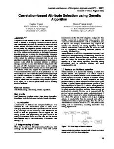
The refinery community has recognised the importance of the optimisation of production processes because of the benefits in terms of both profitability and environmental pollution. To this aim a huge number of variables need to be monitored by using adequate measuring devices. A possible alternative, which allows a remarkable reduction of monitoring and control costs, is to use VIs. Their core are mathematical models designed to estimate relevant variables, on the basis of available measured variables [7]. For the case of industrial plants, empirical models are usually designed exploiting both expert knowledge and experimental historical data [8], [9], [10], [11], [12]. In the proposed paper data from an SRU working in a large refinery in Sicily are used to design a VI, able to temporarily substitute the measuring devices, both in case of faults or programmed maintenance operations. Sulfur Recovery Unit (SRU) removes environmental pollutants from acid gas streams before they are released into the atmosphere. Acid gases are among the most dangerous air pollution factors and are one of the main causes of acid rain. The SRU consists of four identical sub-units, called sulfur lines, each capable to extract sulfur from acid gases produced by other processes in the refinery. A simplified scheme of Line 4 of the SRU is illustrated in Fig. 1 [13], [14]. The four sulfur lines work in parallel, taking two kinds of acid gases as input. The first kind, rich in H2S, called MEA gas, comes from the gas washing plants; the second, called SWS gas, rich in H2S and NH3 (ammonia), comes from the Sour Water Stripping (SWS) plant. Acid gases are burnt in reactors, where H2S is transformed into pure sulfur via a partial oxidation reaction with air. Gaseous combustion products coming from furnaces are cooled, causing the generation of liquid sulfur, which is collected in catch basins, then passed through high
temperature converters, where a further reaction leads to the formation of water vapor and sulfur. The remaining, unconverted gas (less than 5%), goes to a following plant for a final conversion phase.
models requires computing the autocorrelation function of the residuals and the correlation functions between the residuals and the model inputs [19]. When dealing with nonlinear systems, the analysis of residual properties is more cumbersome; however, a number of tests designed to detect whether the residual is unpredictable from all linear and nonlinear combinations of past inputs and outputs is reported in literature [6], [20], [21]. In practice, model validation requires that a number of normalized correlation functions between couples of sequences ψi and ψj are estimated. The sampled correlation function is: N −τ
φˆ
ψ iψ
j
Figure 1. Simplified scheme of Line 4 in the SRU plant
(τ ) =
∑ψ
i (t ) ψ j
N
(2)
∑ψ
2 i (t )
t =1
The final gas stream (tail gas) from the SRU contains residual H2S and SO2 which are measured by an on-line analyzer. Due to harsh working environment the analyzer is frequently off-line and during such periods it is neither possible to apply an automatic control policy (a manual control policy is anyway performed by plant operators) nor to monitor the plant products. A VI can be designed to solve such problems. In the proposed paper, the identification procedure applied for the modeling of the H2S concentration in the tail gas stream of Line 4 is described. Nevertheless, the described automatic procedure can be easily applied to other model identification problems. III.
THE MODEL ORDER SELECTION PROCEDURE
Several criteria have been proposed in the literature for the selection of the regressors of empirical models. Though there is a large number of works devoted to determine the proper model input structure for linear systems, there is relatively little work available in the field of nonlinear systems. A number of different approaches are based on deterministic suitability measures [1], False Nearest Neighbors (FNN) based algorithm [2], Lipschitz coefficients [3], [4] and Partial Least Squares regression (PLS) [4], to name just a few. Taking in mind that the VI is intended to replace measuring hardware during long time intervals, only NMA models, implemented via MLPs Neural Networks were considered [15], [16], [17], [18]. The general formulation for a NMA multi-input, single-output model is: [Y(k)]=f[IN1(k),…,IN1(k-n1),IN2(k),…,IN2(k-n2), …,INm(k),…,INm(k-nm)]
(1)
where Y(k) is the output sample at time k, INi (i= 1, 2, …, m) are the model input variables with their respective time delays ni, and f(·) is an unknown nonlinear function, usually approximated by using neural networks. In the case of SRU modeling five relevant inputs will be used, because of the expert suggestions, while regressors will be selected by using the proposed automatic procedure. In the theory of linear systems identification, a classical statistical approach to validate the identified linear
(t + τ )
t =1
N
∑ψ
2 j (t )
t =1
The following conditions need to be tested, for each input variable:
φ εε (τ ) = E [ε (t − τ )ε (τ )] = δ (τ )
(3)
φuε (τ ) = E [u (t − τ )ε (τ )] = 0 ∀τ
(4)
[
]
φ u 2 'ε (τ ) = E (u 2 (t − τ ) − u m2 (t )) ε (t ) = 0 ∀τ
[
]
(5)
φ u 2 'ε 2 (τ ) = E (u 2 (t − τ ) − u m2 (t ))ε 2 (t ) = 0 ∀τ
where E[·] is the mathematical expectation, ε(t) is the model residual, u(t) is the generic input variable, and the subscript m denotes the time average. The normalization adopted in (2) guarantees that introduced correlation functions are in the interval [-1, 1]. In practical applications, none of the reported correlation functions is exactly zero for any of the considered lags. Instead, it is checked that they lye within a suitable confidence band. The 95% confidence band is generally used corresponding to 1.96 / N , where N is the number of considered samples. The presence of values of the correlation functions lying significantly outside the confidence band for any time lag suggests that it is advisable to consider the corresponding lagged input in the model structure. The occurrence of this undesired behavior should anyway be critically analyzed taking into consideration any physical insight on the plant. The functions reported above have been used to develop an automatic design procedure which can be outlined as follows: 1) Select a starting model structure without regressors (any physical insight should be used at this point); 2) Design the corresponding neural model and compute its residual on a set of validation data;
3) Estimate correlation functions (3) ÷ (7); 4) Detect the variable and the lag corresponding to the largest peak outside the confidence band, for any of these functions; 5) Insert in the model regressor structure the regressor selected at Step 4) and go to Step 2). The procedure is repeated until all the correlation functions lye within the confidence band or no significant improvement is obtained. IV.
RESULTS
For the case of the SRU, data were collected and filtered with the help of plant technologists in order to represent the whole system dynamics. Moreover, a careful investigation of the available data was performed to detect either missing data or outliers. Each model was implemented by using MLP neural networks, trained with the Levenberg-Marquadt learning algorithm. A growing strategy has been used to select the number of hidden neurons on the basis of the model performance on a suitable validation data set. Experts have evidence that the process does not present any significant input-output
delay so that the starting model structure contains plant inputs at the current sampling time (IN(k)). In the following some significant steps of the evolution of the proposed procedure are described. After the best starting model was identified, the estimation of correlation functions was performed by using the validation data set. As an example of relevant results, the residual autocorrelation and the sets of the correlation functions, obtained for the first and the fifth inputs respectively are shown in Fig. 2. It can be observed that the model residual autocorrelation function lies significantly out of the corresponding confidence band. Moreover the analysis of φ u 5 ε ( τ ) suggests that more regressors are needed in the model for input #5. Graphs corresponding to remaining inputs looks like those reported for input #1 and they give evidence that no regressors are needed for these variables. The procedure therefore selected the regressor input IN5(k-10), corresponding to a relative extreme value in the correlation function.
φεε (τ ) Model error autocorrelation function
φuε (τ )
φu ε (τ )
φu
2'
2' 2
(τ )
φε (εu ) (τ )
2' 2
(τ )
φε (εu ) (τ )
ε
Input #1
φuε (τ )
φu ε (τ )
φu
2'
ε
Input #5 Figure 2. Correlation functions for the starting model structure
The procedure iterated a number of time leading to the model [Y(k)]=f[IN(k),IN5(k-10),IN5(k-2),IN5(k-1),IN5(k-3), (8) IN5(k-9),IN3(k-1),IN5(k-8),IN2(k-5),IN4(k-4)]
Where IN(k) is the model input vector of the starting model. The model has been implemented on refinery DCS to be tested on-line. The procedure stopped at this time, since all the correlation functions corresponding to model (8) lied inside the confidence band. The procedure described above showed to be adequate to solve the problem of regressor selection for the NMA model and can represent a valuable tool for people involved in VI design for industrial plants.
Tab. I, reported below, shows the improvements obtained at each step by using the proposed procedure. Underlined inputs represents the regressors that are added at each step. Tab. I gives also the number of hidden neurons for each MLP. The model performance are estimated by using the correlation coefficient between actual and estimated plant output, model error mean and standard deviation values. In Fig. 3 the trend of the correlation coefficient vs. the number of inputs is reported. In Fig. 4 and Fig. 5 the comparison between acquired data and corresponding estimations for two different lengths subset of H2S for the best model based on the proposed procedure are shown.
TABLE I. PERFORMANCE OF SUBOPTIMAL MODELS SUGGESTED BY THE PROPOSED PROCEDURE
Figure 4. Comparison of acquired data and corresponding estimations for a 65 test pattern subset of H2S for the best model based on the proposed procedure
Figure 5. Comparison of acquired data and corresponding estimations for a 1000 test pattern subset of H2S for the best model based on the proposed procedure
530
540
550
560 pattern
570
580
590
Figure 7. Comparison of acquired data and corresponding estimations for a 65 test pattern subset subset of H2S for the empirical model 0.5
The estimation capabilities of the best model are also analyzed in the following Fig. 6 where the 4-plot analysis, performed on the whole set on validation data, is shown.
Simulated H2S H2S 0.45
0.4
%
0.35
0.3
0.25
0.2
0.15 0
100
200
300
400
500 Test pattern
600
700
800
900
1000
Figure 8. Comparison of acquired data and corresponding estimations for a 1000 test pattern subset of H2S for the empirical model
Figure 6. 4-plot analysis for the best model based on the proposed procedure
V.
EMPIRICAL MODEL
In this section an empirical model of Line 4 is introduced for comparison purposes. Such a model was developed on the basis of suggestions given by plant experts and using a very conservative choice of models inputs; Also in this case, models have been implemented by using MLP neural networks trained with the Levenberg-Marquadt learning algorithm with the same sets of learning data. The estimation capabilities of the empirical model are analyzed in the following Fig. 7 and Fig. 8 where the comparison of acquired data and corresponding estimations for a subset of H2S validation data for the empirical model is shown. The performance are reported in Tab. 2
TABLE. 2. PERFORMANCE OF THE EMPIRICAL MODEL.
Correlation Coefficient Mean Error Standard Deviation
0.9111 -2.2246e-004 0.0130
In Fig. 9 the estimation capabilities of the empirical model, on the same set of validation data used in figure 6 are analyzed by the 4-plot analysis. Even if the performance obtained are comparable, the proposed procedure gave the best results. Moreover, the time spent in determining empirical model has been much more than that required by the automatic procedure proposed in this paper.
In this paper an automatic procedure is proposed to select model input structure in the design of a soft sensor. A SRU of a large refinery located in Sicily has been used as a case of study. The soft sensor has been designed to replace the on-line gas-chromatograph during maintenance in order to guarantee the continuity of the process monitoring and control. The approach is based on the evaluation of a set of cross-correlation functions between input variables and model residuals and it is used in the proposed paper to realize an automatic regressor selection algorithm for the design of nonlinear dynamic models. Taking into consideration that in the analyzed application the peaks of the output variable should be monitored with great accuracy, the proposed procedure allowed to improve performance obtained with an empirical model. Moreover the automatic procedure proposed has reduced the time spent in model design. REFERENCES [1] [2] [3]
[4] [5] [6] [7] [8] [9]
J.D. Bomberger and D.E. Seborg, Determination of model order for NARX models directly from input–output data, Journal of Process Control 8 (1998), 459–468. C. Rhodes and M. Morari, Determining the model order of nonlinear input/output systems, AIChE Journal 44 (1998), 151– 163. He, X. and Asada, H., A new method for identifying orders of input-output models for nonlinear dynamic systems. Proceedings of the ACC, San Francisco, CA, 1993, pp. 25202523. L. Fortuna, S. Graziani, G. Napoli, MG. Xibilia, “Comparing regressors selection methods for the Soft Sensor design of a Sulfur Recovery Unit”, proc. of MED06, Ancona, 2006. Feil, B.; Abonyi, J.; Szeifert, F. Model order selection of nonlinear input output models a clustering based approach. Journal of Process Control 2004, 14(6), 593–602. Billings SA, Voon WSF, (1991) Correlation based model validity tests for nonlinear models. International Journal Control 54:157–194. L. Fortuna, S. Graziani, A.Rizzo, MG. Xibilia, “Soft Sensors for Monitoring and Control of Industrial Processes”, Advances in Industrial Control, Springer, 2006. M.T. Tham, G.A. Montague, A.J. Morris and P. Lant, “SoftSensors for Process Estimation and Inferential Control”, Journal of Process Control, 1, 1991, 3-14. C. Bozzanca, S. Licitra, L. Fortuna and M.G. Xibilia, “Neural Networks for Benzene Percentage Monitoring in Distillation Columns”, Proc. of the Third Int. ICSC Symposia on Intelligent
[15] [16] [17] [18] [19] [20] [21]
Industrial Automation and Soft Computing, (ICSC Academic Press), Genova, Italy, 1999, 391-395. A. José de Assis, R. Maciel Filho, “Soft sensors development for on-line bioreactor state estimation”, Computers and Chemical Eng., 24, 2000, 1099-1103. S. Park, C. Han, “A non linear soft sensor based on multivariate smoothing procedure for quality estimation in distillation columns”, Computers & Chem. Eng., 24, 2000, 871-877. H.B. Su, L.T. Fan, J.R. Schlup, “Monitoring the process of curing of epoxy/graphite fiber composites with a recurrent neural network as a soft sensor”, Eng. Appl. Of Artificial Intelligence, 11, 1998, 293-306. L. Fortuna, A. Rizzo, M. Sinatra, M.G. Xibilia, “Soft analyser for a sulfur recovery unit”, Control Engineering Practice, Elsevier, vol 11, issue 12, Dec. 2003, pp. 1491-1500, Special issue Award winning applications- 2002 IFAC World Congress. L. Fortuna, S. Graziani, M.G. Xibilia, “Cross correlation analysis of residuals for the selection of the structure of Virtual Sensors in a refinery”, proc. ETFA05, Catania, Italy, Vol. 1, pp. 173-178,September 2005. J. Sjöberg et al., “Nonlinear Black-box Modeling in System Identification: a Unified Overview”, Automatica, Vol. 31, 12, pp. 1691-1724, 1995. A. Juditsky et al., “Nonlinear Black-box Modeling in System Identification: Mathematical Foundations”, Automatica, Vol. 31, 12, pp. 1725-1750, 1995. J. Sjöberg, H. Hjalmarsson, L. Ljung, “ Neural Networks in System Identification”, 10th IFAC Symp. On System Identificaton, Copenaghen, vol 2, pp. 49-72, 1994. L. Fortuna, S. Graziani, M.G. Xibilia, ”Virtual Instruments in refineries”, IEEE Instrumentation and Measurement Magazine, 8, 4, 26-34, Oct. 2005. T. Söderström and P. Stoica, System Identification. Englewood Cliffs,NJ: Prentice-Hall, 1989. Billings SA, Jamaluddin HB, Chen S, (1992) Properties of neural networks with applications to modelling non-linear dynamical system. International Journal Control 55:193–224 Mendes, E.M.A.M. and Billings, S.A. (2001) An alternative solution to the model structure selection problem. IEEE Transactions on Systems Man and Cybernetics Part A: Systems and Humans, 31 (6). pp. 597-608. ISSN 1083-4427.