Diss. ETH No. 16640
Selective Visualisation of Unsteady 3D Flow using Scale-Space and Feature-Based Techniques A dissertation submitted to the Swiss Federal Institute of Technology (ETH) Zürich for the degree of Doctor of Technical Sciences presented by Dirk Bauer Dipl.-Inf., University of Tübingen Swiss Federal Institute of Technology (ETH) Zürich born January 1, 1971 citizen of Germany accepted on the recommendation of Prof. Dr. Markus Gross, examiner Prof. Frits Post, co-examiner Dr. Ronald Peikert, co-examiner 2006
I
ABSTRACT During the recent years, visualisation has become an important part of scientific and engineering work. In parallel to the continuously increasing computing power available, the amount of data to be processed has become larger quickly. As is the case for the internet, there is a growing gap between the quantity of information that is theoretically available and the ability to efficiently process and handle this information. The extraction of the essential contents of the information and its reduction to a reasonable degree thus becomes a more and more important task. This also holds for the field of flow visualisation, where the underlying industrial datasets mostly are based on large computational grids originating from CFD (Computational Fluid Dynamics). A grid of this type often contains about one million or even more cells and nodes. The data given on these structures usually are vector and scalar fields, often given for several hundred time steps in the case of unsteady flow. As a consequence of this, the raw data consume significant disk space, and it is not possible to inspect and analyse every detail of the flow. Nevertheless there is a way out of this dilemma, since most of the flow details are not needed for understanding the general flow behaviour. The designers of water turbines, for example, are mainly interested in special flow structures like vortices, since these can cause undesired vibrations and resonance, leading to reduced efficiency, increased material abrasion, and in the worst case to machine damage. The essential parts of the flow, which are called features, can be extracted from the flow using special criteria and algorithms. The concept of feature extraction is part of the more general task of selective visualisation of flow. Several vortex criteria can be found in literature, which comprise the definition of line-type features like vortex core lines and surface-type features like vortex hulls. Also, a stream of mass-less particles in a flow can help identify its critical regions. All these paradigms can be applied to steady and time-dependent flow likewise. In the latter case, feature tracking is performed over successive datasets. In addition to conventional rendering and displaying techniques, virtual environments are becoming more and more popular in science and industry. VR technologies enhance the visual and acoustic perception by use of new input and output devices, such as lightsabers, 3D glasses, head trackers, large projection screens and stereo sound. They provide a way to “immerse” into a 3-dimensional graphical scene and thus to better explore and understand the structure of the visualised data. The field of flow visualisation can also benefit from these techniques and is therefore supported by VR development packages from several current visualisation platforms. The goal of this thesis is to investigate the essential features and behaviour of unsteady flow in the context of flow visualisation and industrial application. The focus is on new feature-based, region-based and integration-based methods for selective visualisation of 3D flow given in terms of vector and scalar fields on unstructured three-dimensional grids. Scale-space techniques known from computer vision improve the quality of the feature extraction. The results are also presented in a virtual reality environment and help our industry partners improve the design of turbomachinery parts, e.g. of water turbines.
II
ABSTRACT
III
ZUSAMMENFASSUNG In den letzten Jahren wurde Visualisierung zu einem wichtigen Bestandteil wissenschaftlichen und technischen Arbeitens. Parallel zur stetig wachsenden Rechnerleistung sind auch die zu verarbeitenden Datenmengen schnell angestiegen. Wie beim Internet existiert eine wachsende Lücke zwischen der Quantität an theoretisch verfügbarer Information und der Fähigkeit, diese noch effizient verarbeiten und mit ihr umgehen zu können. Das Herausfiltern wichtiger Inhalte aus der Information und deren Verringerung auf ein vernünftiges Mass wird deshalb zur immer wichtigeren Aufgabe. Dies trifft ebenfalls auf das Gebiet der Strömungsvisualisierung zu, wo die zugrundeliegenden industriellen Datensätze meist auf grossen, aus der rechnergestützten Strömungsdynamik stammenden Rechengittern basieren. Ein solches Gitter enthält oftmals etwa eine Million oder mehr Zellen und Knoten. Die auf diesen Strukturen gegebenen Daten sind gewöhnlich Vektor- und Skalarfelder, oft für mehrere hundert Zeitschritte im Falle einer zeitabhängigen Strömung. Als Folge davon verbrauchen die Rohdaten signifikanten Plattenplatz, und es ist nicht möglich, jedes Detail der Strömung zu betrachten. Trotzdem gibt es einen Ausweg aus diesem Dilemma, da die meisten Details für das Verständnis des generellen Strömungsverhaltens nicht benötigt werden. Die Designer von Wasserturbinen sind zum Beispiel hauptsächlich an speziellen Strukturen wie Wirbeln interessiert, da diese unerwünschte Vibrationen und Resonanz verursachen können, welche den Wirkungsgrad erniedrigen, das Material abnutzen und im schlimmsten Fall Maschinenschäden hervorrufen. Die wesentlichen Teile der Strömung, auch Merkmale genannt, können mittels spezieller Kriterien und Verfahren ermittelt werden. Die Merkmalsextraktion gehört zur selektiven Visualisierung. In der Literatur finden sich hierfür verschiedene Wirbelkriterien für Linien-Merkmale wie Wirbelkernlinien und Oberflächen-Merkmale wie Wirbelhüllen. Ein Partikelstrom kann ebenfalls helfen, die kritischen Regionen einer Strömung zu identifizieren. All diese Paradigmen können auf konstante und zeitabhängige Strömung gleichermassen angewendet werden. Im letzteren Fall wird Merkmalverfolgung auf aufeinanderfolgenden Datensätzen durchgeführt. Zusätzlich zu konventionellen Rendering- und Anzeigetechniken werden virtuelle Umgebungen in Wissenschaft und Industrie immer beliebter. VR-Technologien erweitern die visuelle und akustische Wahrnehmung durch Gebrauch neuer Peripheriegeräte, wie z.B. Laserschwerter, 3D-Brillen, Headtracker, grosse Projektionsflächen und Stereosound. Sie ermöglichen, in eine graphische 3D-Szene “einzutauchen“ und somit die Struktur der visualisierten Daten besser zu verstehen. Strömungsvisualisierung kann ebenfalls von diesen Techniken profitieren und wird deshalb durch VR-Entwicklungspakete mehrerer aktueller Visualisierungs-Plattformen unterstützt. Das Ziel dieser Dissertation ist, wesentliche Merkmale und Verhalten zeitabhängiger Strömungen im Kontext wissenschaftlicher Visualisierung und industrieller Anwendung zu untersuchen. Der Schwerpunkt liegt dabei auf merkmals-, gebiets- und integrationsbasierten Methoden zur selektiven Strömungsvisualisierung in Form von Vektor- und Skalarfeldern auf unstrukturierten 3D-Gittern. Aus der Computer Vision bekannte ScaleSpace-Techniken verbessern die Qualität der Merkmalsextraktion. Die Ergebnisse werden auch in einer VR-Umgebung präsentiert und helfen unseren Industriepartnern, das Design von Strömungsmaschinen, z.B. Wasserturbinen, zu verbessern.
IV
ZUSAMMENFASSUNG
V
ACKNOWLEDGEMENTS I especially want to thank my advisor Prof. Markus Gross and my co-advisor Dr. Ronald Peikert for their invaluable advise and guidance to this thesis. Their enthusiasm and comprehensive scientific and technical knowledge were always a great source of motivation and encouragement to me. It was a great time at the Computer Graphics Laboratory which led to new and inspiring insights and experiences, both professionally and personally. I’m also very grateful to all of the people at the ETH Zurich for providing such a convenient, friendly and stimulating environment. My thanks goes to Daniel Bielser, Milena Brendle, Oliver Bröker, Manuela Cavegn, Nurhan Cetin, Oscar Chinellato, Daniel Cotting, Prof. Walter Gander, Bruno Heidelberger, Prof. Hans Hinterberger, Andreas Hubeli, Richard Keiser, Nicky Kern, Oliver Knoll, Rolf Koch, Sathya Krishnarmurthy, Doo Young Kwon, Edouard Lamboray, Claudia Lorch, Reto Lütolf, Matthias Müller, Martin Näf, Prof. Kai Nagel, Christoph Niederberger, Mark Pauly, Brian Raney, Martin Roth, Samuel Hans Martin Roth, Prof. Bernt Schiele, Christian Sigg, Thomas Sprenger, Oliver Staadt, Matthias Teschner, Julia Vogel, Michael Waschbüsch, Tim Weyrich, Martin Wicke, Stephan Würmlin, Matthias Zwicker. In addition, I have to thank the employees from our industry partners VA Tech Hydro and Sulzer Hydro (the former Escher Wyss) for providing the industrial datasets which were used during this Ph.D. study. My special thanks goes to Mirjam Sick, Felix Muggli, Etienne Parkinson and Andreas Sebestyen for their friendly contact and advice. Special thanks goes to Daniela Hall, Mie Sato and Filip Sadlo for their support of some parts of the implementation and for many enjoyable and fruitful discussions on scale-space theory, vortex hulls, FrameMaker and other important issues. This work grew out of a long collaboration between the Computer Graphics Laboratory (CGL) of the ETH Zürich with our industry partners VA Tech Hydro (Zürich) and Sulzer Markets and Technology (Winterthur). The research project was funded by the Swiss Commission for Technology and Innovation (KTI) and by VA Tech/Sulzer under the project number 4917.1 KTS (October 2000 - September 2003).
VI
ACKNOWLEDGEMENTS
VII
CONTENTS 1 Introduction . . . . . . . . . . . . . . . . . . . . . . . . . . . . . . . . . . . . . . . . . . . . . . . . . . . . . . . 1 1.1
Flow Visualisation Pipeline . . . . . . . . . . . . . . . . . . . . . . . . . . . . . . . . . . . . . . . . 2 1.1.1 Data Input . . . . . . . . . . . . . . . . . . . . . . . . . . . . . . . . . . . . . . . . . . . . . . 2 1.1.2 Filtering . . . . . . . . . . . . . . . . . . . . . . . . . . . . . . . . . . . . . . . . . . . . . . . . 3 1.1.3 Mapping . . . . . . . . . . . . . . . . . . . . . . . . . . . . . . . . . . . . . . . . . . . . . . . 3 1.1.4 Rendering . . . . . . . . . . . . . . . . . . . . . . . . . . . . . . . . . . . . . . . . . . . . . . . 3
1.2
Motivation . . . . . . . . . . . . . . . . . . . . . . . . . . . . . . . . . . . . . . . . . . . . . . . . . . . . 3
1.3
Related Work . . . . . . . . . . . . . . . . . . . . . . . . . . . . . . . . . . . . . . . . . . . . . . . . . . 5
1.4
Contributions . . . . . . . . . . . . . . . . . . . . . . . . . . . . . . . . . . . . . . . . . . . . . . . . . . 6
1.5
Outline . . . . . . . . . . . . . . . . . . . . . . . . . . . . . . . . . . . . . . . . . . . . . . . . . . . . . . . 7
2 Basics of Flow Visualisation . . . . . . . . . . . . . . . . . . . . . . . . . . . . . . . . . . . . . . . . . . 9 2.1
Classification . . . . . . . . . . . . . . . . . . . . . . . . . . . . . . . . . . . . . . . . . . . . . . . . . . . 9 2.1.1 Application field . . . . . . . . . . . . . . . . . . . . . . . . . . . . . . . . . . . . . . . . . . 9 2.1.2 Gaining data for visualisation . . . . . . . . . . . . . . . . . . . . . . . . . . . . . . . 10 2.1.3 Level of data abstraction . . . . . . . . . . . . . . . . . . . . . . . . . . . . . . . . . . . 11 2.1.4 Spatial dimensionality of grid and data . . . . . . . . . . . . . . . . . . . . . . . . 12 2.1.5 Temporal dimensionality of data . . . . . . . . . . . . . . . . . . . . . . . . . . . . . 12
2.2
Cell and Grid Types . . . . . . . . . . . . . . . . . . . . . . . . . . . . . . . . . . . . . . . . . . . . 13
2.3
Data Fields . . . . . . . . . . . . . . . . . . . . . . . . . . . . . . . . . . . . . . . . . . . . . . . . . . . 16 2.3.1 Vector Fields . . . . . . . . . . . . . . . . . . . . . . . . . . . . . . . . . . . . . . . . . . . . 16 2.3.2 Scalar Fields . . . . . . . . . . . . . . . . . . . . . . . . . . . . . . . . . . . . . . . . . . . . 18
3 Flow Visualisation Techniques . . . . . . . . . . . . . . . . . . . . . . . . . . . . . . . . . . . . . . . 21 3.1
Direct Techniques . . . . . . . . . . . . . . . . . . . . . . . . . . . . . . . . . . . . . . . . . . . . . . 21 3.1.1 Arrow and Hedgehog Plots . . . . . . . . . . . . . . . . . . . . . . . . . . . . . . . . . 21
3.2
Integration-Based Techniques . . . . . . . . . . . . . . . . . . . . . . . . . . . . . . . . . . . . . 22 3.2.1 Streamlines and Particle Tracing . . . . . . . . . . . . . . . . . . . . . . . . . . . . . 22 3.2.2 Path Lines and Streaklines . . . . . . . . . . . . . . . . . . . . . . . . . . . . . . . . . . 24 3.2.3 Line Integral Convolution . . . . . . . . . . . . . . . . . . . . . . . . . . . . . . . . . . 24
3.3
Region-Based Techniques . . . . . . . . . . . . . . . . . . . . . . . . . . . . . . . . . . . . . . . . 26 3.3.1 Isosurfaces and Vortex Hulls . . . . . . . . . . . . . . . . . . . . . . . . . . . . . . . . 26
VIII
CONTENTS
3.4 Feature-Based Techniques . . . . . . . . . . . . . . . . . . . . . . . . . . . . . . . . . . . . . . . .28 3.4.1 Vector Field Topology and Critical Points . . . . . . . . . . . . . . . . . . . . . . .28 3.4.2 Vortex Core Lines and Parallel Vectors Operator . . . . . . . . . . . . . . . . . .30 3.4.3 Vortex detection method by Levy, Degani and Seginer . . . . . . . . . . . . .31 3.4.4 Vortex detection method by Sujudi and Haimes . . . . . . . . . . . . . . . . . .32 3.4.5 Vortex detection method by Banks and Singer . . . . . . . . . . . . . . . . . . .33 3.4.6 Vortex detection method by Miura and Kida . . . . . . . . . . . . . . . . . . . .34 3.4.7 Vortex detection method by Strawn, Kenwright and Ahmad . . . . . . . . .35 3.4.8 Mapping of vortex criteria to Parallel Vectors Operator . . . . . . . . . . . . .36 4 Scale-Space Techniques . . . . . . . . . . . . . . . . . . . . . . . . . . . . . . . . . . . . . . . . . . . .37 4.1 Multi-Resolution and Multi-Scale Representations . . . . . . . . . . . . . . . . . . . . . .38 4.1.1 Multi-resolution data representations . . . . . . . . . . . . . . . . . . . . . . . . . .39 4.1.2 Multi-scale data representations . . . . . . . . . . . . . . . . . . . . . . . . . . . . .40 4.2 Scale-Space Choice and Properties . . . . . . . . . . . . . . . . . . . . . . . . . . . . . . . . .41 4.3 Relation of Scale-Space to Fourier Theory . . . . . . . . . . . . . . . . . . . . . . . . . . . .43 4.4 Application to Image Processing and Computer Vision . . . . . . . . . . . . . . . . . . .45 4.5 Application to Flow Visualisation . . . . . . . . . . . . . . . . . . . . . . . . . . . . . . . . . . .47 4.6 Scale-Space Definition . . . . . . . . . . . . . . . . . . . . . . . . . . . . . . . . . . . . . . . . . . .48 4.7 Scale-Space Computation . . . . . . . . . . . . . . . . . . . . . . . . . . . . . . . . . . . . . . . .49 4.7.1 Structured Grids . . . . . . . . . . . . . . . . . . . . . . . . . . . . . . . . . . . . . . . . .49 4.7.2 Unstructured Grids . . . . . . . . . . . . . . . . . . . . . . . . . . . . . . . . . . . . . . .50 4.7.3 Computing Derivatives . . . . . . . . . . . . . . . . . . . . . . . . . . . . . . . . . . . .55 4.8 Results . . . . . . . . . . . . . . . . . . . . . . . . . . . . . . . . . . . . . . . . . . . . . . . . . . . . . . .56 5 Feature Extraction and Tracking . . . . . . . . . . . . . . . . . . . . . . . . . . . . . . . . . . . . . .57 5.1 Vortex Core Line Extraction . . . . . . . . . . . . . . . . . . . . . . . . . . . . . . . . . . . . . . .58 5.2 Extraction Of Vortex Cores in 3D . . . . . . . . . . . . . . . . . . . . . . . . . . . . . . . . . . .59 5.2.1 Computation of the connectivity structure for the unstructured grid . . .59 5.2.2 Setup of the two vector fields . . . . . . . . . . . . . . . . . . . . . . . . . . . . . . .60 5.2.3 Marking of the intersected edges . . . . . . . . . . . . . . . . . . . . . . . . . . . . .60 5.2.4 Finding the points of parallel vectors on all faces . . . . . . . . . . . . . . . . .60 5.2.5 Computation of the feature quality at a vertex . . . . . . . . . . . . . . . . . . .64 5.2.6 Filtering of the polylines . . . . . . . . . . . . . . . . . . . . . . . . . . . . . . . . . . .65 5.3 Feature Tracking in Time and Scale . . . . . . . . . . . . . . . . . . . . . . . . . . . . . . . . .65 5.3.1 Lifting principle and hypercubes . . . . . . . . . . . . . . . . . . . . . . . . . . . . .66 5.3.2 Structure of the lifted grid cells . . . . . . . . . . . . . . . . . . . . . . . . . . . . . .67 5.3.3 Construction of the feature mesh . . . . . . . . . . . . . . . . . . . . . . . . . . . . .68 5.3.4 Vortex tracking algorithm . . . . . . . . . . . . . . . . . . . . . . . . . . . . . . . . . . .70 5.4 Possible Extensions . . . . . . . . . . . . . . . . . . . . . . . . . . . . . . . . . . . . . . . . . . . . .72 5.4.1 Different cell types . . . . . . . . . . . . . . . . . . . . . . . . . . . . . . . . . . . . . . .72 5.4.2 Different feature definitions . . . . . . . . . . . . . . . . . . . . . . . . . . . . . . . . .73 5.4.3 Event detection . . . . . . . . . . . . . . . . . . . . . . . . . . . . . . . . . . . . . . . . . .73
IX
5.5
Results . . . . . . . . . . . . . . . . . . . . . . . . . . . . . . . . . . . . . . . . . . . . . . . . . . . . . . 76
6 Vortex Hulls . . . . . . . . . . . . . . . . . . . . . . . . . . . . . . . . . . . . . . . . . . . . . . . . . . . . . . 79 6.1
Basic Vortex Hull Algorithm . . . . . . . . . . . . . . . . . . . . . . . . . . . . . . . . . . . . . . 80
6.2
Enhanced Vortex Hull Algorithm . . . . . . . . . . . . . . . . . . . . . . . . . . . . . . . . . . . 82 6.2.1 Setup of the cross-section planes . . . . . . . . . . . . . . . . . . . . . . . . . . . . 83 6.2.2 Radial vortex hull expansion . . . . . . . . . . . . . . . . . . . . . . . . . . . . . . . . 84 6.2.3 Filtering of the ray lengths . . . . . . . . . . . . . . . . . . . . . . . . . . . . . . . . . . 86 6.2.4 Vortex hull assembly . . . . . . . . . . . . . . . . . . . . . . . . . . . . . . . . . . . . . . 87 6.2.5 Mesh postprocessing . . . . . . . . . . . . . . . . . . . . . . . . . . . . . . . . . . . . . 88
6.3
Results . . . . . . . . . . . . . . . . . . . . . . . . . . . . . . . . . . . . . . . . . . . . . . . . . . . . . . 89
7 Selective Particle Tracing . . . . . . . . . . . . . . . . . . . . . . . . . . . . . . . . . . . . . . . . . . . 95 7.1
Particle Tracing versus other Techniques . . . . . . . . . . . . . . . . . . . . . . . . . . . . . 96
7.2
Flow Regions of Interest . . . . . . . . . . . . . . . . . . . . . . . . . . . . . . . . . . . . . . . . . 96
7.3
Industrial Application . . . . . . . . . . . . . . . . . . . . . . . . . . . . . . . . . . . . . . . . . . . 98
7.4
Visualisation Techniques . . . . . . . . . . . . . . . . . . . . . . . . . . . . . . . . . . . . . . . . 100 7.4.1 Cell classification . . . . . . . . . . . . . . . . . . . . . . . . . . . . . . . . . . . . . . . 100 7.4.2 Particle seeding . . . . . . . . . . . . . . . . . . . . . . . . . . . . . . . . . . . . . . . . 101 7.4.3 Particle visibility . . . . . . . . . . . . . . . . . . . . . . . . . . . . . . . . . . . . . . . . 101 7.4.4 Particle tracing . . . . . . . . . . . . . . . . . . . . . . . . . . . . . . . . . . . . . . . . . 102 7.4.5 Conservation of mass . . . . . . . . . . . . . . . . . . . . . . . . . . . . . . . . . . . . 103 7.4.6 Particle rendering . . . . . . . . . . . . . . . . . . . . . . . . . . . . . . . . . . . . . . . 103
7.5
Results . . . . . . . . . . . . . . . . . . . . . . . . . . . . . . . . . . . . . . . . . . . . . . . . . . . . . 104
8 A Virtual Reality Application . . . . . . . . . . . . . . . . . . . . . . . . . . . . . . . . . . . . . . . . 107 8.1
Visualisation Systems and Virtual Environments . . . . . . . . . . . . . . . . . . . . . . . 108
8.2
The VR Application for Vortex Visualisation . . . . . . . . . . . . . . . . . . . . . . . . . . 111 8.2.1 System Overview . . . . . . . . . . . . . . . . . . . . . . . . . . . . . . . . . . . . . . . 111 8.2.2 The feature extraction module . . . . . . . . . . . . . . . . . . . . . . . . . . . . . 112 8.2.3 The COVER plugin . . . . . . . . . . . . . . . . . . . . . . . . . . . . . . . . . . . . . . 112 8.2.4 The feature processing module . . . . . . . . . . . . . . . . . . . . . . . . . . . . . 112
8.3
Results . . . . . . . . . . . . . . . . . . . . . . . . . . . . . . . . . . . . . . . . . . . . . . . . . . . . . 114
9 Conclusions . . . . . . . . . . . . . . . . . . . . . . . . . . . . . . . . . . . . . . . . . . . . . . . . . . . . . 117 9.1
Principal Contributions . . . . . . . . . . . . . . . . . . . . . . . . . . . . . . . . . . . . . . . . . 117
9.2
Discussion and Future Work . . . . . . . . . . . . . . . . . . . . . . . . . . . . . . . . . . . . . 118
A Colour Figures . . . . . . . . . . . . . . . . . . . . . . . . . . . . . . . . . . . . . . . . . . . . . . . . . . . 121 B References . . . . . . . . . . . . . . . . . . . . . . . . . . . . . . . . . . . . . . . . . . . . . . . . . . . . . . 125 C Implementational Aspects . . . . . . . . . . . . . . . . . . . . . . . . . . . . . . . . . . . . . . . . . 135 D Curriculum Vitae . . . . . . . . . . . . . . . . . . . . . . . . . . . . . . . . . . . . . . . . . . . . . . . . . 145
X
CONTENTS
XI
FIGURES Fig. 1.1 The flow visualisation pipeline with its four major phases . . . . . . . . . . . . . . . . . . 2 Fig. 2.1 Original and 1:10 scale test rig model of a Francis runner. . . . . . . . . . . . . . . . . 10 Fig. 2.2 The actual flow visualisation step in the visualisation pipeline . . . . . . . . . . . . . . 11 Fig. 2.3 Point cloud versus grid for the Stanford bunny model. . . . . . . . . . . . . . . . . . . . 13 Fig. 2.4 Different cell types used in visualisation grids . . . . . . . . . . . . . . . . . . . . . . . . . . 14 Fig. 2.5 Different grid types used in visualisation . . . . . . . . . . . . . . . . . . . . . . . . . . . . . . 15 Fig. 2.6 Definition of vortex strength in a plane perpendicular to the core line . . . . . . . 19 Fig. 3.1 Arrow plots (length proportional to velocity, constant length) . . . . . . . . . . . . . . 22 Fig. 3.2 Streamlines indicating a vortex at the stay vanes of a water turbine. . . . . . . . . . 23 Fig. 3.3 Stream surfaces indicating a vortex at the stay vanes of a water turbine. . . . . . . 24 Fig. 3.4 Line Integral Convolution image for guide and stay vanes of a water turbine. . . 25 Fig. 3.5 Lambda2 isosurfaces in a Francis turbine, connected components. . . . . . . . . . . 27 Fig. 3.6 Vorticity isosurface in a Francis turbine, false positives . . . . . . . . . . . . . . . . . . . 27 Fig. 3.7 Principle of the Levy method . . . . . . . . . . . . . . . . . . . . . . . . . . . . . . . . . . . . . . 31 Fig. 3.8 Principle of the Sujudi/Haimes method . . . . . . . . . . . . . . . . . . . . . . . . . . . . . . 32 Fig. 3.9 Principle of the Banks/Singer method . . . . . . . . . . . . . . . . . . . . . . . . . . . . . . . . 33 Fig. 3.10 Principle of the Miura/Kida method . . . . . . . . . . . . . . . . . . . . . . . . . . . . . . . . 34 Fig. 3.11 Principle of the Strawn/Kenwright/Ahmad method . . . . . . . . . . . . . . . . . . . . . 35 Fig. 4.1 The basic scale problem, as it occurs in the task of edge detection . . . . . . . . . . 38 Fig. 4.2 Multi-resolution representation of a two-dimensional image . . . . . . . . . . . . . . . 39 Fig. 4.3 Multi-scale representation of a two-dimensional image. . . . . . . . . . . . . . . . . . . 40 Fig. 4.4 Non-creation of local extrema (application to a 1-dimensional signal) . . . . . . . . 42 Fig. 4.5 Correspondance of sinc and rect function in spatial and frequency domain . . . 44 Fig. 4.6 Correspondance of Gaussian functions in spatial and frequency domain. . . . . . 44 Fig. 4.7 Feature extents in spatial and scale dimension . . . . . . . . . . . . . . . . . . . . . . . . . 46 Fig. 4.8 Gaussian smoothing and scale-space computation for images . . . . . . . . . . . . . . 46 Fig. 4.9 Hat functions as a simple example of finite elements . . . . . . . . . . . . . . . . . . . . 51 Fig. 4.10 Sharing of nodes by adjacent grid cells, indexing scheme . . . . . . . . . . . . . . . . 53 Fig. 5.1 How to find the solution points on all faces of the grid . . . . . . . . . . . . . . . . . . . 60 Fig. 5.2 Subdivision of a cell face and conversion of local coordinates. . . . . . . . . . . . . . 61 Fig. 5.3 Linear interpolation of the vector fields v and w on a triangle . . . . . . . . . . . . . 62 Fig. 5.4 Composing and orienting the line segments within a grid cell . . . . . . . . . . . . . . 64 Fig. 5.5 Definition of the feature quality of a vertex. . . . . . . . . . . . . . . . . . . . . . . . . . . . 64 Fig. 5.6 Filtering the polylines according to their vertex attributes . . . . . . . . . . . . . . . . . 65 Fig. 5.7 Example application of feature tracking in scale and time . . . . . . . . . . . . . . . . . 66 Fig. 5.8 The eight 3D boundary cubes of a 4D hypercube . . . . . . . . . . . . . . . . . . . . . . 67 Fig. 5.9 Construction of the 2D feature mesh from the 3D boundary cubes . . . . . . . . . 69 Fig. 5.10 The basic vortex tracking algorithm . . . . . . . . . . . . . . . . . . . . . . . . . . . . . . . . 70 Fig. 5.11 Filtering the triangle mesh by computing the feature quality . . . . . . . . . . . . . . 71 Fig. 5.12 Event detection using the feature mesh . . . . . . . . . . . . . . . . . . . . . . . . . . . . . 74 Fig. 5.13 Number of features at different scales. . . . . . . . . . . . . . . . . . . . . . . . . . . . . . . 76
XII
FIGURES
Fig. 5.14 Original draft tube dataset: geometry and instantaneous streamlines . . . . . . . .77 Fig. 5.15 Modernised draft tube: vortices are less articulate and harder to extract . . . . .77 Fig. 5.16 Vortex cores of modernised draft tube tracked through scales . . . . . . . . . . . . .77 Fig. 6.1 Principle of vortex hull construction . . . . . . . . . . . . . . . . . . . . . . . . . . . . . . . . .80 Fig. 6.2 The original vortex hull construction algorithm (fixed sampling intervals) . . . . . .81 Fig. 6.3 Vortex core line and computed vortex hull . . . . . . . . . . . . . . . . . . . . . . . . . . . .81 Fig. 6.4 Location of the cross-section planes in the middle of the core line segments . . .82 Fig. 6.5 Plane coordinate system for the rays, and definition of its basis vectors . . . . . . .83 Fig. 6.6 Vortex hull cross-sections based on different scalar fields. . . . . . . . . . . . . . . . . .84 Fig. 6.7 Ray traversal through the cells of the unstructured grid . . . . . . . . . . . . . . . . . . .85 Fig. 6.8 High frequencies of the ray lengths in the cross-sections of a vortex hull . . . . . .86 Fig. 6.9 Smoothing the ray lengths by use of a filter mask. . . . . . . . . . . . . . . . . . . . . . . .86 Fig. 6.10 Construction of the final vortex hull from the ray endpoints . . . . . . . . . . . . . .87 Fig. 6.11 Storage of mesh vertices and application of umbrella operator . . . . . . . . . . . .89 Fig. 6.12 Vortex core line and hull construction for the bent helix dataset . . . . . . . . . . .91 Fig. 6.13 Vortex hulls based on Levy method and distance field. . . . . . . . . . . . . . . . . . .91 Fig. 6.14 Vortex hulls. High-frequency noise requires smoothing . . . . . . . . . . . . . . . . . .92 Fig. 6.15 Vortex hulls. Median ray filtering reduced noise . . . . . . . . . . . . . . . . . . . . . . .92 Fig. 6.16 Vortex hulls. Laplacian mesh fairing without ray filtering . . . . . . . . . . . . . . . . .93 Fig. 6.17 Vortex hulls. Median ray filtering and subsequent Laplacian mesh fairing . . . .93 Fig. 7.1 ROI definition by a scalar field and threshold . . . . . . . . . . . . . . . . . . . . . . . . . .97 Fig. 7.2 Photograph of a cavitating vortex rope on the test rig . . . . . . . . . . . . . . . . . . . .98 Fig. 7.3 Variations of relative pressure at the runner blades of a Francis turbine . . . . . . .99 Fig. 7.4 Variations of relative pressure in the draft tube of a Francis turbine . . . . . . . . . .99 Fig. 7.5 Classification of cells, particle visibility, and tiles of quasi-random points . . . . .100 Fig. 7.6 Pseudo-random samples, jittered regular samples, Sobol’ points, tiles . . . . . . .101 Fig. 7.7 Smooth visibility transition by two scalar thresholds. . . . . . . . . . . . . . . . . . . . .101 Fig. 7.8 Pseudo-code of the selective particle tracer. . . . . . . . . . . . . . . . . . . . . . . . . . .102 Fig. 7.9 Clamping local coordinates at the grid boundary. . . . . . . . . . . . . . . . . . . . . . .103 Fig. 7.10 Cavitation bubbles near Kaplan runner blades, rendered as spheres . . . . . . .104 Fig. 7.11 Particle stream through a storage pump, rendered as spheres . . . . . . . . . . . .105 Fig. 7.12 Vortex rope in Francis draft tube, rendered as streamlets. . . . . . . . . . . . . . . .105 Fig. 8.1 A typical COVISE network . . . . . . . . . . . . . . . . . . . . . . . . . . . . . . . . . . . . . . .108 Fig. 8.2 The Inventor-based COVISE standard renderer . . . . . . . . . . . . . . . . . . . . . . . .109 Fig. 8.3 Typical VR environments . . . . . . . . . . . . . . . . . . . . . . . . . . . . . . . . . . . . . . . .109 Fig. 8.4 A graphical scene and the standard main menu of the COVER renderer . . . . .110 Fig. 8.5 System architecture for the VR vortex visualisation framework. . . . . . . . . . . . .111 Fig. 8.6 A typical scene showing COVER and VR application menus and vortex hulls. .113 Fig. 8.7 Vortex core lines and hulls of the original draft tube design . . . . . . . . . . . . . . .115 Fig. 8.8 Vortex core lines and hulls of the modified draft tube design. . . . . . . . . . . . . .115
XIII
Fig. A.1 Vortex extraction for a Francis turbine . . . . . . . . . . . . . . . . . . . . . . . . . . . . . . 121 Fig. A.2 Vortex tracking in scale and time . . . . . . . . . . . . . . . . . . . . . . . . . . . . . . . . . . 122 Fig. A.3 Vortex hulls and VR application . . . . . . . . . . . . . . . . . . . . . . . . . . . . . . . . . . . 123 Fig. A.4 Industrial motivation and selective particle tracing . . . . . . . . . . . . . . . . . . . . . 124 Fig. C.1 The enhanced vortex hull construction algorithm . . . . . . . . . . . . . . . . . . . . . . 136 Fig. C.2 The algorithm for finding the endpoint of a ray . . . . . . . . . . . . . . . . . . . . . . . 137 Fig. C.3 Mapping of a quadrangle between computational and physical space . . . . . . 138 Fig. C.4 The algorithm for intersecting a ray with a quadrangle cell face . . . . . . . . . . . 141 Fig. C.5 Different intersection situations . . . . . . . . . . . . . . . . . . . . . . . . . . . . . . . . . . . 142 Fig. C.6 Further intersection situations . . . . . . . . . . . . . . . . . . . . . . . . . . . . . . . . . . . . 143 Fig. C.7 The modified function FindEndpointOfRay() . . . . . . . . . . . . . . . . . . . . . . . . . . 144
XIV
FIGURES
XV
TABLES Table 3.1 Different cases of velocity gradient eigenanalysis and vector field topology . . 29 Table 3.2 Different vortex criteria and their parallel vectors representation . . . . . . . . . . 36 Table 4.1 Performance analysis of scale-space computation . . . . . . . . . . . . . . . . . . . . . 56 Table 5.1 Properties of different cell types and extension from 3 to 4 dimensions . . . . . 72 Table 5.2 Mapping of triangle intersection types to event types. . . . . . . . . . . . . . . . . . . 75 Table 6.1 Performance analysis of the vortex hull computation . . . . . . . . . . . . . . . . . . . 90 Table 8.1 Performance analysis of the VR application for vortices . . . . . . . . . . . . . . . . 114
XVI
TABLES
C H A P T E R
1
1
INTRODUCTION
During the recent years, visualisation on digital computers has become an important part of scientific and engineering work, especially in application fields like medicine, the natural sciences, automotive and aircraft industry. In parallel to the continuously increasing computing power available, the amount of data to be processed has grown rapidly. As in the case of the internet, there is a growing gap between the quantity of information that is theoretically available and the ability to efficiently process and handle this information. The extraction of the essential contents of the information and its reduction to a reasonable degree thus becomes a more and more important task. This also holds for the field of flow visualisation, where the underlying industrial datasets mostly are based on large computational grids originating from CFD simulations (Computational Fluid Dynamics). A grid of this type often contains millions of cells and nodes. The data stored on these structures usually are vector and scalar fields, often given for several hundred time steps in the case of unsteady flow. As a consequence of this, the raw data consume significant disk space, and it is for a human being not possible to inspect and analyse every detail of the flow. Nevertheless there is a way out of this dilemma, since most of the flow details are not needed for understanding the general flow behaviour. The designers of industrial water turbines, for example, are mainly interested in special flow structures like vortices since these can cause undesired vibrations and resonance, which lead to reduced efficiency, enhanced material abrasion, and in the worst case to machine damage. The essential parts of the flow, which are called features, can be extracted from the flow data using special criteria and algorithms. This dissertation investigates the essential features and behaviour of unsteady flow in the context of scientific visualisation and industrial application. The focus is on new feature-, region- and integration-based methods for selective visualisation of flow given in terms of vector and scalar fields on unstructured three-dimensional grids. The thesis also treats the fairly new idea to apply scale-space techniques to the field of flow visualisation. 1
2
1
INTRODUCTION
Originally proposed in the context of image processing, scale-space techniques have been used for structured grids in the field of computer vision. However, their potential for flow visualisation was previously not exploited, maybe due to the major changes in implementation required for the unstructured grids mainly used in this field. The goal of this thesis is to benefit from scale-space methods to improve the quality of feature extraction and tracking, which is performed in terms of vortex core line detection. Additionally, vortex hulls for unstructured grids are presented to enhance the visual perception of vortex sizes and shapes. Furthermore, a modified particle tracer is proposed which allows for concentrating on selected regions-of-interest (ROIs), thereby reducing occlusion problems, visual artifacts and storage requirements. Some of the results are also presented in a virtual reality environment and help our industry partners improve the design of turbomachinery parts, e.g. of water turbines. The remainder of this chapter is structured as follows: Section 1.1 sets the context of this thesis by describing the flow visualisation process. Section 1.2 motivates the approaches presented in this thesis, whereas Section 1.3 shortly discusses some related work done in this area before. Our major contributions to the field are listed in Section 1.4, and Section 1.5 concludes this chapter with an outline of the dissertation.
1.1
FLOW VISUALISATION PIPELINE The overall visualisation process can be seen as a pipeline consisting of four major phases: data input, filtering, mapping, rendering [HM90]. Figure 1.1 illustrates the process from gaining scientific flow data until rendering of the graphical results on a computer display. The following sections will discuss the individual stages of the pipeline in more detail.
data input
flow measurements flow simulation (CFD)
FIGURE 1.1
1.1.1
filtering
deriving data fields data smoothing
mapping
feature extraction particle tracing
rendering
visualisation platforms VR environments
The flow visualisation pipeline with its four major phases.
Data Input There are two basically different sources for the input data of the visualisation process, a physical and a virtual one. The first is to really establish a physical flow by constructing real-world models (e.g. a turbo-machine in a wind channel) and to measure its characteristic data (such as velocity and pressure), using sensors mounted at the test object (such as wing tips of an airplane or the draft tube of a water turbine). The alternative way is to do Computational Fluid Dynamics (CFD), i.e. to numerically simulate the flow on a digital computer by solving Navier-Stokes equations. In both cases, the results are produced for a predefined grid in the computational domain and stored as datasets on disk.
1.2
1.1.2
MOTIVATION
3
Filtering The filtering step is in a sense the preprocessing of the actual visualisation (whereas from the CFD viewpoint, the visualisation step is often called CFD postprocessing, see [Bun89]). Filters convert a CFD dataset to another one by modifying its contents. Typical examples are: calculating derived fields from the input data fields (e.g. vorticity from velocity), building 2D slices from 3D data, or smoothing the input data using Gaussian filters.
1.1.3
Mapping Mapping is the central part of the visualisation process. Its task is to produce geometrical primitives (e.g. points, lines or triangle meshes) which depict the essential information of the flow data. Typical examples are the computation of isosurfaces and contour plots from scalar fields, as well as feature extraction and particle tracing. Often the result data must be postprocessed (e.g. by computing connected components of triangle meshes).
1.1.4
Rendering The rendering phase concludes the visualisation process by converting the 3D geometric primitives to a 2D image consisting of coloured pixels. Common visualisation platforms such as AVS 5, AVS Express or Covise offer sophisticated renderers for a variety of purposes, e.g. the Covise system includes a conventional renderer as well as a special renderer supporting virtual environments (see Chapter 8).
1.2
MOTIVATION This dissertation mostly deals with the filtering stage and mapping stage of the flow visualisation pipeline. It particularly focuses on methods for selective visualisation of flow features like vortices, vortex hulls and particle movements in time-dependent CFD data given on unstructured three-dimensional grids. As mentioned above, automatic extraction of features is a promising strategy to cope with the large amount of data produced by such time-dependent CFD simulations. The computational time for this type of simulation is typically in the order of days, which justifies the time spent on postprocessing the data by extracting features in a batch run. In fact, automatic feature extraction can achieve substantial data reductions while still permitting the visualisation of the essential parts of the flow. It can be used for visually browsing the results or in conjunction with other visualisation methods. However, the implementation of this strategy leads to the following problems: 1. Many flow features are of fractal nature, that means that there is no unique definition of their feature size. Depending on the observation scale, different sets of features can be observed. Usually, the scale is implicitly defined when an extraction method is designed. Instead, it would be preferable to let the user specify the scale interactively while viewing the result data. 2. Most methods require numerical computation of spatial derivatives, which is known to cause a roughening of the data. Smoothing the data can reduce this effect, but it is not trivial to find an appropriate smoothing kernel when dealing with irregular grids and highly varying cell sizes, as often occur in CFD datasets.
4
1
INTRODUCTION
3. When features are extracted from time-dependent data, animating them can cause popping effects with features suddenly appearing or disappearing. These artifacts can be alleviated by incorporating temporal in addition to spatial smoothing. As we will see in Chapter 4, scale-space techniques can successfully be applied to the field of computer vision, where feature extraction has already been practised for a long time. These techniques smooth the input data using Gaussian kernels, the standard deviation σ of which can be any positive real number. The hereby defined scale axis plus the spatial axes span the scale-space. Features thus not only have spatial extents but also a certain scale extent. They can therefore be searched and found in scale-space. This technique has the potential to solve the problems mentioned above also for the flow visualisation field. The idea is now to combine scale-space methods with feature extraction in order to track features along time or, alternatively, along scale. Whereas the first scenario is obvious, the second one should help identify fragmented features while still keeping their positional accuracy. Furthermore, the quality of the results should be improved, because estimating derivatives of the flow fields needs no extra filtering due to the presmoothed data at higher scale levels. Furthermore, subsetting of the resulting vortex core lines should be automated and need fewer heuristic parameters than in previous implementations (see Chapter 5). The concept of feature extraction is part of the more general task of selective visualisation of flow. A variety of vortex detection criteria can be found in literature, which comprise the definition of line-type features like vortex core lines and surface-type features like vortex hulls. Also, a stream of mass-less particles in a flow can help identify its regions-ofinterest. All these paradigms can be applied to steady and time-dependent flow likewise. Besides the feature tracking system discussed above, we want to design a method for adding vortex hulls to the extracted vortex core lines, which in contrast to other approaches is capable to operate on unstructured grids (see Chapter 6). The idea is to combine the advantages of line-type features (clear separability of different vortices) with those of region-type features (better notion of vortex shape and size). The new method should permit the choice of different scalar fields and thresholds to define the boundary of the vortex, as well as filtering and fairing operations to smooth the resulting tubes. Furthermore, we want a modified particle tracer which reduces the number of particles to be processed by concentrating on certain regions-of-interest (see Chapter 7). A cell classification scheme and a special particle seeding scheme will help keeping the particle density constant, while blending operations will allow smooth transitions at the boundaries. In addition to conventional rendering and displaying techniques, virtual environments are becoming more and more popular in science and industry. VR technologies enhance the visual and acoustic perception by use of new input and output devices, such as laser swords, 3D glasses, head trackers, large projection screens and stereo sound. They provide a way to “immerse” into a 3-dimensional graphical scene and thus to better explore and understand the structure of the visualised data. The field of visualisation can also benefit from these techniques and is therefore supported by VR development packages from current visualisation platforms. We will in Chapter 8 present a framework which allows to interactively explore results from our visualisation methods in such a virtual environment. Since the filtering and mapping stage of the flow visualisation pipeline takes significant time, the approach is to store the results to disk and transferring them to the VR system, which can render and display them at comfortable frame rates.
1.3
1.3
RELATED WORK
5
RELATED WORK This section summarises some important work which was done in the context of flow visualisation prior to this dissertation. More detailed descriptions of the referred papers will be given in the appropriate chapters later in this thesis. The general field of visualisation was first defined in 1987 by McCormick, DeFanti and Brown in their groundbreaking NFS report [MDB87], which stated the necessity of and showed the direction for further research. The vast application field of flow visualisation was described in detail in 1989 by Buning [Bun89] and later by Post, Laramee et al. in several articles [HPvW94, PvW94, PVH+03, LHD+04]. Multi-scale and multi-resolution data representations had already been used during the 1970s [Kli71], but without solving the problem of relating features of different scales to each other. The foundations of the scale-space theory were then established in the 1980s by Witkin [Wit83, WT83] and Koenderink [Koe84]. Originally restricted to image processing and vision, the theory was in the 1990s extended by Florack, Romeny et al. [FtHRKV92] and Lindeberg [Lin94], who gave a thorough compendium of scale-space theory and application fields at that time. Nonlinear scale-spaces based on anisotropic diffusion were used by Perona and Malik [PM87] for edge detection and by Diewald et al. [DPR00] for visual exploration of vector fields. Our goals are, beyond visual exploration, to algorithmically extract features as geometric objects and to improve this process by exploiting the multi-scale nature of the features. For this purpose, we will use isotropic linear scale-spaces, since they better fit to our requirements. Luerig, Westermann et al. [LGE97, WE97] performed feature extraction from volumetric data in scale-spaces based on wavelets. However, to keep the spatial resolution also at higher scale levels, we will not construct a multi-resolution pyramid. Also, such a pyramid would yield a too coarse sampling along the scale axis. For the purpose of feature tracking, it is preferable to have no prescribed sampling. Different vortex detection methods were proposed by Levy et al. [LDS90], Sujudi/ Haimes [SH95b, SH95c], Banks/Singer [BS94, SB94], Miura/Kida [MK96], and Strawn/Kenwright/Ahmad [SKA98, SKA99]. Based upon their line-type definitions of a vortex, Roth and Peikert [RP99, Rot00] proposed the parallel vectors operator, a more general scheme which all of the above vortex criteria can be embedded in by formulating them in terms of two vector fields. However, all these approaches only solve the problem for steady flow fields in 3D. Our goal is to also track vortices over time or scale using a 4D extension (published in [BP02b]) of the parallel vectors algorithm. Feature tracking was performed e.g. by Silver et al. [SZF+91, SW96] and Reinders et al. [RPS99, Rei01]. Most of the existing tracking methods operate on features extracted from 3D grid cells in single datasets. In contrast, our approach is to extend the grid cells by one dimension and to extract the features from these lifted cells, which are in our case 4D hypercubes. This reflects the same lifting principle as the Marching Cube algorithm uses for isosurface extraction in 3D, a problem which was originally regarded as tracking 2D contour plots along the z axis of the 3D grid. An advantage of our feature tracking method is that it needs no heuristics like spatial overlap [SW96] or shape attributes [RPS99], while it can still handle features moving by more than one grid cell per dataset.
6
1
INTRODUCTION
Vortex hulls have been treated by Zabusky [ZBP+91], Banks and Singer [BS94], Sadarjoen [Sad99], Roth [Rot00] and recently by Garth et al. [GTS+04]. Most approaches regard the vortex hull as a deformable model (see Terzopoulos and Fleischer [TF88]) which has a centerline and is extended until a certain condition is met, for instance when the pressure becomes too large. However, many implementations are based on rectilinear or structured grids. We will also stick to the deformable model principle but develop a method working on unstructured grids and for termination criteria based on different scalar fields. Our extension principle is more sophisticated than the one previously presented in [BP02a] and therefore needs less computational time. Particle tracing is actually a well-known standard technique (see the description by Sadarjoen et al. [SvWHP97]). Nevertheless, it is hard to find better techniques for timedependent vector fields. One of the key problems is to maintain the particle density over time. For streamline integration, streamline placement techniques were introduced by Turk and Banks [TB96]. Our approach [BP02a] takes advantage of the mass conservation property of physical flow fields and uses a quasi-random particle seeding scheme (see [SH95, SMA00]) in conjunction with a buffer cell mechanism. The restriction to a certain region-of-interest surrounded by a ring of buffer cells saves significant computational effort. Based upon two scalar thresholds, a smooth blending of particles entering and leaving the ROI is achieved. For our VR application, we chose the Covise visualisation platform developed at the University of Stuttgart [HLR04] and now being distributed by the spin-off company VisEnSo [VIS04]. The VR renderer contained in this package can be enhanced by userprogrammed plugins [VIS03], which enabled us to transfer our visualisation results into a virtual environment for interactive exploration and enhanced visual perception.
1.4
CONTRIBUTIONS The goal of this thesis is to investigate the essential features and behaviour of unsteady flow in the context of flow visualisation and industrial applications. The focus is on new feature-based, region-based and integration-based methods for selective visualisation of 3D flow given in terms of vector and scalar fields on unstructured three-dimensional grids. Scale-space techniques known from computer vision improve the quality of the feature extraction. The results are also presented in a virtual reality environment and help our industry partners improve the design of turbomachinery parts, e.g. of water turbines. The main contributions of this thesis are: •
an application of scale-space techniques to the field of flow visualisation,
•
a computational scheme for constructing the scale-space on unstructured CFD grids,
•
an algorithm for extracting and tracking vortex core lines over time and scale,
•
a scalar-field based method for constructing vortex hulls around core lines,
•
a particle tracer for selective visualisation of regions-of-interest in flow fields,
•
a framework for interactive visualisation of flow features in virtual reality.
1.5
1.5
OUTLINE
7
OUTLINE The remaining chapters of this thesis are organised as follows: •
Chapter 2 gives a brief overview on the fundamentals of visualisation in general and of flow visualisation in particular. After a presentation of several different ways to categorise visualisation, the most important grid and data types used in flow visualisation are discussed. The definitions given here are fundamental for the flow visualisation techniques described in the following chapters.
•
Chapter 3 gives a short overview on several basic techniques for flow visualisation, most of which were used as ingredients for the algorithms and methods presented in the later chapters of the thesis. A few representatives of the flow visualisation categories mentioned in the previous chapter are discussed, namely of the direct, integrationbased, region- and feature-based flow visualisation techniques.
•
Chapter 4 gives an overview of some important data representations dealing with different levels of resolution or scale. It presents the scale-space representation and its special properties, along with some application examples from image processing and computer vision. The use of scale-space methods for flow visualisation is also motivated. At the end of the chapter, several methods for computing the scale-space representation on different grid types are discussed and compared, and a newly developed method for computing the scale-space on unstructured grids is presented.
•
Chapter 5 recapitulates the parallel vectors operator, a general vortex core line extraction algorithm introduced by Roth and Peikert [RP99], and describes the adaptations and simplifications to be made in the context of a scale-space analysis. It is then shown how a 4D extension of this algorithm is able to track vortices in either the temporal or in the scale domain. Finally, both numerical and visual results are given.
•
Chapter 6 presents an implementation of vortex hulls for vortex core lines on unstructured grids, which allows to select from different hull shapes and scalar fields, to define suitable thresholds, and to smooth the surfaces of the constructed tubes. The combination of line-type features (vortex core lines) and region-type features (vortex hulls) leads to plastic illustrations of vortex extents and still clearly separable features.
•
Chapter 7 explores techniques for visualising selected flow structures in time-dependent data by use of a modified, sophisticated particle tracer. A particle seeding scheme based on quasi-random numbers is proposed, which minimises visual artifacts such as clusters or patterns. By constraining the visualisation to a region of interest, occlusion problems are reduced and storage efficiency is gained. The primary industrial application is the visualisation of the vortex rope, a rotating helical structure which builds up in the draft tube of a water turbine. In two related applications, the cavitation regions near the runner blades of a Kaplan turbine and a water pump are visualised.
•
Chapter 8 presents a framework for transferring results of the vortex core extraction and vortex hull construction to a virtual environment. A file system based approach is used to decouple the rendering phase from the computationally expensive data acquisition and feature extraction procedures. As a consequence of this, the VR application is able to efficiently load and handle the vortex result data. The user can thus navigate through the result datasets at comfortable frame rates and interactively select, mark and remove vortex structures from the screen.
8
1
INTRODUCTION
•
Chapter 9 concludes the dissertation with a summary of the main contributions, a discussion of advantages and drawbacks of the presented approaches, and some ideas for future research.
•
Appendix A contains coloured versions of some result images shown in the previous chapters, especially concerning feature extraction and tracking, vortex hulls, the VR application, and selective particle tracing.
•
Appendix B contains all literature references of this thesis.
•
Appendix C contains some more detailed explanations on how the vortex hulls of Chapter 6 were constructed. The focus is on the problem of intersecting a given ray with a quadrangle face of a hexahedral cell in 3D space, which can be planar or nonplanar. Due to the discrete nature of the underlying unstructured grids and due to noise contained in some of the raw industrial datasets we investigated, a number of nontrivial numerical problems had to be solved in addition to the theoretical procedure.
•
Appendix D contains a curriculum vitae of the author of this thesis.
C H A P T E R
2
2
BASICS OF FLOW VISUALISATION
Flow visualisation has been an important and interesting part of visualisation for decades. In this chapter, we give a brief overview on the fundamentals of visualisation in general and of flow visualisation in particular. After presenting several different ways to categorise visualisation, we will discuss the most important grid and data types used in flow visualisation. The definitions given here are fundamental for the flow visualisation techniques described in the following chapters.
2.1
CLASSIFICATION Although visualisation has a long history, its meaning for scientific work was not fully recognised until the late 1980s. In their pioneering NSF report on visualisation in scientific computing [MDB87], McCormick, DeFanti and Brown gave a general definition of the subject and pointed out the need and direction for further research. Since the general field of visualisation, as well as that of flow visualisation, offers a wide range of methods and applications, no trivial or even canonical classification of the subject exists [HPvW94]. Also, the special conditions of any application field have a strong influence on the suitability of each visualisation method, and thus on the preferred choice. In this section, we will present several possible criteria for a categorisation of visualisation.
2.1.1
Application field The perhaps most intuitive criterion is the application field where data are to be visualised. A coarse differentiation can be made between information visualisation and scientific visualisaton. The first one mostly deals with discrete and higher-dimensional data, which is often stored in tables or relational databases and does not have a well-defined metrics. Typical methods of information visualisation include chart diagrams, parallel coordinates, scatter plots and perspective walls. A wide selection of business applications are available which cover the most important needs of this area. 9
10
2
BASICS OF FLOW VISUALISATION
This thesis concentrates on the other type, scientific visualisation, and one of its most common subareas, flow visualisation. Typical applications of flow visualisation can be found in (but are not restricted to) aerodynamics, automotive industry, geology, medicine, meteorology, and turbomachinery design. 2.1.2
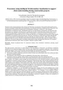
Gaining data for visualisation In this chapter, we use the term “flow visualisation” for what is actually computational flow visualisation. This means that the datasets to be visualised were created by numerical simulations based on physical models, e.g. using the Navier-Stokes equations. The simulated flow data (especially the velocity and pressure data) are stored in datasets and serve as a basis for various computational methods to visualise the flow. In this thesis, we will mainly refer to this type of gaining and processing the information contained in a flow. However, it should be kept in mind that flow visualisation can also be done the “good old way” using flow experiments and empiricism. One example is the use of test rigs for reduced scale models of existing turbines, as is done by our industry partner VA Tech Hydro, the former Escher Wyss (a size comparison of test model and real counterpart of a Francis runner is shown in Figure 2.1). The flow behaviour within these models can for instance be observed and recorded using high-speed cameras and stroboscope lighting. Another possibility is to inject dye into a flow and to photographically record the movement and distribution of the coloured water particles. .
FIGURE 2.1
Original and 1:10 scale test rig model of a Francis runner (image courtesy of VA Tech Hydro, Zurich). See also Colour Figure A.1 on page 121.
Although numerical simulation and computational visualisation give better insight into the flow behaviour and help reduce the developing costs of technical devices (such as machine parts of a water turbine), experimental and empirical flow visualisation are still indispensable for proving the theoretically computed results. For cost reasons, such flow
2.1
CLASSIFICATION
11
experiments are only performed for turbomachinery designs which have in advance been optimised using computational visualisation methods. 2.1.3
Level of data abstraction Visualisation methods can also be categorised according to the effort they require in comparison to other steps of the visualisation pipeline. Post, Laramee et al. distinguish between three fundamentally different types of visualisation methods, namely direct, integrationbased, and feature-based visualisation methods [PVH+03, LHD+04]. Generally, it can be stated that the computational complexity of a method rises with its level of data abstraction (see Figure 2.2). On the other hand, a more sophisticated visualisation method leads to more physically meaningful results, which reduces the amount of data to proceed with.
data acquisition
data acquisition
data acquisition
direct visualisation using simple glyphs
flow integration point location data evaluation
data derivation grid preprocessing feature extraction result filtering
rendering
rendering rendering
direct visualisation
FIGURE 2.2
integration-based visualisation
feature-based visualisation
The actual flow visualisation step in the visualisation pipeline.
In the simplest case, the user is interested in a quick, intuitive, and direct visualisation of the data. This can often be achieved by relatively fast and simple methods, e.g. the velocity data of a flow can easily be drawn as an arrow plot if the flow is 2-dimensional (for 3 dimensions, the case is more difficult to handle due to perception and occlusion problems). A similar method is the use of hedgehog plots as suggested by Klassen and Harrington [KH91] and implemented in The Visualisation Toolkit (VTK) by Schroeder, Martin and Lorensen [SML03]. For direct visualisation of 3-dimensional flows, volume rendering is a good technique to cope with the increased occlusion problems. In medical applications, which mostly use Cartesian grids, volume rendering is very common. However, it is not trivial to adapt these methods to unstructured grids, which are mostly used in flow visualisation. A possible solution is to resample the unstructured grid to a Cartesian one, as is suggested by Westermann [Wes01].
12
2
BASICS OF FLOW VISUALISATION
More abstract than direct visualisation are integration-based methods, since they use integral objects as a counterpart to the derivative nature of simulation-based flow data (e.g. velocity gained from a CFD simulation). Using integration methods, it is possible to reconstruct visualisation-relevant data (such as the position of a particle, or streamlines) from the simulation data. The third type is the feature-based approach, which performs an additional abstraction step by extracting certain phenomena (such as vortices) or topological information (like critical points) from the original flow data. The extraction step is in general computationally expensive, but this drawback is compensated by an enormous reduction of the amount of data. Since the original data are not needed for the final visualisation of the features, a data reduction rate of up to 1:10000 is possible ([Ken98]). In Chapter 5, we will present feature-based visualisation methods for extracting vortices from a flow. In addition to the three cases mentioned above, we can also define a fourth type, namely region-based visualisation. In contrast to many feature-based methods which rely on locally defined criteria (such as critical points), one can also define a region-of-interest (ROI) by a more global criterion. For example, it is possible to set a threshold for a scalar field defined on the total computational domain, which leads to isosurfaces as resulting structures of the visualisation step. In Chapter 7, we will deal with integration-based as well as region-based visualisation methods, and present a modified particle tracer which combines techniques of both types. 2.1.4
Spatial dimensionality of grid and data In most application fields of visualisation, 1-, 2- or 3-dimensional grids are common. For example, image processing assumes a 2D uniform data structure inherent in digital images, and uses the integer row and column index for addressing a certain pixel. These indices can also be interpreted as x - and y -coordinates determining the physical location of the point on a Cartesian grid (see Section 2.2). For medical applications (and also in the field of vision), often 3D “images” are used, which are actually stacks of 2D images. A typical example is a computer tomography (CT), magneto-resonance (MR) or positron-emission (PET) dataset [MCS02], which mostly consists of more than 100 two-dimensional slices (each slice representing a cross-section through the body of a patient [EW92]). By regarding the direction perpendicular to the slices as the z -dimension of the Cartesian grid, the stack of slices builds a volumetric dataset which can be explored for structures such as bone, tissue and vessels. For turbomachinery design, 3-dimensional unstructured grids (created using CAD tools) are predominant, for the possibility of representing arbitrary shapes of machine parts (such as the runner and draft tube of a water turbine). The data defined on these grids are at least 3- or even higher-dimensional (see Section 2.3).
2.1.5
Temporal dimensionality of data Another important point is whether the flow is steady or unsteady (time-dependent). In the latter case, the data are often given for several hundreds of time steps, leading to serious storage and processing issues. Solutions often use special techniques to cope with the amount of data, such as out-of-core rendering [USM97] and rendering of compressed data [YMC00]. In Chapter 5, we will present a method for tracking vortex core lines over time, which uses a sliding activity window to access the datasets for different points in time.
2.2
2.2
CELL AND GRID TYPES
13
CELL AND GRID TYPES Flow data are in general not given as continuous analytic functions (except for artificially constructed theoretical examples) but as discrete datasets, which serve as an input for the visualisation pipeline. The datasets mostly originate from CFD simulations based on Lagrangian-type or Eulerian-type representations of the Navier-Stokes equation. Lagrangian methods comprise smooth particle hydrodynamics (SPH) mainly used in astrophysics [GM77], as well as vortex methods (see Cottet and Koumoutsakos [CK00]) based upon vorticity of moving fluid elements. In contrast, Eulerian methods deal with velocity and pressure data at fixed points on a grid. We will in the following only treat visualisation methods based on Eulerian flow fields given on such computational grids. A variety of different grid types has been established, mostly due to the needs of specific application fields (see Nielson et al. [NSR90, NHM97]). Common to all grid types is that they store data (vectors or scalar values) at distinct point locations in physical space, which are called nodes. Neighbourhoods are defined through edges, every edge being a line segment directly connecting two nodes. There exist also alternative point representations like point clouds, which have been successfully investigated and implemented at the ETH Zurich within the scope of the PointShop3D project by Pauly et al. (see the PointShop3D website [PZK+03] and [PG01, PGK02, PKG03, PKKG03, Pau03]). The point cloud representation stores only isolated points without connecting edges, so their is no a-priori defined neighbourhood of a certain point (see Figure 2.3 left). When neighbourhood information is needed for a sample point of the cloud (e.g. for estimating its surface normal), a neighbourhood can still be defined ad hoc, for instance by choosing the k cloud points which lie closest to the sample point. Alternatively, a point cloud can be transformed into a triangular mesh (which is a special case of a grid) using surface reconstruction methods (see Figure 2.3 right).
FIGURE 2.3
Point cloud versus grid (in this case, a triangular mesh) for the Stanford bunny model.
The smallest organisational unit of a grid is a called a cell. Usually, a cell contains a small number of nodes with their connecting edges. As the nodes are connected by edges, so the edges build the boundary of the faces, provided that the cells are 3-dimensional. In 2-space,
14
2
BASICS OF FLOW VISUALISATION
polygonal meshes are predominant, the cells mostly being triangles or quadrangles. In 3space, mainly tetrahedral and hexahedral cells are used (see Figure 2.4).
triangular
FIGURE 2.4
quadrangular
tetrahedral
hexahedral
Different cell types used in visualisation grids (bottom faces are shaded).
A coarse classification of grids divides them into structured and unstructured grids. The fundamental difference between them is that structured grids consist of only one cell type, and that their nodes are arranged in an array. Therefore an arbitrary node index directly yields the indices of the neighbour nodes by simply incrementing or decrementing the index. As a further consequence, the number of neighbours of any inner node is constant (e.g. 4 neighbours in a 2D uniform grid with rectangle cells). Structured grids thus implicitly contain their connectivity (neighbourhood) information, which reduces the storage requirements as well as computational times and theoretical complexity of algorithms working on them. The simplest and computationally easiest to handle case is of a structured grid is a uniform grid, which can be Cartesian or skew-angled. In the uniform case, the points are equally distributed along every dimension of the grid, thus a simple linear transformation exists between the node indices ( i, j, k ) and the physical node coordinates ( x, y, z ) . It is therefore not necessary to explicitly store the physical coordinates of the grid nodes - the grid extents and constant distances between two successive nodes are sufficient for accessing all grid information and data. Slightly more difficult to handle is a non-uniform but still structured grid (also called curvilinear grid), which is topologically equal to uniform grids, but the points are not equidistant. It thus requires to store a node list containing the coordinates for every grid node. However, the connectivity information is still implicitly available, as in the uniform case. The class of unstructured grids is characterised by the fact that they do not possess a regular topology. Also, the cells can be of varying types (i.e. tetrahedral and hexahedral cells mixed within a 3-dimensional unstructured grid). Even if all cells are of the same type, the number of neighbouring nodes can vary also for the inner nodes, as can clearly be seen in the lower right picture of Figure 2.5. There exist also some hybrid grid types, for example block-structured grids. These are unstructured compositions of structured sub-grids (as shown in Figure 2.5, bottom left). In the following chapters, we will only treat the case of pure unstructured grids, which lack any type of implicit structure. They build the most general type of unstructured grids and therefore also comprise the block-structured ones.
2.2
CELL AND GRID TYPES
15
j,y
j,y
Cartesian
i,x
y
uniform y
i,x
j
j
i skew-angled y
x
y
block-structured
FIGURE 2.5
curvilinear/structured
i,x
x
unstructured
Different grid types used in visualisation (2D representation, cells are shaded).
x
16
2.3
2
BASICS OF FLOW VISUALISATION
DATA FIELDS A CFD (Computational Fluid Dynamics) dataset is usually defined on a 2- or 3-dimensional grid and contains an n-dimensional data vector of real numbers for every grid node. The sources for these n-tuples are also called data channels. Some of the values are just scalar, some of them are defined as components of vectors, such as the velocity of the flow. In the following, we give a short overview of the most important types of vector fields and scalar fields originating and derived from CFD datasets. We will refer to these definitions when explaining flow visualisation techniques in the next chapter.
2.3.1
Vector Fields Since CFD datasets are generally computed using physical models like the Navier-Stokes equations, the most common vector field stored for each node is the velocity field. Until further notice, we will assume that the flow is steady, i.e. the CFD dataset is given for only one point of time and the flow can be regarded as constant. Furthermore, we will assume a discrete 3-dimensional computational grid. The flow fields are then defined in a continuous 3-dimensional Cartesian xyz coordinate system, regardless of the fact whether the underlying grid is structured or unstructured. The velocity v of the flow at an arbitrary location ( x, y, z ) in computational space is defined component-wise as v x ( x, y, z ) v ( x, y, z ) = v y ( x, y, z )
3
( x, y, z ∈ IR, v ∈ IR )
,
(2.1)
v z ( x, y, z ) where each component marks the flow velocity in the corresponding spatial direction. If the point ( x, y, z ) is one of the grid nodes, its velocity and other data fields are directly given in the dataset. However, if the point ( x, y, z ) lies in the interior of a grid cell, an interpolation scheme is necessary to evaluate the data fields at this point. On 2-dimensional grids, linear interpolation is common for triangular cells and bilinear interpolation for quadrangle cells. On 3-dimensional grids, mostly linear interpolation is used for tetrahedral cells and trilinear interpolation for hexahedral cells. In the following, we will only write the vector and scalar field variables and omit the ( x, y, z ) coordinates indicating that the data are defined as a continuous field rather than only on the grid nodes. Each of the three velocity field components ( v x, v y, v z ) defines a scalar field, the gradient ∇ of which can be computed as the vector of its first derivatives in every spatial direction. The velocity gradient tensor ∇v is defined as the Jacobian of the velocity, that is the combination of the gradients for every of the three velocity field components: grad v x
( ∇v x )
T
v x, x v x, y v x, z
grad v = ∇v = grad v y = ( ∇v ) T = v y, x v y, y v y, z . y grad v z T v z, x v z, y v z, z ( ∇v z )
(2.2)
Note that this is not the Hessian matrix of the second derivatives of the velocity field - the notation v x, x means that the v x component was once derived along the x direction, so it is only a first derivative.
2.3
DATA FIELDS
17
The computation of spatial derivatives is not trivial for a data field which is not analytically given, as is the case on a discrete grid. A discretised differentiation operator is necessary, the complexity of which strongly depends on the grid type. For a uniform grid, a simple operator like the symmetric difference operator [Ste93] is sufficient, which is stored in a 3 × 3 matrix if the grid is 3-dimensional. For an unstructured grid, however, symmetric differences are no suitable way since the number of neighbouring nodes is not constant for every node, and the distances between the nodes also differ. One possibility is to use a weighted difference operator on a k-neighbourhood of each node. Such a scheme can also be applied when computing higher derivatives such as the Laplacian, as was proposed by Taubin [Tau95] and refined by Desbrun et. al. [DMSB99]. They use an umbrella operator for smoothing triangular surface meshes, which we will apply to the postprocessing of vortex hulls later in Chapter 6. Alternatively, a polynomial can be fit into the neighbourhood of each node to compute its spatial derivatives. Since this method is computationally quite expensive, we chose a least-square-fit among the one-neighbourhood of a node. This method is relatively easy to implement since the one-neighbours are directly accessible through the edge information of the grid. In Chapter 5, we will see that the accuracy of the method is sufficient even for higher-order derivatives, provided that the underlying datasets could be presmoothed. The vorticity vector ω indicates the local rotation of the flow and is defined as the curl of the velocity vector. Its length is a measure for the rotational speed, whereas its direction shows the rotational axis (assuming that the rotation is right-handed). For the vorticity computation, six out of the nine components of the velocity Jacobian are needed: v z, y – v y, z
ω = ∇ × v = v x, z – v z, x .
(2.3)
v y, x – v x, y The velocity Jacobian is also contained in the acceleration a which each particle in the flow experiences: v x, x v x, y v x, z v x ∂v ∂v a = ( ∇v )v + ----- = v y, x v y, y v y, z v y + ----- . ∂t ∂t v z, x v z, y v z, z v z
(2.4)
In contrast to the velocity, the pressure p is no vector but only a scalar field, thus the pressure gradient ∇p w.r.t. the three spatial directions is a vector written as T
grad p = ∇p = p x p y p z .
(2.5)
The pressure Hessian matrix ∇ ( ∇p ) contains the second derivatives of the flow pressure: p xx p xy p xz ∇ ( ∇p ) = p yx p yy p yz . p zx p zy p zz
(2.6)
18
2
BASICS OF FLOW VISUALISATION
It is also possible to multiply the Hessian and the gradient of the pressure, resulting in a vector field which we will call the pressure Hessian times pressure gradient ( ∇ ( ∇p ) ) ( ∇p ) . This vector field will be needed for the Miura/Kida definition [MK96] of a vortex (see Chapter 3): p xx p xy p xz p x ( ∇ ( ∇p ) ) ( ∇p ) = p yx p yy p yz p y .
(2.7)
p zx p zy p zz p z 2.3.2
Scalar Fields The most common scalar field contained in CFD datasets is the pressure field. For any node of the CFD grid, the pressure has been measured or computed by a flow simulation, as has been for the velocity. In combination with a suitable interpolation scheme, one can define the pressure p for an arbitrary point location ( x, y, z ) : p ( x, y, z )
( x, y, z ∈ IR, p ∈ IR )
.
(2.8)
Another important scalar field is the helicity h , which is the inner product of two vectors, namely the velocity and the vorticity (which itself is derived from the velocity): v z, y – v y, z
vx
h = ω • v = v x, z – v z, x • v y . v y, x – v x, y
(2.9)
vz
There is also a different version called the normalised helicity h , based upon the normalised ˆ ) rather than the original vectors. Since the dot product of two velocity and vorticity ( vˆ , ω normalised vectors is equal to the cosine of the angle enclosed by them, the normalised helicity field indicates for every location “how parallel” the velocity and vorticity are: ω•v ˆ • vˆ = ---------------h = ω - = cos ∠( ω, v ) . ω ⋅ v
(2.10)
Roth and Peikert [Rot00] define two additional scalars which are useful for estimating the relevance of a detected vortex structure (namely a vortex core line, see Section 3.4.2). They presented the parallel vectors operator, which postulates that two certain vectors should be parallel or antiparallel on such a vortex core line. For a point on a vortex core line computed by the parallel vectors operator, the feature quality is defined using the angle between the velocity and the tangent to the core line at this point (see Section 5.2.5 for further explanations). The vortex strength is an indicator of how fast the flow locally rotates around a certain point, e.g. on a vortex core line. For a 2-dimensional flow, a vortex occurs as a critical point in the 2D plane, forming a spiral pattern. In this case, the 2 × 2 matrix of the velocity gradient (which is the Jacobian of the 2D velocity field) has two conjugate complex eigenvalues, the absolute value of the imaginary part of which is the vortex strength.
2.3
DATA FIELDS
19
Since the flow is swirling around the vortex core line also in 3D, a spiral pattern is to be expected in the 3D case, too. But the spiral will occur in a plane which is perpendicular to the core line (see Figure 2.6). The core line direction and the velocity at the core line are almost equal (the feature quality is near one on the core line), so the velocity direction can be chosen for an approximation of the rotational axis.
FIGURE 2.6
Definition of vortex strength in a plane perpendicular to the core line (vortex visualised by streamlines and LIC method, see Section 3.2). Image courtesy of ETH Zurich.
The velocity can now be projected to a plane perpendicular to the velocity direction by using the velocity gradient (Jacobian) of the 3D domain. If f and g are normalised basis vectors of the perpendicular plane, and v x, x v x, y v x, z f x
˜f = ( ∇v )f = v v v y, x y, y y, z f y
(2.11)
v z, x v z, y v z, z f z v x, x v x, y v x, z g x
g˜ = ( ∇v )g = v y, x v y, y v y, z g y ,
(2.12)
v z, x v z, y v z, z g z then the projected velocity matrix computes to A =
f • ˜f g • f˜
f • g˜ g • g˜
,
(2.13)
20
2
BASICS OF FLOW VISUALISATION
and the absolute value of the imaginary part of its eigenvalues yields the vortex strength. At first glance, the vortex strength is only locally defined in the vicinity of a vortex core line. However, since the definition only depends on the velocity field and its gradient, it can be applied to every point of the computational domain, so the strength field is globally available for evaluation. The definition also makes sense outside the vortex regions, for if the eigenvalues of the projected velocity matrix are real numbers, the vortex strength is set to zero. In this chapter, we gave a synopsis of basic flow visualisation terms, such as the most common grid types and data fields. Based on the definitions given here, we will in the next chapter describe a few basic computational techniques for flow visualisation, which were part of the algorithms developed for this thesis and presented in Chapter 5 to Chapter 7.
C H A P T E R
3
3
FLOW VISUALISATION TECHNIQUES In this chapter, we will give a short overview on several basic techniques for flow visualisation, most of which were used as ingredients for the algorithms and methods presented in the later chapters of this thesis. We will discuss here a few representatives of the flow visualisation categories mentioned in Section 2.1.3, namely of the direct, integrationbased, region- and feature-based flow visualisation techniques.
3.1
DIRECT TECHNIQUES As described in Section 2.1.3, direct visualisation techniques are computationally inexpensive, since they merely just evaluate the flow data and use simple glyphs for depicting the flow behaviour. Among the most common representatives of direct techniques are arrow plots (also called hedgehog plots) and colour coding of scalar data (like pressure, temperature or velocity magnitude of the flow). Both of them can also be combined and are mostly performed in two spatial dimensions.
3.1.1
Arrow and Hedgehog Plots The probably most direct and intuitive visualisation method, at least for 2-dimensional flows, is to draw for every grid node an arrow indicating the velocity vector at this location [BCE92]. The arrow direction and the arrowhead indicate the direction of the flow velocity at the current node. The length of the arrow can be used for displaying the magnitude of the velocity vector, i.e. the speed of the flow. However, this leads to very different arrow lengths among the grid nodes, which can disturb the visual perception: points of low velocity (e.g. near a critical point where the flow velocity is zero) might yield too short arrows which are hardly visible. On the other hand, points of high velocity might have too long arrows which cross each other, leading to a clutter of lines (see Figure 3.1, left). 21
22
3
FLOW VISUALISATION TECHNIQUES
To circumvent this problem, the arrow lengths can be kept constant by normalising the flow velocity vectors (Figure 3.1, right). Of course this leads to a loss of information, and at the latest when it comes to the visualisation of 3-dimensional flow, additional problems like occlusion arise. Furthermore, the projection from a 3D scene to a 2D image can also mislead the perception of the viewer. Therefore arrow plots are hardly used for 3D flow visualisation.
FIGURE 3.1
3.2
Arrow plots. Left: length proportional to velocity, right: constant length.
INTEGRATION-BASED TECHNIQUES Also directly working on the physical flow data like velocity, these techniques differ from direct techniques in that they interpret the flow as a movement of particles rather than just evaluating the flow fields at fixed grid points. This requires the use of calculus methods, such as integrals for solving differential equations, and also interpolation methods for field evaluation, since the particles most of the time are located in the interior of grid cells.
3.2.1
Streamlines and Particle Tracing To visualise the continuous nature of a (2- or 3-dimensional) flow field, streamlines can be computed based on the physical information contained in the flow [BCE92]. Let P be an arbitrary particle in a steady flow, which starts at time t 0 at the seed point x 0 . The initial condition of the particle movement is therefore x ( t0 ) = x0
3
( t 0 ∈ IR, x, x 0 ∈ IR )
,
(3.1)
and the movement of the particle fulfils the ordinary differential equation dx ( t ) x· ( t ) = ------------- = v ( x ( t ) ) dt
3
( t ∈ IR, x, v ∈ IR )
(3.2)
where the velocity of the particle depends on its current location in the constant flow field. The trajectory of the particle can therefore be integrated forward. This is mostly done by discretising the differential equation and applying explicit or implicit solution methods. A typical example is the Euler method, which is a first-order approximation since it is based upon a first-order Taylor series to discretise the differential equation. A forward integration step is made by evaluating the velocity at the current particle location, computing the displacement of the particle during one time step, and updating
3.2
INTEGRATION-BASED TECHNIQUES
23
the location of the particle. By inverting the sign of the time step, is also possible to integrate backward the motion of the particle. More accurate results can be obtained by decreasing the time step (which leads to rapidly increasing computation times) or by the use of higher-order methods such as the 2nd order Heun method or the classic 4th order Runge-Kutta method [Sch97]. Alternatively, the differential equation can be solved by implicit rather than explicit methods. This requires in every step the solution of a linear equation system but allows greater time steps, which also leads to more numerical stability. While integration in physical space is straightforward, evaluating the velocity field is nontrivial for non-uniform or even unstructured grids, since it requires the identification of the cell the particle is currently located in, and of its local coordinates within that cell. The stencil walk algorithm by Buning [Bun89], for example, starts at the midpoint of a cell for iteratively searching the point position in computational space, using Newton’s method (see also the book chapter on particle tracing of Sadarjoen et al. [SvWHP97]). Streamlines are a very natural and obvious method to depict the continuous nature of a flow (see Figure 3.2). However, they mostly tend to get unevenly distributed even when being started at equidistant seed points. To cope with this problem, methods were developed for optimised automatic streamline placement, such as the methods by Turk/Banks [TB96], Jobard/Lefer [JL97], and Telea/vanWijk [TvW99].
FIGURE 3.2
Streamlines indicating a vortex at the stay vanes of a water turbine (image courtesy of VA Tech Hydro Zurich and of ETH Zurich).
24
3.2.2
3
FLOW VISUALISATION TECHNIQUES
Path Lines and Streaklines For time-dependent flow fields, it is also possible to compute path lines and streaklines, in a similar manner to streamlines. The difference for path lines is that for unsteady flow, the velocity field is updated at every time step, so the velocity evaluation is not only depending on the current particle location x ( t ) but also on the current integration time t : dx ( t ) x· ( t ) = ------------- = v ( x ( t ), t ) dt
3
( t ∈ IR, x, v ∈ IR )
(3.3)
The difference for streaklines is that for unsteady flow, several different particles are started at the same seed point but consecutively at different points in time.
FIGURE 3.3
Stream surfaces indicating a vortex at the stay vanes of a water turbine (image courtesy of VA Tech Hydro Zurich and of ETH Zurich).
Streamlines from different seed points can be combined to stream surfaces by connecting sets of particle locations of the same time to polylines (see Figure 3.3). They are described in more detail in the work of Hultquist [Hul90, Hul92], in the article by Post and van Wijk [PvW94] and in the paper of Garth et al. [GTS+04]. 3.2.3
Line Integral Convolution A further alternative is the use of Line Integral Convolution (LIC), which was presented by Cabral and Leedom [CL93] and improved by Stalling and Hege [SH95a, BSH97]. It combines integration-based with texture-based methods by smoothing a noise image along streamlines, resulting in a picture where the streamlines appear as smears (see Figure 3.4).
3.2
INTEGRATION-BASED TECHNIQUES
25
The original LIC algorithm works as follows: a streamline can be uniformly reparametrised using the arc length s of its curve rather than the integration time t. As a consequence of this, the ordinary differential equation (3.2) transforms to dx ( s ) v( x( s) ) x' ( s ) = ------------- = --------------------ds v( x( s) )
2
( s ∈ IR, x, v ∈ IR )
(3.4)
where the velocity is normalised, leading to equidistant sample points on the computed streamline. For a given streamline x ( s ) and position x 0 = x ( s 0 ) , the intensity value I of a pixel in the result image is then calculated by the convolution integral s0 + L
I ( x0 ) =
∫
k ( s – s 0 )T ( x ( s ) ) ds
2
( s, s 0 ∈ IR, x, x 0 ∈ IR )
(3.5)
s0 – L
where k is a one-dimensional scalar weighting function (a filter of length 2L applied along the streamline, starting from the pixel position) and T is a 2D texture image (usually white noise) of the same resolution as the result image. Since the result image is a grey-level one, colours can be used to display additional information like the velocity magnitude. Line Integral Convolution is mostly applied for 2D images, for the same reasons as arrow plots. In the example image, a 3D dataset was underlying and the 3D perception problem was solved by taking a cross-section of the grid and mapping the third velocity component onto that plane using the colour of the streamlines. However, there are also 3D LICs possible using volume rendering techniques, as were suggested by Interrante and Grosch [IG97, IG98].
FIGURE 3.4
Line Integral Convolution image for guide and stay vanes of a water turbine (image courtesy of VA Tech Hydro Zurich and of ETH Zurich).
26
3.3
3
FLOW VISUALISATION TECHNIQUES
REGION-BASED TECHNIQUES A completely different approach to visualise a flow behaviour is to restrict the interest to certain regions of the flow. Flow-relevant features like vortices can then be defined as connected sets of 3D points in the computational domain. This set of points often represents a closed surface bounding a volume surrounding the feature, e.g. a hull surrounding a vortex core line (see Chapter 6).
3.3.1
Isosurfaces and Vortex Hulls Such a region-of-interest (ROI) of the flow can, for instance, be limited by an isosurface of one of the scalar fields mentioned in Section 2.3.2. A common choice for the scalar field is the absolute value of the flow vorticity. One can assume that in the interior of a vortex, the vorticity magnitude is high and must lie above a predefined scalar threshold (see the article of Zabusky et al. [ZBP+91]): ∇ × v ≥ ω thresh
(3.6)
Rather than taking the vorticity magnitude to define the boundary isosurface of the vortex, one can also use helicity (which is derived from vorticity and velocity, see Section 2.3.2): ( ∇ × v ) • v ≥ h thresh
(3.7)
or alternatively the normalised helicity: (∇ × v) • v -------------------------- ≥ h thresh ∇×v ⋅ v
(3.8)
Another variant is to assume that there is a pressure minimum in the interior of a vortex: p ≤ p thresh
(3.9)
Computationally more expensive is the so-called lambda2 method [JH95], which for a certain location decomposes the Jacobian matrix J into its symmetric part S and antisymmetric part Ω and computes the three real eigenvalues λ 1, λ 2, λ 3 of the symmetric matrix 2 2 S + Ω . A vortex is regarded as a region where at least two eigenvalues are negative, so if λ 1 ≤ λ 2 ≤ λ 3 , the boundary isosurface should enclose all points with λ2 ≤ 0
(3.10)
However, all of these purely isosurface-based methods have in common that they are not suitable for reliably detecting the vortices in a typical turbomachinery flow, since the vortices of these are in general weak structures and not isolated from each other very well, as was shown by Roth and Peikert [RP96, Rot00] in the context of curved vortices in a bent flow (see Figure 3.5). Furthermore, the scalar threshold criterion is often met at the boundaries of the grid, so the isosurface method tends to produce false positives (e.g. vorticity is often maximal at the grid boundary due to strong shear, see Figure 3.6). Therefore a combination of scalar thresholding with feature-based techniques is more promising. One possibility is to firstly extract line-type features, such as vortex core lines (see Section 3.4.2 and Chapter 5), and then build growing surfaces surrounding the features [BP02], such as vortex hulls. We developed a suitable implementation of such vortex hulls for unstructured grids, which will be described in detail in Chapter 6 of this thesis.
3.3
REGION-BASED TECHNIQUES
FIGURE 3.5
Lambda2 isosurfaces in a Francis turbine showing connected components (image courtesy of VA Tech Hydro Zurich and of ETH Zurich).
FIGURE 3.6
Vorticity isosurface in a Francis turbine showing false positive at grid boundary (image courtesy of VA Tech Hydro Zurich and of ETH Zurich).
27
28
3.4
3
FLOW VISUALISATION TECHNIQUES
FEATURE-BASED TECHNIQUES As previously explained in Section 2.1.3, there are several good reasons for visualising flow fields on a more abstract level, namely by extracting features of the flow. Such features can be described in a topological way, for instance using 0-dimensional point-type features or 1-dimensional line-type features. These have been defined in literature using various criteria, mostly based upon the vector and scalar fields contained in the flow data. We will in the following give some explanations to both techniques and later in Chapter 5 concentrate on line-type features.
3.4.1
Vector Field Topology and Critical Points If the underlying flow field is a 2-dimensional vector field, e.g. containing the velocities at the grid points, the vector field can be linearised or regarded as linear in each cell (e.g. by subdivision of quadrangular cells into triangular ones and subsequent linear interpolation of the vectors within the triangular cells, see also Section 5.2.4). Helman and Hesselink [HH89, HH91] introduced the concept of topological analysis of 2D linear vector fields. They detected and classified the critical points of a flow, which are the isolated points where the velocity field is zero (provided that det ( A ) ≠ 0 , see below). The key is to compute the eigenvalues and eigenvectors of the velocity gradient (see Section 2.3.1) at these points. We assume a linear vector field v ( x ) = Ax + b A =
2
( v, x, b ∈ IR , A ∈ IR v x, x v x, y v y, x v y, y
2×2
)
, where
= grad v = ∇v
(3.11) (3.12)
is the Jacobian of the velocity. Solving its characteristic equation det ( A – λI ) =
v x, x – λ
v x, y
v y, x
v y, y – λ
= 0,
2
λ – ( v x, x + v y, y ) ⋅ λ + ( v x, x ⋅ v y, y – v x, y ⋅ v y, x ) = 0 , or simply 2
(3.13)
(3.14)
λ – trace ( A ) ⋅ λ + det ( A ) = 0
(3.15)
trace ( A ) ± discr ( A ) λ 1, 2 = --------------------------------------------------2
(3.16)
yields the eigenvalues
where the discriminant of the characteristic equation is 2
discr ( A ) = trace ( A ) – 4 ⋅ det ( A ) .
(3.17)
We can now distinguish between the cases shown in Table 3.1, depending on the trace and determinant of the velocity Jacobian, and on the discriminant of its characteristic equation. The trace of the velocity Jacobian is equal to the flow divergence.
3.4
FEATURE-BASED TECHNIQUES
TABLE 3.1
29
trace ( A ) > 0
trace ( A ) = 0
trace ( A ) < 0
center
focus sink
discr ( A ) < 0
det ( A ) > 0
focus source
discr ( A ) = 0
det ( A ) > 0
node focus source
node focus sink
discr ( A ) > 0
det ( A ) > 0
node source
node sink
discr ( A ) > 0
det ( A ) = 0 (not a critical point)
discr ( A ) > 0
det ( A ) < 0
line source
shear
line sink
saddle source
saddle div.-free
saddle sink
Different cases of velocity gradient eigenanalysis and vector field topology (table according to Peikert [Pei03], images courtesy of ETH Zurich).
30
3
FLOW VISUALISATION TECHNIQUES
The topology near a critical point can be of various shapes. For complex eigenvalues, a focus indicates a vortex spiralling around a rotational center (see also the definition of vortex strength in Section 2.3.2). For real eigenvalues, we obtain a node focus, node, line or saddle, the real eigenvectors then being asymptotes of the flow near the critical points. Based upon the classification of the critical points, it is possible to construct a topological skeleton of separatrices connecting them, and thus to subdivide the domain into topologically homogeneous regions. Vector field topology has widely been used for 2-dimensional flows (e.g. by Peikert [Pei03]) and also been extended to 3-dimensional flows (e.g. by Chong, Perry and Cantwell [CPC90, PC87, PC92], by Tobak and Peake [TP82] and by Soria and Cantwell [SC92]). However, high-resolution datasets of turbulent 3D flows can contain a large number of critical points, cluttering the flow topology image. To cope with this, de Leeuw and van Liere [dLvL99] proposed a multilevel topology analysis, removing structures of varying scales from the flow topology. A similar effect could be achieved by using a scalespace representation of the flow data. Furthermore, line-type features are less prone to cluttering than isolated points. We will pursue both of these approaches in Chapter 4 and Chapter 5. 3.4.2
Vortex Core Lines and Parallel Vectors Operator A line-type vortex definition assumes that the flow spirals around a (straight or bent) central axis, which is called vortex core line. The main advantage of vortex core lines is that due to their thin shape, different vortices can clearly be separated from each other, which also makes feature tracking an easier task. Furthermore, a line-type feature has a clearly defined extent (since its thickness is mathematically zero, no termination criterion for the object boundary is necessary, as is for region-type methods like isosurfaces). And finally, core lines are more stable for they lie in the centre of the vortex, where the vortex is strongest. A variety of vortex core line definitions can be found in literature, mostly based on the velocity or pressure field of the flow and their derivatives. Since some of the criteria were expressed by complex algorithms, the original versions are difficult to compare to each other. Remarkably, it is yet possible to reduce them to a common framework, which is a relatively simple computational scheme. This scheme was discovered by Roth and Peikert, who published it in 1999 as the parallel vectors operator [RP99]. In general, the concept means that any vortex core line defined by one of the mentioned vortex criteria can be computed as a set of points where two given vector fields u and w are parallel, or as a subset thereof: 3
u || w
( u, w ∈ IR )
(3.18)
This condition can also be written as u = λw
( λ ∈ IR ∪ { – ∞, ∞ } )
(3.19)
where the magnitude of the parameter λ denotes the aspect ratio of the two vectors and its sign indicates whether they are parallel or antiparallel. We will in the next sections describe five existing vortex core line definitions and show how they can be mathematically expressed by parallel vectors, as suggested by Roth [Rot00]. At the end of this chapter, we will give a systematic classification of the methods, their underlying vector fields and their embedding into the parallel vectors scheme.
3.4
3.4.3
FEATURE-BASED TECHNIQUES
31
Vortex detection method by Levy, Degani and Seginer Levy, Degani and Seginer define a vortex by means of the normalised helicity (see Section 2.3.2). Since this scalar is a dot product of two normalised vectors, namely the ˆ (see Figure 3.7), it is equal to the cosine normalised velocity vˆ and normalised vorticity ω of the angle enclosed by these two vectors, and thus it lies in the range of -1 to +1: ω•v – 1 ≤ ----------------- ≤ 1 ω ⋅ v
(3.20)
In their pioneering paper [LDS90], Levy et al. expect the normalised helicity to tend to one of these extremal values when approaching a vortex. The border case is equal to the assumption that the velocity and vorticity vector are parallel or antiparallel (i.e. they build an angle of 0 degrees or 180 degrees, respectively): v || ω
(3.21)
In spite of the fact that this criterion is sufficient for a line-type feature definition, Levy et al. use an algorithmic approach which computes slices with contour plots of normalised helicity. After manually locating sectional extrema of normalised helicity on these slices, they integrate streamlines starting at the extremum points to detect the vortices, assuming that the vortex core is a streamline itself. This method, however, mixes the local definition of a normalised helicity extremum with the global definition of a streamline, which is not proper for general vector fields. A further drawback is the fact that the extraction of vortex core lines is not fully automated in their algorithm. In contrast to the original paper, we will restrict ourselves to the parallel vectors criterion of Equation 3.21 when referring to the Levy method. This approach not only is mathematically simpler but also has the advantage of including critical points into the vortex definition. Since velocity or vorticity can be zero at distinct locations even in a nondegenerate flow field, the pure normalised helicity definition of Equation 3.20 fails in these cases because of division by zero when normalising the two vectors. By expressing the vortex criterion in terms of original velocity and vorticity, the parallel vectors operator avoids that problem. ˆ normalised vorticity ω 1 normalised velocity vˆ ˆ )) normalised helicity h = cos ( ∠( vˆ , ω
FIGURE 3.7
Principle of the Levy method (sketch according to [Rot00]).
32
3.4.4
3
FLOW VISUALISATION TECHNIQUES
Vortex detection method by Sujudi and Haimes Sujudi and Haimes give an algorithmic definition of a vortex. In a technical report and a paper [SH95b, SH95c], they assume a tetrahedral grid for the computational domain of the flow. The velocity field can thus be linearly interpolated within every grid cell, and the velocity gradient is constant within every cell. The algorithm loops through all grid cells and computes this 3 × 3 Jacobian matrix and its eigenvalues for every cell. The case of three real eigenvalues is rejected since a vortex only appears where complex eigenvalues exist, analogously to the 2-dimensional case (see Peikert’s summary [Pei03]). In the case of only one real eigenvalue, its eigenvector is computed and the velocities for all four nodes of the current tetrahedron are projected onto a plane perpendicular to this real eigenvector. The linear field of these projected velocities has a straight line of zeroes. Intersecting this line with the tetrahedral cell potentially yields two intersection points on the triangular faces, which limit a line segment indicating a piece of a vortex core line (see Figure 3.8). direction of real eigenvector
raw velocities projected velocities
FIGURE 3.8
zero line of projected velocity vortex core line segment
Principle of the Sujudi/Haimes method (sketch according to [SH95b] and [Rot00]).
This rather complex algorithm can be simplified as follows: As is evident from Figure 3.8, the condition that on the vortex core line the projected velocity is zero is equivalent to the condition that the raw velocity is parallel or antiparallel to the real eigenvector. This, however, means that the raw velocity v is itself a real eigenvector of the original Jacobian J: Jv = λv
(3.22)
And this again means that the velocity vector is parallel to the product of Jacobian and velocity vector, which is the acceleration of a particle in the case of a steady flow field: v || ( ∇v )v
(3.23)
Similar to the Levy case, the Sujudi/Haimes vortex criterion can be formulated as a problem of finding parallels for two vector fields.
3.4
3.4.5
FEATURE-BASED TECHNIQUES
33
Vortex detection method by Banks and Singer Banks and Singer were the first researchers to present a vortex method which explicitly constructs vortex cores as line-type features. In a paper [BS94] and in a technical report [SB94], they propose a predictor-corrector scheme for extending a vortex core line. Once a point has been found on the vortex core line, the algorithm performs a small integration step to predict the next point on the vortex core line (see Figure 3.9). This integration step reminds of the Euler method for streamline integration but the difference is that the Banks/Singer method uses the vorticity rather than the velocity field for the integration. The vorticity is then evaluated at the predicted point, and a plane containing the predicted point and perpendicular to its vorticity vector is established. The assumption is now that the vortex core is a region of low pressure p , thus the pressure field projected to the plane has a local minimum, which marks the next point on the vortex core line. The local pressure minimum is thus computed and its location is used as the corrected point, provided that the corrected point is not too far away from the predicted one. Otherwise the algorithm stops and assumes that the end of the vortex core line has been reached. vorticity correction pressure contour lines in projection plane corrected predicted start vortex core line
FIGURE 3.9
projection plane
Principle of the Banks/Singer method (sketch according to [SB94]).
The Banks/Singer method is obviously based upon the vorticity field and the pressure field of the flow. To be more precise, it steps along the vorticity and searches for local minima of pressure, assuming that the vorticity variation is small compared to the pressure variation. For decreasing step sizes, the method thus computes points where the vorticity is parallel to the pressure gradient: ∇p || ∇ × v
(3.24)
Since the search for local minima of the (projected) pressure field is based on finding the zeroes of the (projected) pressure gradient, it also yields local maxima and saddle points. To restrict the results to local minima, a second criterion must be applied in addition to the parallel vectors operator, which excludes false positives. This can be achieved by checking the Hessian (i.e. the second derivatives) of the pressure. Points are only minima when the two eigenvalues of the (symmetric) pressure Hessian are both positive.
34
3.4.6
3
FLOW VISUALISATION TECHNIQUES
Vortex detection method by Miura and Kida Miura and Kida proposed another method to find vortex core lines based on minima of pressure. In a paper [MK96], a technical report [MK97a] and several articles [MK97b, MK98a, MK98b, MK98c], they define a modified pressure, which is under certain conditions equal to the pressure. Their algorithm computes for every grid node the pressure Hessian matrix, its eigenvalues λ 0, λ 1, λ 2 and eigenvectors e 0, e 1, e 2 (since the Hessian is symmetric, all three eigenvalues are real). The coordinate system is then transformed to another one spanned by the three eigenvectors. Within the new system, the pressure can be quadratically approximated w.r.t. the local coordinates ξ 0, ξ 1, ξ 2 by the scalar function 2
1 2 p ( ξ 0, ξ 1, ξ 2 ) = p ( c 0, c 1, c 2 ) + --- ∑ λ i ( ξ i – c i ) 2
(3.25)
i=0
which has a local extremum at the centre point C ( c 0, c 1, c 2 ) . For a pressure minimum, λ 1 and λ 2 are both positive, and the graph of the pressure function is an upward opening paraboloid. On any plane parallel to the plane spanned by the eigenvectors e 1 and e 2 , the graph of the projected pressure p is a parabola and minimal on a straight line through C and aligned with the e 0 direction (see Figure 3.10). The point on this straight line closest to the grid node Q is chosen for the next point R on the vortex core line, provided that the distance does not exceed a certain threshold depending on the cell size. At the end, the isolated core line points are connected to polylines using a nearest neighbour heuristic. e1 contour lines of pressure
grid node Q
R
e0
C
next core point parallel plane
FIGURE 3.10
p=0
p=1
p=4
p=9
Principle of the Miura/Kida method (sketch according to [MK96] and [Rot00]).
This rather complex algorithm can again be expressed by a simpler formulation. Roth [Rot00] shows that by picking points on the predicted line of sectional pressure minima, the Miura/Kida method tracks exactly the valley lines of pressure. These are the places where the pressure gradient is an eigenvector of the pressure Hessian. At the vortex core line, the product of the pressure Hessian and the pressure gradient must therefore be parallel to the pressure gradient: ∇p || ( ∇ ( ∇p ) ) ( ∇p )
(3.26)
Again, the vortex criterion could be expressed by the local parallelism of two vector fields.
3.4
3.4.7
FEATURE-BASED TECHNIQUES
35
Vortex detection method by Strawn, Kenwright and Ahmad Similar to the Miura/Kida method which seeks local pressure minima, it is also possible to search for local extrema of other data fields of the flow. In the context of aeronautics, Strawn, Kenwright and Ahmad [SKA98, SKA99] suggested the computation of local maxima of vorticity magnitude to find the centre lines of vortices. Their implementation assumes a structured hexahedral grid where the vorticity, vorticity magnitude and its gradient have been precomputed for all nodes using central differences. The algorithm loops through all interior grid cells and treats all six faces for every cell. For a certain face, a 4 × 4 nodal patch is defined containing the four corners of the face and 12 neighbouring nodes (see Figure 3.11). The vorticity magnitude of these 16 nodes is compared and the central face only considered a candidate if the node with greatest vorticity magnitude is a face corner. In this case, the exact location of the maximum on the face is determined by bilinear interpolation of the vorticity magnitude gradient on the face and computing the zeroes of the 2D gradient restricted to the face plane. 4 × 4 nodal patch
local coordinate system s
face corner neighbouring node face normal
interior grid cell central face
t
FIGURE 3.11
r
Principle of the Strawn/Kenwright/Ahmad method (sketch according to [SKA98]).
The use of cell faces for calculating the local maxima is an approximation. Actually, the goal is to find the maximum lines of vorticity in the flow, i.e. the set of points where the vorticity magnitude ω is maximal in a plane containing the point and perpendicular to the vorticity ω . Since for a maximum point, the 2D gradient of vorticity magnitude in this plane is zero, the 3D gradient is normal to the plane and thus parallel to the vorticity: ω || ∇ ω
(3.27)
Of course we can also maximise the square of vorticity rather than its magnitude to find 2 T the maximum points. And since ∇( ω ) = 2 ( ∇ω ) ω , we get the vortex criterion T
ω || ( ∇ω ) ω
(3.28)
The vorticity must be parallel to the product of transposed vorticity gradient and vorticity.
36
3.4.8
3
FLOW VISUALISATION TECHNIQUES
Mapping of vortex criteria to Parallel Vectors Operator As has been shown in the previous sections, the various vortex definitions seem at first glance to be completely different from each other, but can all be expressed using the parallel vectors operator scheme [RP99]. Table 3.2 summarises the different vortex criteria, the vector fields they are based on, and their assignment to the input fields of the parallel vectors operator.
TABLE 3.2
Authors
1st vector field
symbol
2nd vector field
symbol
Sujudi/Haimes
velocity
v
acceleration of fluid particle
( ∇v )v
Levy/Degani/Seginer
velocity
v
vorticity
ω
Strawn/Kenwright/ Ahmad
transposed vorticity gradient times vorticity
( ∇ω ) ω
vorticity
ω
Banks/Singer
pressure gradient
∇p
vorticity
ω
Miura/Kida
pressure gradient
∇p
pressure Hessian times pressure gradient
( ∇ ( ∇p ) ) ( ∇p )
T
Different vortex criteria and their parallel vectors representation (table entries rearranged for better overview of common vector fields).
In Chapter 5, we will discuss algorithms for extracting and tracking vortex core lines, which were implemented using the parallel vectors operator. Due to the generality of the approach, there are additional vortex criteria in literature suitable for this formulation. It is thus relatively easy to implement additional vortex criteria by just setting up the required vector fields and using the existing parallel vectors framework.
C H A P T E R
4
4
SCALE-SPACE TECHNIQUES
When doing physical measurements or observations of real-world objects, it is impossible to get a perfect representation of the sampled data because the “aperture” of the observation instrument (e.g. a human’s eye or a photo camera) cannot be varied arbitrarily, thus the image resolution is limited to a certain range of scales. The necessity of regarding several levels-of-detail when investigating datasets gained from physical measurements led to the development of so-called multi-scale and multi-resolution representations. These data representations have widely been used for image processing since the beginning of the 1970s, but it is no trivial task to relate image structures across different levels of scale, nor to distinguish significant image features from noise. A major breakthrough was the introduction of the scale-space theory by Witkin and Tenenbaum [Wit83, WT83] and by Koenderink [Koe84] in 1983/84. They define the inner scale as the smallest level-of-detail we can resolve and represent in our input data (e.g. one cone or rod of our retina, or one image pixel), the outer scale as the largest possible structure (e.g. our field of view, or the whole image). In this chapter, we give an overview of some important data representations dealing with different levels of resolution or scale. After sketching the multi-resolution and multiscale techniques, we present the scale-space representation and its special properties, along with some application examples from image processing and computer vision. The use of scale-space methods for flow visualisation is also motivated. At the end of this chapter, several methods for computing the scale-space representation on different grid types are discussed and compared. One challenge in the field of flow visualisation is the use of unstructured grids originating from CFD simulations. As a first major contribution of this Ph.D. thesis, we will therefore present a method for computing the (linear isotropic) scale-space representation for unstructured grids. 37
38
4.1
4
SCALE-SPACE TECHNIQUES
MULTI-RESOLUTION AND MULTI-SCALE REPRESENTATIONS There are several reasons for constructing multi-resolution and multi-scale data representations in the sciences. Unfortunately, both terms have often been used interchangeably in literature. To avoid any confusion, we will therefore strictly use the term multi-resolution if the representation is based on data with different spatial resolutions for different scale levels, and multi-scale if the data has got the same spatial resolution at every scale level. What is common to both types of data representations is the need for several levels of detail or scale, respectively. For example, regard the fundamental problem of edge detection in image processing. Figure 4.1 shows a cross-section through an object boundary in a 2D image. The black dots represent the grey-level values sampled along the cross-section direction. In order to extract an edge, gradients have to be computed by discrete approximation of the first derivative of the grey-level function along the cross-section. The different slopes of the straight lines indicate that the result of the first derivative estimation strongly depends on the size of the support of the difference operator and thus on the scale of observation. The dotted line, which marks the slope computed from two directly neighboured greylevel values, seems to be only a product of noise and thus to be useless. However, even the dashed line does not certainly mark the slope of the “edge”, because it could also be noise superimposed to a bigger structure on a coarser scale. In this case, the continuous line might yield a better approximation for the slope of the edge. Since we have in general no a-priori knowledge about the size of the features of a given data signal, it is necessary to regard all levels of scale, or at least a wide range of different scales.
grey level
grey-level values fine-scale medium-scale coarse-scale gradient
sampling direction
FIGURE 4.1
The basic scale problem, as it occurs in the task of edge detection (sketch according to Lindeberg [Lin94]).
4.1
4.1.1
MULTI-RESOLUTION AND MULTI-SCALE REPRESENTATIONS
Multi-resolution data representations Multi-resolution techniques, such as quad-trees [Kli71], pyramids, multi-grid methods [Hac85] and wavelets, are especially useful for the task of data compression, which reduces storage requirements and transfer times on networks. A typical example is the pyramid of a 2D image, a concept which arose during the 1970s. Beginning with the original image, a set of images with exponentially decreasing size is constructed by successively smoothing and subsampling (see Figure 4.2). In the simplest case, the original image is a squared one n n with 2 × 2 pixels. The size of every subsequent image decreases by a factor of 2 in every dimension, thus by 4 in the 2D image case. Every pixel of the smaller image is computed from a certain neighbourhood in the previous image, e.g. by averaging 4 pixels of the corresponding position in the larger image. In the one-dimensional case, this reduce operation can recursively be written as
f k + 1(x) =
∞
∑
c ( n ) ⋅ f k(2x – n)
( k = 0, 1, 2, … )
(4.1)
n = –∞
where f 0 ( x ) represents the original image and c ( n ) stands for a weighting function which is the filter mask of the discrete convolution. Rather than just averaging (which leads to severe aliasing problems), more sophisticated filter masks can be applied, like a binomial filter with weights (1/4, 1/2, 1/4) for every dimension. The binomial filter is a discrete approximation of a Gaussian filter, since its weights are all positive, symmetric to the centre of the filter and sum up to 1. Repeated application of such a discrete smoothing filter successively suppresses high image frequencies and therefore leads to a low-pass pyramid, which was proposed by Burt [Bur81] and Crowley [Cro81] at the beginning of the 1980s. By regarding the difference between two adjacent levels in a low-pass pyramid, one obtains a bandpass pyramid, which is also called Laplacian pyramid or difference of low-pass pyramid (DOLP). Such bandpass pyramids have widely been used for feature detection and data compression. scale level
decreasing resolution
smoothed and subsampled image (half resolution) original image (raw data)
0
FIGURE 4.2
Multi-resolution (pyramid) representation of a two-dimensional image (sketch according to Lindeberg [Lin94]).
40
4
SCALE-SPACE TECHNIQUES
An advantage of bandpass pyramids is that they do not lose detail information at each subsampling step, but store the details in addition to the smoothed data. The original data can then be reconstructed from a coarser resolution level by an expand operation, which is the inverse of the reduce operation. A similar mechanism is part of the wavelet approach, which was introduced by Daubechies [Dau88] and for instance used in conjunction with volume rendering by Lippert [Lip98] and surface/volume compression by Staadt [Sta01]. In contrast to Laplacian pyramids, (orthogonal) wavelets provide a critical sampling of the data, i.e. there is no redundancy between data at different resolution levels. The main advantage of pyramid representations is that the image size rapidly decreases, reducing both the memory requirements and the computational effort of the pyramid construction and subsequent algorithms. This allows for progressive transmission, which is especially important for transferring multimedia structures like images and movies over networks. Pyramids are constructed from an algorithmic process, which makes theoretical analysis more difficult in comparison to a representation based on purely analytic formulas. For our purposes, multi-resolution techniques would not be an optimal choice because pyramids correspond to a quite coarse quantisation along the scale dimension, which might not be sufficient for relating and tracking features across scales. Also, the loss of detail due to reduced spatial resolution is not always tolerable, as we will see in Section 4.5. 4.1.2
Multi-scale data representations Multi-scale techniques define a one-parameter family of signals which also are derived from the original signal by a smoothing process, which successively suppresses fine-scale information (see Figure 4.3). In contrast to the multi-resolution approach, the resolution here is kept equal for all levels of scale, leading to a stack of images rather than a pyramid. Furthermore, the smoothing operation must not necessarily be formulated algorithmically but can also be expressed using mathematical formulas dealing with continuous functions, as we will see later. This makes it possible to overcome the discrete scale levels of the multiresolution scheme by admitting real numbers for the scale parameter. scale level coarse levels of scale (strongly smoothed data) constant resolution
0
FIGURE 4.3
fine levels of scale (slightly smoothed data) original image (raw data)
Multi-scale representation of a two-dimensional image (sketch according to Lindeberg [Lin94]).
4.2
SCALE-SPACE CHOICE AND PROPERTIES
41
The multi-scale approach not only provides a framework for accessing arbitrary levels of scale but also simplifies the implementation of many numerical algorithms for feature extraction, since these often require the numerical computation of derivatives. To cope with the roughening effect of these derivatives, some amount of smoothing is necessary. Since for the multi-scale representation the underlying data have already been smoothed, no smoothing functionality needs to be integrated into the feature extraction algorithms, easing their implementation and enhancement. In the next section, we will propose the scale-space concept as a multi-scale representation with unique and canonic properties, which are advantageous for many application fields.
4.2
SCALE-SPACE CHOICE AND PROPERTIES In the previous section, we explained the basic structure of a multi-scale representation of 2D image data. This concept can also be extended to higher dimensions and other data structures. For reasons of simplicity, we will keep the term “image” until the introduction of specific flow visualisation needs in Section 4.5. The question arises what type of filter is most appropriate for the smoothing operation to build a coarse-level image from its predecessor in the multi-scale image stack. A natural choice for the smoothing kernel would be a Gaussian filter. The crucial point was shown by Florack et al. [FtHRKV92]: The convolution of an n -dimensional data signal f ( x ) with the n -dimensional Gaussian kernel 2
1 G ( x, σ ) = ------------------------ ⋅ e 2 n ( 2πσ )
x – ---------2 2σ
(4.2)
where 2
σ s = -----2
(4.3)
holds for the scale level s in relation to the standard deviation σ , is the unique family of “aperture” functions to meet the following requirements: •
Linearity: Applying the smoothing function can be interchanged with adding two datasets or multiplying a dataset with a scalar. (This means that, for instance, if an original image has been smoothed and its grey level values shall later be stretched by a linear transformation, the computationally expensive convolution operation needs not to be done again - stretching the grey level values of the smoothed image results in the same image as smooting the image after stretching its grey level values.)
•
Shift invariance: There is no preferred location of an image structure or feature.
•
Scale invariance: There is no preferred size of an image structure or feature.
•
Isotropy: There is no preferred direction for an image processing operator.
•
Semigroup (cascade smoothing) property: The set of smoothing functions forms a commutative semigroup w.r.t composition (a semigroup is closed under the operation, is associative and has a zero element). This
42
4
SCALE-SPACE TECHNIQUES
means that an image at a coarse scale t needs not necessarily to be computed directly from the original image at scale zero with the large scale parameter t and its wide Gaussian kernel support. It can alternatively be computed from an already smoothed image at a medium scale level r by applying a Gaussian kernel for the reduced scale s = t – r , the smaller support of which makes the convolution computationally less expensive. •
Non-creation and non-enhancement of local extrema: New image structures like local extrema (for any order of derivative) are not created but can only disappear when increasing the scale level. Furthermore, existing local extrema cannot be enhanced but only diminished with increasing scale. Since the convolution with a Gaussian kernel can also be interpreted as solving the isotropic diffusion (heat) equation (see Section 4.6), a physical interpretation of this property can also be given: A hot spot on a finite domain (e.g. a 1-dimensional metal stick as in Figure 4.4) will not become hotter but cool down with increasing time, and a cold spot will warm up till it has reached the equilibrium temperature of the domain. s equilibrium state
scale or diffusion time
initial temperature distribution 0
FIGURE 4.4
location in space
x
Non-creation of local extrema (application to a 1-dimensional signal) (sketch according to Lindeberg [Lin94]).
Based on these requirements, a linear scale-space representation can be defined by adding an additional scale axis (corresponding to the standard deviation of the Gaussian kernels) to the spatial axes of the computational domain. A formal definition of the linear scalespace will be given in Section 4.6. Nonlinear scale-spaces can be obtained by relaxing some of the requirements. A famous example is Perona and Malik’s scale-space based on anisotropic diffusion, which supports operators for edge detection [PM87]. Diewald, Preusser and Rumpf [DPR00] also use anisotropic diffusion to smooth images while preserving their edges. Their method is restricted to uniform grids. We will in the following restrict ourselves to the isotropic linear scale-space, since it better fits to our needs for flow feature detection (see Section 4.5).
4.3
4.3
RELATION OF SCALE-SPACE TO FOURIER THEORY
43
RELATION OF SCALE-SPACE TO FOURIER THEORY Although we regard the scale-space representation as a stack of images where every image has the same spatial resolution, we could in practice reduce the memory requirements by storing “smoother” images with less resolution. (In our case, we avoided this because for unstructured grids, it would have induced additional complexity, see Section 4.7). Let us compare the scale-space construction in the spatial domain and in the Fourier domain, there represented by frequencies. For reasons of simplicity, we restrict ourselves to 1dimensional signals. We assume that the original signal f ( x ) is continuous and band-limited, having a Fourier transform F ( ω ) with a maximum frequency ω max , and that it has been sampled to a discrete signal. The sampled signal is not band-limited but has a periodic spectrum. However, we only need the “core spectrum” in the range of [– ω max,ω max] to reconstruct the signal, since the other frequencies are copies of the core spectrum and thus redundant. If the original signal was sampled above the Nyquist frequency ( ω sample ≥ 2 ⋅ ω max ) due to Shannon’s sampling theorem [Sha49], these copies do not overlap. For an ideal reconstruction of the signal, we can use a box filter in the interval [– ω max,ω max] . Due to the convolution theorem, a convolution of two signals in the spatial domain corresponds to a multiplication of the signals in the frequency domain. Multiplying the Fourier transform of the original signal with the rectangular box filter corresponds to convolving the original signal in the spatial domain with a sinc function of type sin ( x ) sinc ( x ) = --------------- , x
(4.4)
because the sinc function is the Fourier transform of a rect function and vice versa (see Figure 4.5). Of course the sinc function deviates from the Gaussian used for constructing the scale-space. On the other hand, the shape of the sinc function is similar to the bell shape of the Gaussian kernel. Both filter kernels are axisymmetric, have infinite support and a maximum at the symmetry axis x = 0 , and converge towards zero if x tends towards infinity. The Fourier transform of a Gaussian kernel is again a Gaussian and thus a non-ideal low-pass filter (see Figure 4.6). The standard deviation σ x of the spatial Gaussian is reciprocal to the standard deviation σ ω of its counterpart in the frequency domain: σx ⋅ σϖ = 1 .
(4.5)
This uncertainty relation is closely related to the famous one from the field of quantum physics (Werner Heisenberg, 1927) dealing with location and momentum of a particle. In our case, the uncertainty relation says that the broader the Gaussian is in the spatial domain, the narrower it is in the frequency domain and vice versa (see Figure 4.6). This also matches our intuition because a smooth spatial function (wide Gaussian filter kernel, large σ x ) must have low frequencies (small σ ω and thus a small ω max ). In contrast to a box filter, the Fourier transform of a Gaussian has unlimited frequencies, but we can truncate it using the three sigma rule, which says that nearly all values (99.7 percent) occurring in a Gaussian distribution lie in the interval [– 3σ,3σ] , where σ is the standard deviation. The truncation leads to a band-limitation of the smoothed signal to ω'max = 3 ⋅ σ ω = 3 ⁄ σ x . According to the sampling theorem, we can then subsample the smoothed signal at a sampling rate of 2 ⋅ ω' max = 6 ⋅ σ ω = 6 ⁄ σ x . The hereby induced error only causes a minimal ringing effect in the spatial domain. If we double the width σ x of the Gaussian kernel for the next level in the scale-space, we can subsample the new, smoother signal by a factor of 2 in comparison to the previous signal.
44
4
SCALE-SPACE TECHNIQUES
FT inverse FT
FIGURE 4.5
Correspondance of sinc and rect function in spatial and frequency domain. (Images created using Gnuplot version 4.0).
FT inverse FT
FT inverse FT
FT inverse FT
FIGURE 4.6
Correspondance of Gaussian functions in spatial and frequency domain. Left column: Gaussian in the spatial domain for σ x = 0.5, 1, 2 . Right column: Gaussian in frequency domain for σ ω = 2, 1, 0.5 . (Images created using Gnuplot version 4.0).
4.4
4.4
APPLICATION TO IMAGE PROCESSING AND COMPUTER VI-
APPLICATION TO IMAGE PROCESSING AND COMPUTER VISION Scale-space representations have widely been used in image processing and computer vision for more than 20 years. They are especially useful for the important task of feature extraction. Since “feature” is only a general term for a variety of relevant objects contained in a (2D or 3D) image, features can be image structures of very different shape and size. It is therefore necessary to investigate a whole set of images at different levels of scale to extract, distinguish and track the features of interest. Lindeberg [Lin94] shows that a measure for the “feature size” of a grey-level image structure can be computed from its scale-space representation after building the scale-space primal sketch. For a certain level of scale, a grey-level blob arises for each feature, mainly as a bright region on a dark background or vice versa. The blobs can therefore be output as a grey-level image. The observation now shows that when the scale level increases, a typical feature arises at a certain scale level and disappears at a higher scale level. Several features can merge into a bigger feature, as well as a feature can break up into several other features. All these topology changes (creation, annihilation, merge, split) are called blob events. The difference of the creation scale and annihilation scale of a certain feature is a measure for its scale extent. Features have therefore a spatial as well as a scale extent (see Figure 4.7). Since the grey-level blob is an n -dimensional object (e.g. a 2D image region), the sum (integral) of the grey-level blobs along the 1 -dimensional scale axis forms an ( n + 1 ) dimensional volume which is called scale-space blob, the size of which can be regarded as a measure for the feature size. Figure 4.8 shows a typical example of feature extraction in 2D images. The upper left picture is the original image, which corresponds to the raw data of the input signal f ( x ) at scale level zero (see Equation 4.7). To the right of the original image, the grey-level blobs computed for this image are shown. The procedure has been repeated for increasing levels of scale, using Gaussian convolution for successively smoothing the original image. As is clearly visible, the features of the original image (where the inner scale is just one pixel) have very small size and are merely noise. With increasing scale level, the feature size increases, too. The second and third pair of pictures, for example, emphasise the small structures like keys of the telephone console and pocket calculator. The noise is already strongly reduced in these images. This can also be verified in the corresponding grey-level blob images, which hardly contain single points anymore. Instead, the keys of the phone and calculator can clearly be identified. In the fourth and fifth picture row, the keys of the two devices have melted to contiguous blocks for the observer’s eye. Likewise, the small grey-level blobs of the single keys melt to bigger grey-level blobs - two new features have arisen out of many small ones. However, even these bigger features have a bounded scale extent, since their “lifetime” along the scale axis is limited. The sixth picture row shows that the medium-sized features (key blocks) have merged into just three big features (like the receiver and cable of the phone), whereas all small features have disappeared.
46
4
SCALE-SPACE TECHNIQUES
FIGURE 4.7
Feature extents in spatial and scale dimension. Indicated feature comprises smaller features and is contained by a bigger feature itself (image courtesy of T. Lindeberg [Lin94]).
FIGURE 4.8
Gaussian smoothing and scale-space computation for images. Grey-level blobs at different scale levels indicate increasing feature sizes (image courtesy of T. Lindeberg [Lin94]).
4.5
4.5
APPLICATION TO FLOW VISUALISATION
47
APPLICATION TO FLOW VISUALISATION As was mentioned in the motivation of this thesis (Section 1.2), automatic extraction of features is a promising strategy to cope with the large amount of data produced by timedependent CFD simulations. The computational time for this type of simulations is typically in the order of days, which justifies the time spent on post-processing the data by extracting features in a batch run. Feature extraction can achieve data reductions of up to 1:10000 [Ken98] while still permitting the visualisation of essential parts of the flow. It can be used for visually browsing the results or in conjunction with other visualisation methods. However, the implementation of this strategy leads to the following problems: 1. Many flow features are of fractal nature, that means that there is no unique definition of their feature size. Depending on the observation scale, different sets of features can be observed. Usually, the scale is implicitly defined when an extraction method is designed. It would be preferable to let the user specify the scale interactively while viewing the result data. 2. Most methods require numerical computation of first- and second-order spatial derivatives, which causes the data to be roughened. Smoothing the data can reduce this effect, but it is not trivial to find an appropriate smoothing kernel when dealing with unstructured grids and highly varying cell sizes, which often occur in CFD datasets. 3. When features are extracted from time-dependent data, animating them can cause popping effects with features suddenly appearing or disappearing. These artifacts can be reduced by incorporating temporal in addition to spatial smoothing. As we have seen in Section 4.4, scale-space techniques can successfully be applied to the field of computer vision, where feature extraction has already been practised for a long time. These techniques smooth the data using Gaussian kernels, the standard deviation σ of which can be any positive real number. The scale axis plus the spatial axes span the scalespace. Features thus not only have spatial extents but also a certain scale extent. They can therefore be searched and found in scale-space. This technique has the potential to solve the problems mentioned above for the flow visualisation field, too. However, for flow visualisation applications, some additional adaptations must be made: Firstly, a discretised smoothing operation must be provided also for curvilinear and unstructured grids. And secondly, special attention has to be paid to boundary treatment, due to the relatively low resolutions in CFD datasets (often having interior boundaries) and the importance of the flow behaviour near material boundaries. Many of the published “multi-scale” techniques are indeed multi-resolution, e.g. Luerig, Westermann et al. [LGE97, WE97] performed feature extraction from volumetric data in scale-spaces based on wavelets. However, to keep the spatial resolution, we do not construct a multi-resolution pyramid. Also, such a pyramid would yield a coarse sampling along the scale axis (see Section 4.1). Yet for the purpose of feature detection and tracking, it is preferable to have no prescribed sampling. The idea of using the scale-space for visualisation of vector fields is not entirely new. Diewald et al. [DPR00] demonstrate the usefulness of anisotropic diffusion for the visualisation of vector fields. By successively smoothing the data, their scale-space can be visually explored. Our goals are, beyond visual exploration, to algorithmically extract features as geometric objects and to improve this process by exploiting the multi-scale nature of the features. And since we do not prefer certain spatial directions for searching flow features, we will use an isotropic version of the scale-space.
48
4
SCALE-SPACE TECHNIQUES
Scale-space analysis can enhance flow visualisation in many ways: 1. At larger scales, the set of features is reduced to fewer and clearer features. This is particularly useful for features defined by higher-order derivatives, such as the vortex criteria of Miura and Kida [MK97] and of Roth and Peikert [RP98]. 2. It becomes possible to focus on features of a certain scale. 3. Tracking features over scale allows for visualising them with the positional accuracy of small scales and simultaneously deriving connectivity information from larger scales. 4. Selective visualisation can be done by picking an individual feature at a larger scale which is then tracked to a smaller scale and finally tracked over time. All said above applies to flow features of any dimensionality. However, we will focus on 1D (line-type) features, for the reason that the CFD datasets computed by our industry partners are mostly visualised for the purpose of studying vortices. (Vortices reduce a machine’s efficiency by binding energy. Also, an unstable vortex can interact with machine parts, producing undesired effects like material abrasion or resonance). The following section presents a formal definition of the scale-space representation for continuous data signals. The last section then discusses several methods to numerically compute the scale-space for discrete structured 3-dimensional grids, plus their benefits and drawbacks. As a first major contribution of this Ph.D. thesis, we will also present a method to compute the linear isotropic scale-space for unstructured grids, which are most common in CFD datasets and flow visualisation.
4.6
SCALE-SPACE DEFINITION n
The linear isotropic scale-space of a given n -dimensional physical space X ⊆ IR and a continuous scalar data field f ( x ) given on this domain is defined as the ( n + 1 ) -dimensional + space X × IR 0 with data u ( x, s ) = f ( x ) ⊗ G ( x, 2s )
(4.6)
and initial condition (original data signal) u ( x, 0 ) = f ( x ) ,
(4.7)
2
where s = σ ⁄ 2 is the real-valued scale ( s ≥ 0 ). The (n-dimensional) Gaussian kernel of standard deviation σ computes to 2
1 G ( x, σ ) = ------------------------ ⋅ e 2 n ( 2πσ )
x – ---------2 2σ
.
(4.8)
Of course the scale-space can be constructed from this definition in a straightforward manner by successively applying Gaussian kernels to the original data. However, convolving a scalar field f ( x ) with a Gaussian of standard deviation σ is equivalent to solving the isotropic diffusion equation (or heat equation), which contains the first temporal derivative 2 (written as dot-notation) and second spatial derivatives (Laplacian ∇ ) of the data signal: 2 · u ( x, s ) = ∇ u ( x, s )
(4.9)
4.7
SCALE-SPACE COMPUTATION
49
2
for diffusion time s = σ ⁄ 2 and initial condition u ( x, 0 ) = f ( x ) .
(4.10)
Remark: The reason for calling the diffusion time variable s rather than t is that we want to do scale-space analysis also for time-dependent data such as unsteady flow fields. We then have two orthogonal time axes, namely the “physical time” t and the “diffusion time” s which by definition of the scale-space (Equation 4.6) is equal to the scale parameter.
4.7
SCALE-SPACE COMPUTATION The formal definition of Section 4.6 assumes a continuous data field defined in a continuous computational domain. To actually compute the scale-space for a discrete grid (as used in scientific visualisation) and for discrete scale levels, we need discretised versions of the convolution operator or of the diffusion equation, respectively. In this section, we will discuss such methods for the case of structured (e.g. uniform) and unstructured grids, as well as the computation of derivatives.
4.7.1
Structured Grids On a structured grid, there are at least three basically different methods for smoothing data with a Gaussian filter kernel: 1. The obvious one is to actually compute the convolution with a discrete sampled Gaussian, which can be performed either in the spatial domain or in the frequency domain. For unstructured grids, this requires additional efforts, e.g. a uniform resampling and trilinear interpolation of the data, which increases the numerical imponderabilities. 2. The second method is to repeatedly apply for each dimension a binomial filter with weights (1/4, 1/2, 1/4). The weights of this recursive filter are (up to normalisation) the even rows of the Pascal triangle and thus converge to a Gaussian filter kernel. This method seems to be more adequate to the computation of a scale-space where a whole sequence of Gaussians is needed. However, the main problem with this approach is 2 that the number of iterations is proportional to s and thus to σ . 3. The third method is to discretise the diffusion (heat) equation. While this amounts to numerically solving a partial differential equation, it has the advantage to work well also for large σ values, and furthermore to extend properly to unstructured grids. For the special case of a uniform grid, the spatial discretisation of the diffusion equation can be performed e.g. by finite differences to approximate the Laplacian of Equation 4.9. In the 1-dimensional case, the filter mask is of the form ( 1, – 2, 1 ) . Higher-dimensional Laplace operators are built analogously, e.g. the 2-dimensional filter mask used for image processing is 0 0 0 0 1 0 2 ∇ u = u xx + u yy ≈ 1 –2 1 + 0 – 2 0 0 0 0 0 1 0
=
0 1 0 1 –4 1 . 0 1 0
(4.11)
50
4.7.2
4
SCALE-SPACE TECHNIQUES
Unstructured Grids The grids typically used in turbomachinery CFD consist of hexahedral cells and are either block-structured or unstructured. We will focus on the latter ones as they comprise the former ones. However, using a discretised smoothing kernel like the Gaussian one is not feasible for unstructured grids because of their irregular geometry. We must therefore discretise and solve the diffusion equation to compute the scale-space on unstructured grids. 2
For the spatial discretisation, one possibility is to approximate the Laplacian ∇ u ( x, s ) of Equation 4.9. An example for a discrete Laplacian on unstructured grids is the umbrella operator proposed by Taubin [Tau95] and refined by Desbrun [DMSB99], which we used for the purpose of mesh fairing (Section 6.2.5), also treated by Guskov et al. [GSS99]. An alternative would be to use piecewise polynomial surfaces like Michelli splines [Mic94] for approximating the Laplacians at the grid nodes. We decided to rather discretise the complete diffusion equation by applying the finite element method (FEM) pioneered by Zienkiewicz [ZT00] to the grid cells. This type of general hexahedral elements is usually referred to as isoparametric elements. They are unit cubes when expressed in local coordinates ( r, s, t ) , see Figure 4.10. The basic procedure for a 1-dimensional scalar signal works as follows: We regard the scalar dataset ( u 0, u 1, …, uN – 1 )
(4.12)
defined on N nodes and interpolate it between the nodes using the linear basis functions ⎧ x – (i – 1) , ⎪ Φi ( x ) = ⎨ ( i + 1 ) – x , ⎪ 0 , ⎩
x ∈ [i – 1, i] x ∈ [i, i + 1] else
⎫ ⎪ ⎬ ⎪ ⎭
∀i ∈ { 0, …, N – 1 } ,
(4.13)
which are also called hat functions due to their triangular shape (see Figure 4.9). At any point location x in computational space, the hat functions sum up to one (partition of unity): N–1
∑ Φi ( x )
= 1
∀x ∈ [ 0, N – 1 ] ,
(4.14)
i=0
so they can be used as weighting functions for the scalar values of the grid nodes. The scalar value at location x can therefore be interpolated by the linear combination N–1
u(x) =
∑ ui ⋅ Φi ( x )
( u, x, Φ ∈ IR, x ∈ [ 0, N – 1 ] ) .
(4.15)
i=0
Note that due to the small support of the hat functions, only direct neighbours of a certain node have influence on the scalar value near that node. Let us return to the continuous diffusion equation in the 3-dimensional case: 2 · u(x) = ∇ u(x) .
(4.16)
4.7
SCALE-SPACE COMPUTATION
51
Φ0 ( x )
Φ3 ( x )
1
1
0
0
1
2
3
4
5
0
x
0
Φ1 ( x )
Φ4 ( x )
1
1
0
0
1
2
3
4
5
0
x
0
Φ2 ( x )
Φ5 ( x )
1
1
0
FIGURE 4.9
0
1
2
3
4
0
x
5
0
1
2
3
4
5
x
1
2
3
4
5
x
1
2
3
4
5
x
Hat functions as a simple example of finite elements (1D signal, N=6).
We can multiply this equation by any hat function Φ j ( x ) as test function: 2 · u ( x ) ⋅ Φj ( x ) = ∇ u ( x ) ⋅ Φ j ( x ) ,
(4.17)
and integrate over an arbitrary subset G of the computational domain: ·
∫ u ( x ) ⋅ Φj ( x ) dx
=
G
∫∇
2
u ( x ) ⋅ Φ j ( x )dx .
(4.18)
G
The diffusion equation can now be spatially discretised by inserting the interpolation function (Equation 4.15) into Equation 4.18: ⎛N – 1 ⎞ · ⎜ u ⋅ Φ ( x ) ∫ ⎜ ∑ i i ⎟⎟ Φ j ( x ) dx = ⎠ G⎝ i = 0
⎛N – 1 ⎞ 2 ⎜ ⎟ Φ ( x ) dx . u ⋅ ∇ Φ ( x ) i ∫⎜ ∑ i ⎟ j ⎝ ⎠ G i=0
(4.19)
By swapping the sums and integrals on both sides, we get N–1
∑ i=0
· u i ∫ Φ i ( x ) ⋅ Φ j ( x ) dx = G
N–1
∑ ui ∫ ∇ i=0
2
Φ i ( x ) ⋅ Φ j ( x )dx .
(4.20)
G
This can be written shorter using the abbreviations aij =
∫ Φi ( x ) ⋅ Φj ( x ) dx
G
(4.21)
52
4
SCALE-SPACE TECHNIQUES
and b ij =
∫∇
2
Φ i ( x ) ⋅ Φ j ( x )dx ,
(4.22)
G
resulting in the N equations N–1
∑
· aij ⋅ ui =
i=0
N–1
∑ bij ⋅ ui
∀j ∈ [ 0, N – 1 ] .
(4.23)
i=0
The original partial differential equation (Equation 4.16) can therefore be solved by a system of ordinary differential equations (ODEs): Au· = Bu ,
(4.24)
where A and B are the so-called element mass matrix and element stiffness matrix. These two matrices only depend on the grid geometry and therefore are constant throughout the smoothing process. As can easily be seen from Equation 4.21 and Equation 4.22, the matrix A is always symmetric, whereas B is in general not. We decided to solve the ODE system using the implicit Euler method, since it is numerically superior to the explicit Euler and allows greater time steps τ . The spatially and temporally discretised diffusion equation is then u(t + τ ) – u( t ) A ----------------------------------- = Bu ( t + τ ) . τ
(4.25)
Multiplying by τ and rearranging the terms yields ( A – τB )u ( t + τ ) = Au ( t ) .
(4.26)
If the time step is kept constant throughout the computation, the matrix A – τB can be precomputed like A and B . Computing the smoothed scalar dataset u ( t + τ ) from the previous dataset u ( t ) is equal to solving a linear equation system of type Mx = c
( M ∈ IR
N×N
N
, x, c ∈ IR ) .
(4.27)
The question remains what boundary conditions the diffusion equation should have, and how this influences the properties of the matrices and thus the computational effort of the equation solving process. An obvious choice for boundary conditions are symmetric boundary conditions, where the normal derivative is forced to be zero. This is the simplest form of a Neumann boundary condition. It says that diffusion can happen unrestrictedly along the boundary of the computational grid, but no diffusion is allowed across the boundary. For symmetric boundary conditions, we can simplify the B matrix. Partial integration of the right side of Equation 4.22 yields
∫∇
G
2
Φ i ( x ) ⋅ Φ j ( x )dx = ∇Φ i ( x ) ⋅ Φ j ( x ) – ∫ ∇Φ i ( x ) • ∇Φ j ( x )dx . G
(4.28)
4.7
SCALE-SPACE COMPUTATION
53
The symmetric boundary condition makes the term ∇Φ i ( x ) ⋅ Φ j ( x ) zero, and the elements of the stiffness matrix can thus be computed as bij = – ∫ ∇Φ i ( x ) • ∇Φ j ( x )dx .
(4.29)
G
As a consequence of this, we get rid of the numerically unfavourable second derivatives. Even more important, the matrix B is now symmetric like the matrix A . The choice of the symmetric boundary condition has therefore a positive effect on the computation: the storage requirements for the matrices are reduced, and more efficient equation solvers are available, which reduce the computational time (see Section 4.8 for detailed results). The question remains how to compute the entries a ij and b ij of the element mass matrix and element stiffness matrix. Each element is defined for two nodes of the grid, whose global node numbers are i and j . However, a node is in general contained in several adjacent cells (see Figure 4.10, where node ( 000 ) and node ( 110 ) are shared by two cells lying on top of each other). Therefore we must loop over every cell of the grid, and for each node pair of the current cell we must compute the contribution of this cell to the matrix elements of this node pair. cell corner node pair grid cell shared cell face t
x3
x7
x1 1
x5
x001 x6
1 x4
z
x110 x100
x000
r
x111 x101
x010
x2 1 x0 0
x011
s
y x
computational space
FIGURE 4.10
physical space
Sharing of nodes by adjacent grid cells, indexing scheme of the local cell corners and mapping of a grid cell from physical to computational space.
54
4
SCALE-SPACE TECHNIQUES
Since integration over the hexahedral elements would have been very complex in global coordinates, the actual computation of the integrals was done in local coordinates. Assume that the 8 corners of a hexahedral grid cell can be decimally indexed ( 0, 1, …, 7 ) or binary indexed ( 000, 001, …, 111 ) , see Figure 4.10. Let their physical ( x, y, z ) coordinates be ( x 000, x 001, …, x 111 ) . For the coordinate transformation between computational and physical space in that cell we use the trilinear interpolation 1
x ( r, s, t ) =
1
1
∑ ∑ ∑
k l m
r s t ⋅ (1 – r)
1–k
(1 – s)
1–l
(1 – t)
1–m
⋅ x klm .
(4.30)
k=0 l=0 m=0
There are 8 local hat functions defined in the cell domain: k l m
ϕ klm(r, s, t) = r s t ⋅ ( 1 – r )
1–k
3
(1 – s)
1–l
(1 – t)
1–m
.
(4.31)
3
where ( k, l, m ) ∈ {0, 1} and ( r, s, t ) ∈ [0, 1] . The contribution a i′j′ of the current cell to the element mass matrix for the two local cell corners i′ and j′ is then 111
ai′j′ =
∫ ∫ ∫ ϕi′ ( r, s, t ) ⋅ ϕj′ ( r, s, t ) ⋅ det ( J ) dr ds dt ,
(4.32)
000
where ϕ i′ ( r, s, t ) and ϕ j′ ( r, s, t ) are the hat functions for the local node numbers i′, j′ and ∂ ( x, y , z ) J = --------------------∂ ( r, s, t )
(4.33)
is the Jacobian of the coordinate transformation function from Equation 4.30. The contribution bi′j′ of the current cell to the element stiffness matrix for the two local cell corners i′ and j′ is 111 –1
–1
b i'j' = – ∫ ∫ ∫ ( J ∇′ϕ i′ ( r, s, t ) ) • ( J ∇′ϕ j′ ( r, s, t ) ) ⋅ Det ( J ) dr ds dt ,
(4.34)
000
where ∂ ∂ ∂ ∇′ = ⎛ , , ⎞ ⎝ ∂ r ∂ s ∂ t⎠
(4.35)
means the gradient of the hat function w.r.t. the local coordinates ( r, s, t ) . We numerically compute the integrals of Equation 4.32 and Equation 4.34 using Gauss quadrature. In the end, our implementation loops through all grid cells and locally computes the FE integrals a i′j′ and b i′j′ between any two local nodes i′ and j′ of the current cell. The result for two certain nodes is assigned to their global node numbers i, j and added to the matrix entries a ij and b ij of the mass element matrix and mass stiffness matrix.
4.7
4.7.3
SCALE-SPACE COMPUTATION
55
Computing Derivatives Many feature extraction techniques, be it in computer vision or in scientific flow visualisation, require - in addition to the data fields - their first and sometimes second spatial derivatives. The need for smoothing increases with the order of the derivative, since the smoothing must compensate for the roughening effect of the numerical differentiation. A basic property of the Gaussian convolution operator is that it commutes with the differentiation operation: ∂ ∂u ∂G ------ ( u ⊗ G ) = ------ ⊗ G = u ⊗ ------- , ∂x ∂x ∂x
(4.36)
which provides us with three different ways to compute derivatives of the smoothed data. The left term corresponds to differentiating the smoothed data. This is our preferred approach because it is numerically clearly better than smoothing the differentiated data as reflected by the middle term. It also makes differentiation a simpler task which can be done with minimal stencils. Also, its runtime is shorter since we can do the time-consuming convolution as a preprocessing step and save its results to disk. This fact also argues against the use of sampled derivatives of the Gaussian which are then convolved with the data, according to the right term. This computing strategy makes particular sense in an environment where smoothing is generally done with sampled Gaussians. However, for the reasons mentioned above and in Section 4.7.1, we discarded this option. Our actual implementation uses a least squares fit (LSF) based on 1-neighbourhoods for computing derivatives of presmoothed scalar and vector fields (e.g. the velocity and pressure gradient). To approximate the gradient of a scalar field s at a central node ( x 0, y 0, z 0 ) , the field is assumed to be linear in a local environment of the central node: s ( x, y, z ) = d ( x – x 0 ) + e ( y – y 0 ) + f ( z – z 0 ) .
(4.37)
Estimating the scalar values of the K direct neighbours of the central node yields the errors s ( x i, y i, z i ) – s i = d ( x i – x 0 ) + e ( y i – y 0 ) + f ( z i – z 0 ) – s i
(4.38)
(for each neighbour, i ∈ { 1, 2, …, K } ). The sum of the squared errors K
∑ ( d ( xi – x0 ) + e ( yi – y0 ) + f ( z i – z0 ) – s i )
2
(4.39)
i=1
can be minimised in a straightforward manner by setting its gradient to zero, namely its derivatives w.r.t the parameters ( d, e, f ) . This leads to a linear equation system of 3 normal equations with 3 unknowns, the solution ( d, e, f ) of which is the gradient of the linearised scalar field and thus an approximation for the gradient at the central node. If the grid cells are non-degenerate, this method is numerically sufficient for the 3 × 3 equation systems occurring here. For degenerate grid cells with acute angles, it might be necessary to avoid the normal equations, e.g. using Givens transforms, Householder transforms or singular value decompositions (SVD) to solve the error equations (see [Sch97]). The Jacobian of a 3D vector field is computed analogously by regarding the three vector components as scalar fields and repeating the above procedure for all of them.
56
4.8
4
SCALE-SPACE TECHNIQUES
RESULTS In this section, we give performance results for the scale-space computation on two timedependent industrial datasets [BP02], both discretised on unstructured hexahedral grids. The first dataset derives from a coupled unsteady simulation (by VA Tech Hydro) of the runner and draft tube of a Francis turbine. The second and third dataset originate from an unsteady simulation (by Sulzer Pumpen) of a mixed-flow pump. All three datasets will also be investigated w.r.t. feature extraction in Chapter 5. In all three grids, the hexahedral cells served as an FE discretisation. We list the CPU times for computing the two FE matrices and for smoothing the data in a single step, for three values of the standard deviation σ . All computations were done on an SGI Octane (640 MB main memory, MIPS R10000 CPU and R10010 FPU running at 250 MHz). We computed the FE matrix elements using Gauss quadrature ( 3 × 3 × 3 Gauss points) and solved the linear equation systems using the f11jef function from the NAG Fortran library [NAG01], applying the symmetric Lanczos method and preconditioning the systems by symmetric successive overrelaxation. Setting up the matrices turned out to be quite expensive, taking several minutes per matrix (see Table 4.1). However, the matrices are valid for all datasets given on the same grid, since they contain purely geometric information. The smoothing times scaled less than linearly with σ . If an explicit Euler scheme were used, they would scale quadratically 2 because of s = σ ⁄ 2 and the limited step size. We tested the implicit method for strong smoothing ( σ = 0.032 ) in a single step and in several intermediate steps, finding no visual impact regarding feature extraction (see Figure 5.15 and 5.16). Therefore the accuracy of the implicit Euler method was sufficient for large integration steps. The previous sections showed the specific properties of the scale-space representation, its usefulness for flow visualisation, and how to compute a linear isotropic scale-space for unstructured grids as used in CFD. Based on these precomputed scale-spaces, we will in the next chapter present some known and newly developed feature extraction methods, and demonstrate how these algorithms can benefit from the scale-space framework. turbine design
draft tube
pump stator
pump rotor
TABLE 4.1
nodes
654770
310757
235223
grid extent
1.33 x 0.59 x 0.72
0.50 x 0.50 x 1.54
0.33 x 0.33 x 0.19
sigma
matrix setup
smoothing
CPU[s]
CPU[s]
iterations
531.8
41.2
9
0.008
88.5
23
0.032
219.6
62
19.2
9
0.008
31.8
17
0.032
67.9
40
18.1
12
0.008
31.2
23
0.032
61.1
48
0.002
0.002
0.002
242.3
185.4
Performance analysis of scale-space computation.
C H A P T E R
5
5
FEATURE EXTRACTION AND TRACKING Scale-space analysis can be done in conjunction with virtually any scientific visualisation technique, in particular with locally operating methods (such as isosurfaces) and methods that include derivatives of the data fields. But like in the field of image processing (see [Lin94]), it is for flow visualisation most successfully combined with feature extraction techniques [BP02]. Features of interest can be of various types and dimensions, but since our main application is the extraction of vortex core lines from CFD datasets, we will in this chapter focus on the detection of line-type features. This chapter recapitulates a general 3D vortex core line extraction algorithm introduced by Roth and Peikert [RP99] and describes the simplifications and improvements which we made in the context of a scale-space analysis. In particular, we take a glance onto the data structures, some techniques for speed-up of the computation, some mathematical background and heuristics for preparing the results. It is then shown how a novel 4D extension of this algorithm is able to track vortices in either the temporal or the scale domain. In former approaches, features were mostly tracked after their extraction, using proximity-based and heuristic methods like spatial overlap [SW96] or shape attributes [RPS99] to relate them to each other. Our basic idea is, in contrast, to combine feature extraction and tracking within the same algorithmic process. This is achieved by lifting the computational grid as well as the resulting features by one dimension in order to shift the feature tracking from the postprocessing phase of the feature extraction to the feature extraction itself. We will illustrate the lifting of unstructured 3-dimensional grid cells to 4-dimensional hypercubes as well as the lifting from 1-dimensional line-type features to 2-dimensional feature meshes. The most remarkable improvement of our novel tracking method is its ability to correctly carry the connectivity of the features over cell boundaries, even for fastmoving features which traverse more than one grid cell per time step. We will motivate the topological correctness of this approach and, at the end of this chapter, give both numerical and visual results of the methods presented here. 57
58
5.1
5
FEATURE EXTRACTION AND TRACKING
VORTEX CORE LINE EXTRACTION The vortex core line extraction algorithm we used for our implementation is based on the parallel vectors operator introduced by Roth and Peikert [RP99]. It is recapitulated here mainly because it will serve as a basis for our vortex tracking algorithm later presented in this chapter. Furthermore, it contains some modifications in comparison to the original version, why it was re-implemented from scratch for this dissertation. As described in Section 3.4.2, the parallel vectors operator allows for specifying a variety of vortex core line definitions, e.g. the vortex criteria given by Levy et al., by Sujudi/ Haimes, by Banks/Singer, by Miura/Kida, and by Strawn et al. (see Section 3.4.3 to Section 3.4.7). In a mathematical sense, the parallel vectors algorithm computes the set of points where two given vector fields v and w are parallel or antiparallel, i.e. where there exists some scalar value λ ∈ IR ∪ { – ∞, ∞ } such that v = λw . We implemented this algorithm on a cell-by-cell basis by scanning all grid faces for intersection points with the vortex core lines, which are then connected to line segments traversing the grid cells. By connecting the line segments of neighbouring cells to polylines, the final vortex core lines are obtained. The composing is based on the velocity field u . Note that in an abstract sense, one could argue that the parallel vectors method actually operates on three vector fields u, v, w . However, the vector field u only plays a secondary role, namely for postprocessing the resulting vortex core lines. Besides, one of the vector fields v and w often is the velocity field u itself (e.g. when using the Levy or Sujudi/ Haimes criterion). So far, our vortex extraction method corresponds with one of the implementations described in Roth’s dissertation [Rot00]. But since we were working in the context of a scale-space analysis, we simplified the procedure in two ways: 1. Since the data are presmoothed, estimating derivatives (e.g. for setting up the velocity Jacobian or pressure gradient field) can be done with a simple computational scheme and no extra filtering. To be more precise, an ordinary least square fit of the velocity or pressure gradient based on a one-neighbourhood stencil was sufficient for our purposes (see Section 4.7.3). 2. The connecting of the lines can be done more automatically and with fewer “quality” parameters. In the case of vortex core lines, one parameter turned out to be sufficient, namely the signed length ratio λ of the two vectors v and w at the intersection points found on the grid faces. Since “insignificant” features are eliminated automatically when increasing the scale s , other parameters used in former implementations [RP99], like the deviation of the core line tangent from the velocity direction (feature quality, see Section 5.2.5), are no longer needed for constructing the vortex core lines. We will only store these attributes for an eventual postprocessing, namely the filtering of resulting vortex core lines for graphical output. We will in the following explain some implementation details of the 3D version of the vortex core line extraction algorithm. Afterwards, we will extend this procedure from 3 to 4 dimensions and present a novel tracking algorithm based on a computational grid and features “lifted” by one dimension.
5.2
5.2
EXTRACTION OF VORTEX CORES IN 3D
59
EXTRACTION OF VORTEX CORES IN 3D Our vortex core line extraction algorithm basically consists of the following steps: 1. Compute the connectivity structure of the underlying unstructured grid: Store relevant cell face edge node relations in suitable data structures. 2. Set up the two vector fields v and w , depending on the chosen vortex criterion: Load the physical flow fields, build derived fields, assign them to v and w . 3. Mark the intersected edges of the grid: Test for every edge whether the cross product v × w changes its sign (componentwise) between the two end nodes (for a later trivial reject test of the grid faces). 4. Find the points of parallel vectors on all faces of the grid: Traverse the grid cell by cell, traverse each cell face by face. On each previously untreated face, compute all points where v = λw . Store all solution points in an attributed vertex list, together with attributes. For each cell, connect the solution points to line segments traversing the cell. Orient the line segments according to mean velocity at their endpoints. 5. Compute the feature quality and vortex strength of every found vertex (for eventual filtering before graphical output) 6. Generate and filter a polyline list containing the resulting vortex core lines: Loop through the vertex list, store contiguous segments as polylines. Filter the resulting polylines by 4 quality parameters (optional): minimal vortex strength, minimal feature quality, minimal vertices per polyline, maximal exceptions per polyline. 7. Output the resulting geometry to the graphics renderer. We will now describe some implementation aspects of the vortex core line extraction algorithm in more detail. Each of the following subsections is numbered according to its corresponding step in the algorithm listed above.
5.2.1
Computation of the connectivity structure for the unstructured grid The unstructured grid only contains the information which global nodes belong to a certain grid cell. It does not enumerate the edges and faces of the grid, so we build a connectivity data structure which stores •
for every (global) node number: - the smallest edge/face number of the edges/faces containing the node,
•
for every (global) edge number: - the smaller and greater node number of its two endpoints,
•
for every (global) face number: - the smallest node number of its four corners, and - the node number of its counterpart lying diametrically opposed on the face.
In the vortex extraction algorithm, we loop through all faces of a cell. This is achieved by taking four cell corners at once and identifying the global edge and face numbers using the information mentioned above and performing small searching loops. We found this strategy a good trade-off between main memory requirements and computation time.
60
5.2.2
5
FEATURE EXTRACTION AND TRACKING
Setup of the two vector fields We assume that the main memory available for our implementation is sufficient to load all physically meaningful flow fields (velocity, vorticity, pressure) for a certain time step at once. The two vector fields v and w can thus be represented by two pointers onto the data structures containing the vector fields (like velocity and vorticity). Depending on the chosen vortex extraction method, the two pointers are simply set to the appropriate vector fields according to the mapping of Table 3.2 in Section 3.4.8.
5.2.3
Marking of the intersected edges The trivial reject test is based on the vector cross product v × w . If the two vectors v and w are parallel, their cross product is the zero vector: v = λw
⇒
v × w = ( 0, 0, 0 )
(5.1)
so we expect a change of sign for the three components of the cross product between the endpoints of an intersected edge. We thus check every edge of the grid and store the sign change information in 3 bits per edge. The test for sign changes of the three components of v × w can be performed by simple comparison of the two end nodes (assuming a linear interpolation of v × w along the edge) or by additionally checking for double intersections (assuming a quadratic interpolation of v × w along the edge). Later in stage 4.) we first check for a given face whether edges of this face are intersected. If not, we can immediately reject the face and continue with the next one. Since a vortex core line in general intersects only few cells and faces of the grid, this trivial reject saves significant computational time. 5.2.4
Finding the points of parallel vectors on all faces The actual search for solution points takes place in three nested loops: for each cell of the grid for each of the 6 faces of the current cell Subdivide the face into 4 triangles. for each of the 4 triangles of the current face Find the parallel points on that triangle using the eigenvector method. next triangle next face next cell
FIGURE 5.1 How to find the solution points on all faces of the grid.
The inner loop computes the midpoint c 4 of the quadrangle face ( c 0 c 1 c 2 c 3 ) by averaging its four corners: c4 = ( c0 + c1 + c2 + c3 ) ⁄ 4
(5.2)
and subdivides the face into four triangles ( c 0 c 1 c 4 ) , ( c 1 c 2 c 4 ) , ( c 2 c 3 c 4 ) , ( c 3 c 0 c 4 ) , which are consistently oriented (see Figure 5.2, left). To avoid flipping triangle orientations, we assume convex quadrangles, which are common in CFD datasets (see [Gar90]).
5.2
EXTRACTION OF VORTEX CORES IN 3D
z c3
61
T
y
t
1
x
t = 2
c2 0.5
t = 1
c4 0 c0
FIGURE 5.2
c1
0
0.5
1
s, S
Subdivision of a cell face and conversion of local coordinates.
This triangulation allows for applying the analytic eigenvector method described by Roth [Rot00] to every triangle, rather than performing Newtonian iteration steps on the quadrangle face. The advantage of using triangles is that on a triangular face, the vector fields v and w can be linearly interpolated at any location ( s, t ) : 1 v ( s, t ) = v 0 + s ( v 1 – v 0 ) + t ( v 2 – v 0 ) = V s . t
(5.3)
1 w ( s, t ) = w 0 + s ( w 1 – w 0 ) + t ( w 2 – w 0 ) = W s , t
(5.4)
where 0 ≤ s, t ≤ 1 and s + t ≤ 1 holds for the local coordinates ( s, t ) of any point inside the triangle, v 0, v 1, v 2 , w 0, w 1, w 2 are the 3D vector data given at the three triangle corners (see Figure 5.3), and v 0x ( v 1x – v 0x ) ( v 2x – v 0x ) V = v 0 ( v 1 – v 0 ) ( v 2 – v 0 ) = v 0y ( v 1y – v 0y ) ( v 2y – v 0y )
(5.5)
v 0z ( v 1z – v 0z ) ( v 2z – v 0z ) w 0x ( w 1x – w 0x ) ( w 2x – w 0x ) W = w 0 ( w 1 – w 0 ) ( w 2 – w 0 ) = w 0y ( w 1y – w 0y ) ( w 2y – w 0y ) w 0z ( w 1z – w 0z ) ( w 2z – w 0z ) are both 3 × 3 matrices containing differences of the data vectors at the corners.
(5.6)
62
5
FEATURE EXTRACTION AND TRACKING
t s = 1 v 2, w 2
1
t = 1 ( s, t )
v 0, w 0
0
v 1, w 1
0
FIGURE 5.3
1
Linear interpolation of the vector fields
s
v and w on a triangle.
The two vectors v and w are parallel at the locations ( s, t ) where v ( s, t ) = λ ⋅ w ( s, t )
(5.7)
or (by inserting Equation 5.3 and Equation 5.4 into Equation 5.7) 1 1 V s = λ⋅W s . t t
(5.8)
Assume that the matrix W is regular. Then multiplying Equation 5.8 with the inverse –1 matrix W yields 1 1 1 –1 W V s = λ⋅W W s = λ⋅ s , t t t –1
(5.9)
–1
which is an eigenvector problem for the 3 × 3 matrix W V . Each resulting eigenvector ( 1, s, t ) contains the local coordinates ( s, t ) of one “parallel point” w.r.t. the triangle, and the corresponding eigenvalue λ is the signed length ratio of the two vectors v and w at this solution point. In case the matrix W is singular, we can swap the roles of the two vectors v and w . Then –1 multiplying Equation 5.8 with the inverse matrix V yields 1 1 1 –1 –1 V V s = s = λ⋅V W s , t t t and dividing this equation by the scalar value λ results in
(5.10)
5.2
EXTRACTION OF VORTEX CORES IN 3D
1 1 1 1 V W s = --- ⋅ s = λ' ⋅ s , λ t t t –1
63
(5.11)
where λ' = 1 ⁄ λ is the reciprocal value of λ . So we must in this case solve the eigenvector –1 problem for the 3 × 3 matrix V W and take the reciprocal value of each resulting eigenvalue λ' to get the length ratio λ of the vectors v and w . For numerical reasons, it is in practice favourable to invert that matrix of V and W which is “more regular”, i.e. whose determinant has the greater absolute value. In any case, the method computes the eigenvalues and eigenvectors for a 3 × 3 matrix, yielding up to 3 intersection points per triangle and thus a maximum of 12 intersection points on the quadrangle face. As was said above, the eigenvector method determines the local coordinates ( s, t ) of any solution point w.r.t. the triangle where it has been found. Of course these must be converted to local coordinates ( S, T ) w.r.t. the quadrangle face, e.g. the coordinate transformation for the triangle ( c 0 c 1 c 4 ) is S = s
(5.12)
T = t ⁄ 2.
(5.13)
(see Figure 5.2, right). Having the local coordinates ( S, T ) w.r.t. the quadrangle face, all vector and scalar data at the solution points can be bilinearly interpolated from the values given at the four face corners. In comparison to the original version [RP99], we changed the procedure for connecting the solution points. When all six faces of a cell have been treated, the vertices found in this cell are in pairs connected to line segments. The ambiguous situation of more than two vertices per cell is heuristically resolved by sorting the vertices by ascending λ and pairing vertices with consecutive λ values (see Figure 5.4, where the vertices with positive λ values and those with negative λ values are grouped together). If the number of vertices per cell is odd, it is possible to neglect one vertex or to repeat the computation for that cell without trivial rejecting any cell face. In contrast to the former implementation, we stored each intersection point in an attributed vertex list. The list of vertex attributes comprises •
the computed eigenvalue λ (= signed length ratio of v and w ),
•
the physical ( x, y, z ) coordinates of the vertex,
•
the velocity u of the flow field at the vertex position,
•
the time t for which the vertex has been found,
•
the indices of the geometric grid cells where the vertex has been found (two different indices since a face in general belongs to two cells),
•
the vortex strength (see Section 2.3.2) and feature quality (Section 5.2.5),
•
some scalar values like helicity and pressure at the vertex,
•
forward and backward pointers between the two vertices of a line segment (making the vertex chains to double-linked lists for easier traversal).
64
5
FEATURE EXTRACTION AND TRACKING
The orientation of a vortex core line segment is chosen consistently with the mean velocity at its vertices: for a “good quality” vortex, the angle between the line segment and its mean velocity should not exceed 90 degrees (see Figure 5.4 and also Section 5.2.5). Otherwise the line segment is flipped. Matching segments in adjacent cells are then connected to polylines, as long as the orientation of the vortex core line is conserved.
w λ0 w
v
v
w
λ>0 general velocity direction
FIGURE 5.4
5.2.5
general velocity direction
λ s 0 . The inner cells thus completely cover the region of partial and full visibility of the particles (see Figure 7.5).
•
The buffer cells are those in a topological k -neighbourhood of the inner cells. Additionally, all inner cells within the k -neighbourhood of an inflow boundary are regarded as buffer cells.
•
The remaining cells (often covering about 90 percent of the grid) are classified as outer cells.
FIGURE 7.5
Classification of cells, particle visibility, and tiles of quasi-random points.
7.4
7.4.2
VISUALISATION TECHNIQUES
101
Particle seeding The goal of the particle seeding is to generate a uniform distribution of the particles while avoiding clusters and regular patterns. In multi-dimensional spaces, quasi-random sequences give better results than pseudo-random sequences or jittered regular samples. The latter two methods lead to clustering (Figure 7.6 (a) and (b)) or regular patterns (Figure 7.6 (c)). Sobol’ quasi-random sequences were proposed [SH95] and have recently been used [SMA00] for LIC methods. An advantage of the Sobol’ points is that they can be tiled with no visual seams, as is shown in Figure 7.6 (d) and (e). This allows us to tile the physical space and to create quasi-random points only for a single tile, which is repeatedly used wherever it covers the ROI (extended by a few layers of buffer grid cells, see Section 7.4.1).
(a)
FIGURE 7.6
7.4.3
(b)
(c)
(d)
(e)
(a): Pseudo-random samples. (b), (c): jittered regular samples. (d): Sobol’ points. (e): four tiles of Sobol’ points.
Particle visibility In our application, the ROI is defined by high values of a scalar field s ( x ) , which is either directly given in the datasets (e.g. pressure with inverted sign) or has previously been derived from them (e.g. helicity, computed from velocity). The particles are invisible as long as at their location, the scalar field s ( x ) is below a predefined lower threshold s 0 . Above an upper threshold s 1 , they are fully visible (see Figure 7.7). Between the two thresholds, a smooth transition is made using either semi-transparency or reduced size of the rendered glyphs. Invisible particles can be generally treated as nonexistent by the implementation, which saves considerable memory and computation time. However, in the vicinity of the ROI it is good to trace invisible particles, too (see Section 7.4.1). visibility 1 invisible 0
FIGURE 7.7
partly visible s0
s1
Smooth visibility transition by two scalar thresholds.
fully visible
s(x) scalar value
102
7.4.4
7
SELECTIVE PARTICLE TRACING
Particle tracing The crucial point of our algorithm is that it traces particles only in the inner and buffer cells, which cover a minority of the grid. The particles are initially distributed over all inner and buffer cells and periodically advected using Heun’s second-order integration method, then covering a different area. As long as this area completely covers all inner cells, everything is fine. However, this condition can fail - not only because of the particle movement but also because the set of inner cells is dynamic due to the time-dependent scalar field. After a certain update interval, we therefore clear all particles in the outer and buffer cells and generate new particles in the buffer cells. Since these particles are invisible by definition of the buffer cells, the replacement has no visual impact. Nevertheless, it is important that old and new particles join seamlessly at the border between buffer and inner cells, since the new particles may later become visible. By using Sobol’ quasi-random points, we can meet this requirement sufficiently for the purpose of visualisation. And by making the ring of buffer cells wide enough, we avoid replacing the particles too often. Based on these considerations, we designed a selective particle tracer of the structure shown in Figure 7.8. Create initial particles in INNER and BUFFER cells. currentTime := startTime while currentTime < endTime Get current velocity field and scalar field. if update interval has expired Update classification for each cell (according to the scalar values of its nodes). Delete all particles in OUTER and BUFFER cells. Generate new particles in BUFFER cells. end if currentTime := currentTime + timeStep for each particle in the particle list Get current velocity of the particle. Calculate new position of the particle (Heun integration, 2nd order). Find new cell and local coordinates of the particle. Classify the particle according to its cell classification. next particle if drawing interval has expired Draw the partly and fully visible INNER particles. end if end while
FIGURE 7.8 Pseudo-code of the selective particle tracer.
The particles in the buffer cells can be replaced at fixed time intervals, although a safer method would be to release marked particles at the outer boundary of the buffer cells. A marked particle entering an inner cell would trigger the replacement. Instead of generating a new set of quasi-random points for each replacement operation, we experimented with a cheaper solution, namely to just randomly offset the old Sobol’ tiles. This corresponds simply to a translation of all tiles, so there is no need to actually modify point coordinates. A drawback of our algorithm is that the integration of particle paths in unstructured grids requires frequent incremental point searches [Bun89]. However, a global point search is only necessary for newly generated particles, mostly because there is no spatial coherence in quasi-random sequences. To optimise the global point search, we organise the particles in a regular grid, which is a refinement of the tiling grid.
7.4
7.4.5
VISUALISATION TECHNIQUES
103
Conservation of mass When the velocity field (and the density in the case of a compressible flow) is interpolated from the node data, the resulting fields are expected to be mass-conservative. However, this is not the case if the standard techniques are used, namely trilinear interpolation in hexahedral grid cells and linear interpolation in tetrahedral grid cells. By comparing the influx and efflux of hexahedral grid cells, we observed that typically 1-5% of the mass is numerically “lost” due to the trilinear interpolation of the node data. This loss could in our case be reduced to about 0.5-2% by regarding the dual grid (dual cells are the control volumes of the finite volume method used by solvers such as CFX-TASCflow for the flow simulation). In principle, a mass-conservative interpolation could alternatively be used [FWCS97]. However, this would require the computation of two global stream functions for every simulated or interpolated time step. We decided to use a special interpolation only in cells next to solid (no-slip) boundaries, where most of the numerical mass loss occurs. In these boundary cells, the main effect of trilinear interpolation is that particles tend to “stick” at the boundary, eventually compromising the postulated uniform distribution. To prevent this, we do not allow particles to get closer to a solid wall than a certain fraction of a cell. We achieve this by clamping the appropriate local coordinate after each integration step and neglecting the velocity component of the particle which directs towards the wall. This method is common practice [Bun89] and can be justified by the assumption of particles with a spatial extent (see Figure 7.9).
cell boundary clamping zone particle sphere particle velocity
FIGURE 7.9
7.4.6
Clamping local coordinates at the grid boundary (2D representation).
Particle rendering We used different techniques for the graphical output of the traced particles. An obvious technique is to render the particles as spheres, which minimises occlusion problems to the lowest possible degree and is easiest to implement. Furthermore, spheres are a natural equivalent to the cavitation bubbles observed in flow experiments (see Figure 7.2). A good alternative technique is to render the particles as streamlets, which depict short pieces of their local path lines (see [WLG97]). The occlusion problem is in this case solved by alpha-texturing. For the shape of the streamlets, we used quadrilateral strips (ribbons) made up of billboard polygons. Billboard polygons are permanently directed towards the viewer and give the illusion of 3D rather than flat objects. Moreover, they can effectively be illuminated with diffuse and specular reflexion.
104
7.5
7
SELECTIVE PARTICLE TRACING
RESULTS We applied our selective particle tracer to CFD data for different types of water turbines and using various rendering techniques. Figure 7.10 shows a taking of a Kaplan turbine, which was investigated under different operating points and visualised when operating at its best efficiency point. The focus of the corresponding video animation was on the cavitation regions which developed on the suction side of the Kaplan runner blades and were identified by regions of low pressure. The cavitation bubbles were in this case visualised by rendering the particles as spheres. A similar procedure was applied to the waterflow through a storage pump, which is depicted in Figure 7.11. The original machine is located at Ffestiniog (North Wales) between two water reservoirs at different heights above sea level. It acts as a turbine connected to an electric generator during peak hours (daytime) and to inversely pump water back to the higher reservoir during off-peak hours (nighttime). Four of these water turbines at the power station can generate 360 MW of electricity within 60 seconds of the need arising. As can be seen from the picture, rendering the particles as spheres was a good choice to keep the occlusion problems low, despite of the high particle density in the flow. Finally, Figure 7.12 shows an example for rendering particles as streamlets. The flow was visualised in the draft tube after passing the runner of a Francis turbine similar to that investigated in the previous chapters. In this case, we used fewer particles, allowing for alpha-textured billboard polygons to give a better impression of the particle motion. Streamlets as rendering primitives turned out to be particularly suited for video animations - since even a freeze image gives a good impression of the flow behaviour and direction, the transition between two consecutive frames appears smoother than when using spheres.
FIGURE 7.10
Cavitation bubbles near Kaplan runner blades, rendered as spheres (ROI was specified by low pressure). See also Colour Figure A.4 on page 124.
7.5
RESULTS
FIGURE 7.11
Particle stream through a storage pump, rendered as spheres (Runner case was opened in front for better insight). See also Colour Figure A.4 on page 124.
FIGURE 7.12
Vortex rope in Francis draft tube, rendered as streamlets (ROI is indicated by an isosurface of normalised helicity). See also Colour Figure A.4 on page 124.
105
106
7
SELECTIVE PARTICLE TRACING
C H A P T E R
8
8
A VIRTUAL REALITY APPLICATION
Virtual environments have become a significant field of research and application during the past years. Their enhanced input and output devices and methods facilitate the exploration of complex data and geometries. Concurrently, they help reduce a variety of problems related to spatial 3D perception, such as cluttering and occlusion in complex geometrical scenes. The vortex core line extraction and vortex hull construction described in Chapter 5 and Chapter 6 is a time-consuming process, taking up to one minute for a single timeframe. The user is thus forced to wait after every change of the input parameters until the new results are available and visible on the screen. To overcome this burden and facilitate an interactive use of the vortex application, a new system architecture is necessary. In this chapter, we will present a framework for transferring results of the vortex core extraction and vortex hull construction to a virtual environment. We use a file system based approach to decouple the rendering phase from the computationally expensive data acquisition and feature extraction procedures. As a consequence of this, the VR application is able to efficiently load and handle the vortex data. The user can thus navigate through the preprocessed timeframes at comfortable frame rates and interactively transform, select, mark and remove vortex structures of the graphical scene. The remainder of this chapter is organised as follows: In Section 8.1, we will give a brief introduction to the visualisation and programming environment that we used for our implementations. After a short comparison of the two visualisation platforms AVS and COVISE, we will motivate the choice of COVISE for the later stages of this thesis, and present its two basic VR concepts: a special renderer COVER and user-programmable plugins for extending its functionality. We will then in Section 8.2 demonstrate how our framework is built from three major components based upon these ingredients, and describe the specific features provided by the new VR application for vortices. At the end of this chapter, we will give some performance measurement results as well as result images (Section 8.3). 107
108
8.1
8
A VIRTUAL REALITY APPLICATION
VISUALISATION SYSTEMS AND VIRTUAL ENVIRONMENTS The algorithms described in this thesis were implemented for two visualisation platforms. The first one was AVS (Advanced Visualisation System), which is available in two versions, AVS 5 and AVS Express. We preferred AVS 5 since there was already a vast amount of modules available which had been previously implemented for this system. The second platform was COVISE (Collaborative Visualisation and Simulation Environment), which was developed at the High Performance Computing Center (HLRS) of the University of Stuttgart [HLR04] and afterwards distributed by the spin-off company VisEnSo [VIS04]. There has been a cooperation between HLRS/VisEnSo and the ETH Zurich regarding the COVISE system for several years. Additionally, our industry partner VA Tech Hydro is also working with COVISE, and is using it in conjunction with VR devices like the mobile Cykloop (see Figure 8.3 right). Both visualisation platforms support the graphical programming paradigm, i.e. they offer a graphical user interface which facilitates the construction of major visualisation applications by composing them of minor units. Every application is stored as a network of individual programs, which are called modules. The modules possess input and output ports for a variety of data types like computational grids, vector/scalar fields and images. By connecting the module ports using pipes, the dataflow through the network is controlled and major applications can be built from minor ones, similar as if using a construction kit (see Figure 8.1).
FIGURE 8.1
A typical COVISE network.
In both systems, a certain set of standard modules is available for general tasks, like readers for the input of computational grids and data fields, mappers and filters for intermediate processing of the data, and renderers for the output of the resulting geometry. In addition to the standard modules, it is also possible to enhance the systems with arbitrary user-programmed modules, which is in fact the actual strength of these visualisation systems. An essential difference between AVS and COVISE is, however, that COVISE offers two different modules for geometry output: a conventional Open Inventor based Renderer (see Figure 8.2) as well as a special Performer based renderer COVER for support of virtual reality applications (see Figure 8.4 left).
8.1
VISUALISATION SYSTEMS AND VIRTUAL ENVIRONMENTS
109
The conventional renderer is mainly used for single-workplace applications and collaborative working both using standard monitor output, whereas COVER also supports graphical presentation in virtual environments like caves (Figure 8.4 left), projection screens (Figure 8.3 left), and portable devices (such as the Cykloop developed by VisEnSo, Figure 8.3 right). To profit by the enhanced rendering and VR capabilities and apply them to the flow visualisation problems described in the previous chapters, we used COVISE as a second implementation platform during the later stages of this thesis.
FIGURE 8.2
The Inventor-based COVISE standard renderer.
FIGURE 8.3
Typical VR environments. Left: large projection screen. Right: the mobile Cykloop device (image courtesy of VisEnSo GmbH, Stuttgart).
110
8
A VIRTUAL REALITY APPLICATION
We will now briefly present the basic functionality of the VR renderer COVER, which we used as a component for our interactive vortex visualisation application described in Section 8.2. COVER (COvise Virtual Environment Renderer) is a special OpenGL Performer based renderer for virtual environments and their peripheral devices such as head trackers and 3D mouses. It also supports virtual devices, e.g. a lightsaber for selecting menu entries using the 3D mouse (see Figure 8.4, left). Its functionality can be extended by programming additional plugins [VIS03]. Besides projecting the graphical scene to a VR screen like a cave or workbench, a conventional monitor workplace is also supported, which is especially useful for testing purposes during the implementation phase. In this case, COVER renders the graphical output into a special window viewport of the desktop on a standard monitor and accepts conventional 2D mouse input as a substitute for 3D mouse input. Of course a 3D mouse position in virtual space has to be simulated from the 2D coordinates then. Although the user gets no real 3D perception of the scene in this case, it is still possible to grab and manipulate the scene objects using a simulated lightsaber as in the virtual environment case.
FIGURE 8.4
Left: A graphical scene projected from the COVER renderer into a cave (image courtesy of VisEnSo GmbH, Stuttgart. See also Colour Figure A.3 on page 123). Right: The standard main menu of the COVER renderer.
The basic COVER module, when integrated into a COVISE network, provides a main menu which offers fundamental graphical operations to the user. Figure 8.4 (right) shows the main menu of the COVER renderer as displayed on the screen. The move world option enables the user to pick up the whole graphical scene and to translate and rotate it on the screen. The scale world option allows for zooming into and out of the scene, and thus for inspecting its graphical objects in more detail. Graphical operations can be restricted to certain parts of the scene by choosing the part manip option. Furthermore, a fly option is available which starts a flight through the scene to a target position aimed to by the 3D input device. Selecting the “Covise...” entry opens a second window where the user can start a custom VR application and its appropriate COVER plugin. An additional menu entry showing the custom application name is then added to the COVER main menu.
8.2
8.2
THE VR APPLICATION FOR VORTEX VISUALISATION
111
THE VR APPLICATION FOR VORTEX VISUALISATION Based on the concepts presented in the previous sections, we implemented a framework for the COVISE and COVER platform, which allows for interactively visualising basic results of the feature extraction methods described in Chapter 5 and Chapter 6, namely vortex core lines and vortex hulls.
8.2.1
System Overview Figure 8.5 shows the structure of the overall system, which basically consists of three modules: a feature extraction module, a COVER plugin and a feature processing module. The feature extraction module is part of a COVISE network and contains the algorithms known from Chapter 5 and Chapter 6, namely for extracting vortex core lines and constructing vortex hulls. In a preprocessing step, this module extracts features from timedependent CFD data by looping through a timeframe directory in a batch mode. For every timeframe in the directory, the vector and scalar fields are set up and the vortex core lines are extracted. The surrounding vortex hulls can also be computed and smoothed. Finally, the resulting geometry is exported to a result file on disk (see Figure 8.5, left). This procedure takes about 1 minute per frame and is repeated for every timeframe of the directory. feature extraction module
loop over timeframes: - setup vector/scalar fields - extract vortex core lines - construct vortex hulls - export results to files
determine result file file system load results
FIGURE 8.5
feature processing module
visual perception user - select/transform/ deselect/remove graphic objects - choose timeframe - register application - provide menus COVER - transfer user inputs plugin COVER create graphic objects renderer
System architecture for the VR vortex visualisation framework. Dashed lines: batch mode network. Solid lines: interactive mode network.
Once the vortex results have been stored to disk, another COVISE network for interactive use in a VR environment can be started, which contains an instance of the COVER renderer and the feature processing module. The COVER renderer has been enhanced by a COVER plugin, which adds an additional entry to the COVER main menu and registers the feature processing module to COVER (see Figure 8.5, right). From now on, the plugin serves as an interface between the user, the COVER renderer and the feature processing module. It contains callback functions for polling the user input devices and triggers the renderer for graphical output of the scene. Also, it provides picking functionality, which we developed as a functional extension to COVER and which enables the user to select
112
8
A VIRTUAL REALITY APPLICATION
the vortex which is nearest to the 3D mouse position in virtual space. We will in the following sections describe the three major components of the overall system, their functionality and their features in more detail. 8.2.2
The feature extraction module The batch mode network (Figure 8.5 left) contains the feature extraction module ucdVortexTracks for vortex core line extraction, vortex tracking (not used here), and vortex hull construction, thus comprising the implementations of all visualisation methods presented in Chapter 5 and Chapter 6 of this thesis. The vortices are extracted in a batch mode, looping through all time steps of a certain flow simulation, vortex extraction method and scale step, and writing the results into a corresponding result directory. A single result file contains the number of vortex core lines found for this time step, and for every vortex core line: - the number of vertices on the core line, - the number of triangles building its vortex hull, - for every vertex: the ( x, y, z ) coordinates of the vertex, - for every triangle: the ( x, y, z ) coordinates of its three corners. The result files are hierarchically organised in the file system, which means that the flow simulation, vortex method and scale step each define a level of the directory tree. Within a certain directory, the result files are indexed in ascending order due to their time step within the flow simulation. This hierarchical directory structure allows for easily building the correct result file name from the user inputs by converting the selected menu entries to strings and concatenating them to the required file name (see also Section 8.2.4).
8.2.3
The COVER plugin The COVER plugin ucdVortexTracksPlugin communicates with the feature processing module via a message passing mechanism. It not only transfers the current settings and any update of the widgets, but also implements a newly developed picking mode, which takes the current 3D mouse position in virtual space and loops through every vortex core line segment. The core line segment which lies closest to the current mouse position defines the selected vortex core line and hull, which is then highlighted on the screen (see Figure 8.6). Several vortices can be selected and grouped together, deselected or removed from the screen to allow better insight into complex geometrical scenes.
8.2.4
The feature processing module When the feature processing module ucdVortexTracksCOVER is started and registered to the COVER renderer, an additional menu entry appears in the COVER main menu, showing the name of the feature processing module (see lower right part of Figure 8.6). A click on this menu entry opens a pop-up window entitled with the same name, which is the main menu of the VR application (see upper left part of Figure 8.6). This main menu of the VR application contains widgets like radio buttons (e.g. for switching the input device between the Transform Object and Select Object mode) or sliders (like the Scale, Time and Opacity slider). Furthermore, additional submenus can be opened from this menu (e.g. the Turbine Design and Extraction Method submenus shown in the upper right part of Figure 8.6).
8.2
THE VR APPLICATION FOR VORTEX VISUALISATION
FIGURE 8.6
113
A typical scene showing COVER and VR application menus and vortex hulls. The twisted vortex in the upper part of the draft tube has been selected. See also Colour Figure A.3 on page 123.
After the VR application has been started, the user can choose one out of several flow simulations (or turbine designs, respectively) and vortex extraction methods from the multiple choice submenus mentioned above. Furthermore, he or she can set the scale and time sliders between a minimum and maximum value and this way choose an arbitrary degree of smoothing and time step for which vortex cores were extracted. Based on these four user settings, the VR application determines the corresponding result file, loads the result data and transforms them into graphical objects for the COVER renderer. In practical experience, the sum of loading, rendering and user perception time is in the range of 1 second per timeframe (see performance results in Section 8.3). It is thus possible to navigate through the solution space of the vortex extraction and to interactively explore the behaviour of the detected flow features. The Transform mode of the main menu allows for common geometrical transformations of the displayed vortices (like translation, rotation and scaling). Another option is the Select mode, which we implemented based upon the picking functionality described in Section 8.2.3. In this mode, the vortices can be selected and highlighted, deselected and removed individually or in groups (see Figure 8.6). This feature allows for better structuring complex geometrical scenes containing a larger number of vortices. Besides the previous options, the user can continuously adjust the opacity of the vortex hulls using a slider widget similar to the scale and time slider. This feature allows for visualising a semi-transparent vortex hull together with the vortex core line at its center (see Figure 8.7 and Figure 8.8).
114
8.3
8
A VIRTUAL REALITY APPLICATION
RESULTS The VR application for vortex cores was tested on a 250 MHz SGI Octane in the desktop view mode (that means the user input was done by a conventional 2D mouse, the graphical output was rendered to a standard monitor screen). For three different turbine designs, –6 we fixed a certain scale ( s = 10 ), vortex method (Levy), scalar field (vortex strength), and hull shape (10-sided polygons). The vortices of a whole unsteady CFD timeframe directory were then extracted and their hulls computed, the results for every time step written to disk. In the VR application, the time slider was manually moved between its minimum and maximum value (= first and last frame of the unsteady CFD dataset) for measuring the performance. Concurrently, the number of thereby loaded and rendered timeframes was counted, as well as the number of triangles of the vortex hulls. To get a realistic measure for the interactive performance in practical use, the execution time was not measured as pure CPU time but for complete feedback cycles also including the perception and reaction time of the user. Table 8.1 shows - the number of timeframes which were looped through, - the number of vortex hull triangles summed over all frames, - the amount of result file disk space summed over all frames, - the time consumed for loading, rendering and perceiving the results of all frames, and the corresponding numbers per second. From the table, it is evident that the application is interactive, but the frame rate is by one order of magnitude too low for a smooth animation of the complex geometry of the vortex hulls. Prefetching several timeframes into main memory could improve the performance of the system.
TABLE 8.1
turbine design
number of frames
number of triangles
disk space [KB]
loading/ rendering time [s]
frame rate [frames/sec]
throughput [triangles/sec]
throughput [KB/sec]
bent helix
4
1520
56
1.0
4.0
1520
56
Francis original
26
130340
4756
20.0
1.3
6517
238
Francis modified
24
146460
5332
20.0
1.2
7323
267
Performance analysis of the VR application for vortices.
Figure 8.7 and Figure 8.8 show some examples of vortex core lines and their surrounding vortex hulls in the COVER environment. The screenshots were taken for the original and modified draft tube design of the Francis turbine already treated in Chapter 5. Due to its improved design, the modified draft tube produces weaker vortices, leading to more fragmented and less articulate vortex structures (compare with result images of Section 5.5).
8.3
RESULTS
115
FIGURE 8.7
Vortex core lines and hulls of the original draft tube design. The hulls were computed for a vortex strength threshold of 1.0. See also Colour Figure A.3 on page 123.
FIGURE 8.8
Vortex core lines and hulls of the modified draft tube design. The design optimisation led to fragmentation of the vortices. See also Colour Figure A.3 on page 123.
116
8
A VIRTUAL REALITY APPLICATION
C H A P T E R
9
9
CONCLUSIONS
This chapter concludes the dissertation with a summary of the main contributions, a discussion of advantages and drawbacks of the presented approaches, and some ideas for future research.
9.1
PRINCIPAL CONTRIBUTIONS The main focus of this thesis is on the visualisation of steady and time-dependent flow structures by means of vortex core line extraction, vortex core line tracking, vortex hull construction and selective ROI-based visualisation of moving particles. In this context, the following contributions have been made to the field: •
Scale-space techniques: We have implemented a method for computing the linear scale-space of CFD data on unstructured grids. Rather than convolving the original data using Gaussian filters, we solved the diffusion equation to get the smoothed datasets. The diffusion equation was discretised using a finite element approach and solved using implicit Euler integration, where symmetric boundary conditions reduced the computational time.
•
Feature extraction and tracking: We have implemented a modified version of the parallel vectors operator for feature extraction, namely the computation of vortex core lines in 3D space. By applying the precomputed scale-space and controlling the scale parameter, we are able to improve the extraction of features, in particular of features defined in terms of second spatial derivatives. We have also presented a novel 4D tracking method for line-type features, which allows for tracking vortex cores through different scales inherently carrying over correct topological information such as connectivity. The same algorithm can be used for temporal tracking, as is needed for selective visualisation of features in time-dependent data. Our implicit tracking method can reliably treat fast-moving features and is therefore a good alternative to proximity-based methods. 117
118
9.2
9
CONCLUSIONS
•
Vortex hulls: We have refined and implemented an algorithm for constructing closed tubes surrounding the previously extracted vortex core lines in an unstructured grid. We use the deformable model paradigm to enhance the core lines by means of growing rays which lie in planes perpendicular to the core lines. By enhancing the connectivity data structure of the grid, we are able to migrate along each ray without global or local point searches, which significantly reduces the computational time. The shape of the resulting vortex hulls strongly depends on the choice of a scalar field and threshold. In case the scalar data are noisy, a median ray filter in combination with subsequent Laplacian mesh fairing can successfully smooth the vortex hulls to reduce visual artifacts.
•
Selective particle tracing: We have developed a modified particle tracer for selectively visualising time-dependent 3D vector fields. Unlike previous representatives of its kind, our particle tracer is focused on special regions-of-interest in the flow, which can reduce the amount of data to be processed by one order of magnitude. By using quasi-random sequences when seeding new particles, a uniform particle density is maintained over time, and regular patterns and clusters are avoided. Due to the use of buffer cells and of two scalar thresholds for visibility, the particles fade in and out smoothly, which is favorable for animations. We applied our method to various datasets from our industry partners, visualising the vortex rope in the draft tube of a Francis turbine, as well as cavitation on the suction side of a Kaplan turbine, and the flow through a storage pump. The concept of selective visualisation of the relevant flow structures has proven to give additional insight into their complex dynamic behavior.
•
Virtual Reality Application for Flow Visualisation: We have implemented a framework for transferring the results of the vortex extraction to a virtual environment. The VR environment allows for displaying and manipulating the graphical objects on a screen, in a cave, on a workbench or similar VR output devices, and to manipulate them using 3D input devices. By storing the vortex extraction results to the file system in a batch mode, the computationally expensive CFD timeframe retrieval and feature extraction is decoupled from the rendering process. The VR application thus allows the user to interactively navigate through the solution space of the vortex extraction, switching between the result timeframes for different turbine designs, vortex extraction methods, scale and time steps. In addition, distinct vortices and their hulls can be marked, selected, highlighted and removed using the 3D input device. The transparency of the rendered vortex hulls can be continuously adjusted, which permits insight to the vortex core lines at their center and improves their overall visual perception.
DISCUSSION AND FUTURE WORK In this thesis, it has been demonstrated that feature-based, region-based and integrationbased visualisation techniques can successfully be combined with scale-space and VR techniques to improve the extraction and visualisation of relevant flow features from timedependent CFD datasets. We will list here some advantages and limitations of the presented approaches, as well as some possible directions for future research.
9.2
DISCUSSION AND FUTURE WORK
119
•
The linear scale-space representation is a powerful instrument because it allows not only for smoothing the datasets but also to implicitly track features over different levels of scale or time. The vortex tracking algorithm inherently delivers the correct topology of line-type features, even when they are fast moving over cell boundaries between two successive time steps. This leads to more coherence of the features and to a reduction of heuristics and user inputs like thresholds. Since our tracking algorithm provides the basic information on bifurcations, future work could also solve the problem of event detection, which was not yet treated in this thesis.
•
The drawback of the approach is its high computational effort. Smoothing large industrial CFD datasets requires discretising and solving the diffusion equation by numerical methods, which takes a lot of preprocessing time (see Section 5.5). Computing the scale-space for one timeframe is in the order of minutes, for an unsteady CFD dataset it is in the order of several hours. Once the scale-space representation is available, a feature extraction run for one timeframe still takes about one minute for a large grid with about 1 million nodes. Tracking over 100 time steps thus requires nearly two hours. Also, the amount of main memory needed for efficient working is an issue, since the industrial datasets are large and will rapidly increase also in the future. In summary, these techniques are well-suited for batch mode and hence for computing video animations. Interactive exploration of the solution space is still awkward. Overcoming this disadvantage was one motivation for developing the VR application of Chapter 8.
•
The vortex hull concept combines the advantages of line-type features (clear separability) and surface-type features (better perception of vortex size and shape). However, the user needs a-priori knowledge for choosing a suitable scalar field and threshold, since the results of the vortex hull construction strongly depend on these. In the current implementation, a global scalar threshold is used for all vortex hulls. Since the scalar values on the core lines differ considerably, a scalar threshold per core line could improve the quality of the results. Relative rather than absolute threshold values are also thinkable, as suggested by Roth [Rot00].
•
Often the scalar fields of the industrial datasets are noisy, so the computed vortex hulls need some postprocessing in terms of smoothing. A median filter was implemented to eliminate numerical exceptions affecting the cross-sections of the hulls. Furthermore, Laplacian fairing of the complete hull mesh helped improve the quality of the vortex hulls. However, alternative types of low-pass filters are also thinkable, like a binomial or discrete Gaussian filter for the rays. Future work could comprise a comparison of different such filters. Additionally, the scale-space representation of the underlying scalar fields could be exploited to reduce the noise in advance.
•
Selective particle tracing is computationally more efficient than conventional versions since the region-of-interest reduces the amount of processed data to typically an order of magnitude. The particles are smoothly blended in and out due to the inner/outer/ buffer cell classification, the Sobol’ distribution and the two thresholds for visibility (see Chapter 7). These properties predestine the method for the production of video animations, especially when using streamlets as rendering primitives. However, the resulting images regarded as single stills are not as meaningful as those produced by some other techniques like streamlines, streaklines and path lines, which record the “history” of the particles.
120
9
CONCLUSIONS
•
The VR application yields a significant efficiency and performance gain for exploring the results of the vortex extraction process. In contrast to the vortex extraction module, the response time to a user input (such as changing the time or scale of the underlying timeframe, or the extraction method) decreases from about 1 minute to about 1 second, which permits an interactive use of the tool. However, loading the results from the file system is still a bottleneck, which leads to popping effects when trying to animate the features by fast changing user inputs (e.g. slider movements). Future work should address this issue, for instance by a technique for prefetching several result timeframes into main memory.
•
Finally, the current VR application only supports vortex core lines and vortex hulls. The framework, however, gives room to support more flow features, such as the feature meshes gained from vortex tracking (Chapter 5) and the positions from traced particles (Chapter 7). Also, an enhancement of the user interface by more interactive functionality could be investigated, such as the possibility to create streamlines at selected points near the vortex core lines.
A P P E N D I X
A
FIGURE A.1
A
COLOUR FIGURES
Vortex extraction for a Francis turbine. Top left: Francis runner and scaled model (Figure 2.1 on page 10). Top right: vortex rope in draft tube visualised by isosurface (Figure 7.1 on page 97). Bottom: vortex core lines due to Miura/Kida and Levy method (Figure 5.14 on page 77).
121
122
FIGURE A.2
A
COLOUR FIGURES
Vortex tracking in scale and time. Left column: vortex core lines for increasing scale level (Figure 5.15 on page 77). Top right: surfaces swept by the vortex core lines shown in left column. Center right: vortex core lines and streamlines in a mixed-flow pump. Bottom right: vortices of mixed-flow pump tracked over time (Figure 5.16 on page 77).
123
FIGURE A.3
Vortex hulls (left column) and VR application (right column). Left: vortex hulls based on raw data (Figure 6.14 on page 92), after pure median filtering (Figure 6.15 on page 92), after pure Laplacian mesh fairing (Figure 6.16 on page 93), and after a combination of median and Laplacian smoothing (Figure 6.17 on page 93). Right: COVER renderer (Figure 8.4 on page 110) and VR application showing vortex core lines and hulls (Figure 8.6 on page 113, Figure 8.7 and 8.8 on page 115).
124
FIGURE A.4
A
COLOUR FIGURES
Industrial motivation (left column) and selective particle tracing (right column). Top left: cavitation bubbles on an industrial test rig (Figure 7.2 on page 98). Center left: relative pressure variations in a Francis runner (Figure 7.3 on page 99). Bottom left: relative pressure variations in a Francis draft tube (Figure 7.4 on page 99). Top right: Cavitation bubbles at Kaplan runner blades (Figure 7.10 on page 104). Center right: Particle stream through a storage pump (Figure 7.11 on page 105). Bottom right: Streamlets and isosurface indicating the vortex rope in a Francis draft tube (Figure 7.12 on page 105).
B
A P P E N D I X
B
125
REFERENCES
126
B
REFERENCES
References [BCE92]
K.W. Brodlie, L.A. Carpenter, and R.A. Earnshaw. Scientific Visualization Techniques and Applications. Springer-Verlag, 1992.
[BP02a]
D. Bauer and R. Peikert. A case study in selective visualization of unsteady 3d flow. In Proceedings of IEEE Visualization 02, pages 525–528, Oct 2002.
[BP02b]
D. Bauer and R. Peikert. Vortex tracking in scale-space. In I. Navazo (Editors) D. Ebert, P. Brunet, editor, Data Visualization 2002. Proceedings of VisSym 02, pages 233–240, May 2002.
[BS94]
D. Banks and B. Singer. Vortex tubes in turbulent flows: Identification, representation, reconstruction. In Proceedings of IEEE Visualization 94, pages 132– 139, Oct 1994.
[BSH97]
H. Battke, D. Stalling, and H.C. Hege. Fast line integral convolution for arbitrary surfaces in 3d. Visualization and Mathematics, pages 181–195, 1997.
[Bun89]
P. Buning. Numerical algorithms in cfd post-processing. In von Karman Institute for Fluid Dynamics Lecture Series 1989-07, editor, Computer Graphics and Flow Visualization in Computational Fluid Dynamics, Sep 1989.
[Bur81]
P.J. Burt. Fast filter transforms for image processing. In Computer Vision, Graphics, and Image Processing, volume 16, pages 20–51, 1981.
[CC78]
E. Catmull and J. Clark. Recursively generated b-spline surfaces on arbitrary topological meshes. Computer Aided Design, 10(6):350–355, 1978.
[CK00]
G.-H. Cottet and P.D. Koumoutsakos. Vortex Methods: Theory and Practice. Cambridge University Press, 2000.
[CL93]
B. Cabral and L. Leedom. Imaging vector fields using line integral convolution. In ACM Press / ACM SIGGRAPH, editor, SIGGRAPH 1993, Computer Graphics Proceedings, Annual Conference Series, pages 263–270, Aug 1993.
[CPC90]
M.S. Chong, A.E. Perry, and B.J. Cantwell. A general classification of threedimensional flow fields. Phys. Fluids A, 2(5):765–777, May 1990.
[Cro81]
J.L. Crowley. A Representation for Visual Information. PhD thesis, CarnegieMellon University, Robotics Institute, Pittsburg, Pennsylvania, 1981.
[Dau88]
I. Daubechies. Orthonormal bases of compactly supported wavelets. In Comm. on Pure and Applied Mathematics, volume XLI, pages 909–996, 1988.
[dLvL99]
W.C. de Leeuw and R. van Liere. Visualization of global flow structures using multiple levels of topology. In Data Visualization 1999. Proceedings of VisSym 99, pages 45–52, May 1999.
127
[DMSB99]
M. Desbrun, M. Meyer, P. Schroeder, and A. Barr. Implicit fairing of irregular meshes using diffusion and curvature flow. In ACM Press / ACM SIGGRAPH, editor, SIGGRAPH 1999, Computer Graphics Proceedings, Annual Conference Series, pages 317–324, Aug 1999.
[DPR00]
U. Diewald, T. Preusser, and M. Rumpf. Anisotropic diffusion in vector field visualization on euclidean domains and surfaces. IEEE Transactions on Visualization and Computer Graphics, pages 139–149, Apr-Jun 2000.
[ESK96]
J. Encarnacao, W. Strasser, and R. Klein. Graphische Datenverarbeitung 1 - Ger tetechnik, Programmierung und Anwendung graphischer Systeme. R. Oldenbourg Verlag Muenchen Wien, 1996.
[EW92]
R.A. Earnshaw and N. Wiseman. An Introductory Guide to Scientific Visualization. Springer-Verlag, 1992.
[FtHRKV92] L.M.J. Florack, B.M. ter Haar Romeny, J.J. Koenderink, and M.A. Viergever. Scale and the differential structure of images. Image and Vision Computing, 10:376–388, 1992. [FWCS97]
D. Feng, X. Wang, W. Cai, and J. Shi. A mass conservative flow field visualization method. Computers & Graphics, 21(6):749–756, Nov 1997.
[Gar90]
M.P. Garrity. Raytracing irregular volume data. In Proceedings of the 1990 San Diego Workshop on Volume Visualization, pages 35–40, Nov 1990.
[GM77]
R.A. Gingold and J.J. Monaghan. Smoothed particle hydrodynamics - theory and application to non-spherical stars. Royal Astronomical Society, Monthly Notices, 181:375–389, Nov 1977.
[GSS99]
I. Guskov, W. Sweldens, and P. Schroeder. Multiresolution signal processing for meshes. In ACM Press / ACM SIGGRAPH, editor, SIGGRAPH 1999, Computer Graphics Proceedings, Annual Conference Series, pages 325–334, Aug 1999.
[GTS+04]
C. Garth, X. Tricoche, T. Salzbrunn, T. Bobach, and G. Scheuermann. Surface techniques for vortex visualization. In Data Visualization 2004. Proceedings of VisSym 04, pages 155–164, May 2004.
[Hac85]
W. Hackbusch. Multi-Grid Methods and Applications. Springer Verlag (New York), 1985.
[HH89]
J.L. Helman and L. Hesselink. Representation and display of vector field topology in fluid flow datasets. IEEE Computer, 22(8):27–36, Aug 1989.
[HH91]
J.L. Helman and L. Hesselink. Visualizing vector field topology in fluid flows. IEEE Computer Graphics and Applications, 11(3):36–46, May 1991.
[HLR04]
HLRS. Covise website of High Performance Computing Center Stuttgart (HLRS). http://www.hlrs.de/organization/vis/covise, 2004.
[HM90]
R.B. Haber and D.A. McNabb. Visualization idioms: A conceptual model for scientific visualization systems. Visualization in Scientific Computing 1990, pages 74–93, 1990.
128
B
REFERENCES
[HPvW94]
L. Hesselink, F.H. Post, and J. van Wijk. Research issues in vector and tensor field visualization. IEEE CG&A, 14(2):76–79, Mar 1994.
[Hul90]
J.P.M. Hultquist. Interactive numerical flow visualization using stream surfaces. Computing Systems in Engineering, 1(2-4):349–353, 1990.
[Hul92]
J.P.M. Hultquist. Constructing stream surfaces in steady 3d vector fields. In Proceedings of IEEE Visualization 92, pages 171–178, Oct 1992.
[IG97]
V. Interrante and C. Grosch. Strategies for effectively visualizing a 3d flow using volume line integral convolution. Proceedings of IEEE Visualization 97, pages 421–424, Oct 1997.
[IG98]
V. Interrante and C. Grosch. Visualizing 3d flow. IEEE Computer Graphics and Applications, 18(4):49–53, 1998.
[JEH01]
B. Jobard, G. Erlebacher, and M. Y. Hussaini. Lagrangian-eulerian advection for unsteady flow visualization. In Proceedings of IEEE Visualization 01, pages 53– 60, Oct 2001.
[JH95]
J. Jeong and F. Hussain. On the identification of a vortex. Journal of Fluid Mechanics, 285:69–94, 1995.
[JL97]
B. Jobard and W. Lefer. Creating evenly-spaced streamlines of arbitrary density. In Proceedings of the Eurographics Workshop on Visualization in Scientific Computing, pages 45–55, 1997.
[Ken98]
D. Kenwright. Automatic detection of open and closed separation and attachment lines. Proceedings of IEEE Visualization 98, pages 151–158, Oct 1998.
[KH91]
R.V. Klassen and S.J. Harrington. Shadowed hedgehogs: A technique for visualizing 2d slices of 3d vector fields. In Proceedings of IEEE Visualization 91, pages 148–153, 1991.
[Kli71]
A. Klinger. Pattern and search statistics. In Optimizing Methods in Statistics. J.S. Rustagi (ed.), Academic Press (New York), 1971.
[Koe84]
J. J. Koenderink. The structure of images. Biological Cybernetics, 50:363–370, 1984.
[LC87]
W. Lorensen and H. Cline. Marching cubes: A high resolution 3d surface construction algorithm. Computer Graphics (SIGGRAPH ’87 Proceedings), 21(4):163–169, Jul 1987.
[LDS90]
Y. Levy, D. Degani, and A. Seginer. Graphical visualization of vortical flows by means of helicity. AIAA, 28(8):1347–1352, Aug 1990.
[LGE97]
C. Luerig, R. Grosso, and T. Ertl. Combining wavelet transform and graph theory. Visualization in Scientific Computing 1997, pages 137–144, 1997.
[LHD+04]
R.S. Laramee, H. Hauser, H. Doleisch, B. Vrolijk, F.H. Post, and D. Weiskopf. The state of the art in flow visualisation: Dense and texture-based techniques. Computer Graphics Forum, 23(2):203–221, May 2004.
129
[Lin94]
T. Lindeberg. Scale-Space Theory in Computer Vision. Kluwer Academic Publishers (Boston/London/Dordrecht), 1994.
[Lip98]
L. Lippert. Wavelet-Based Volume Rendering, volume Selected Readings in Vision and Graphics (Volume 9), Diss ETH No. 12612. PhD thesis, ETH Zurich, Department of Computer Science, Computer Graphics Laboratory, Zurich, Switzerland, 1998.
[MCS02]
T. Maekelae, P. Clarysse, and O. Sipilae. A review of cardiac image registration methods. IEEE Transactions on Medical Imaging, 21(9):1011–1021, September 2002.
[MDB87]
B.H. McCormick, T.A. DeFanti, and M.D. Brown. Visualization in scientific computing. Computer Graphics, 21(6):1–14, Nov 1987.
[Mic94]
C.A. Michelli. Mathematical Aspects of Geometric Modeling. SIAM/CBMSNSF (Regional Conference Series in Applied Mathematics 65), 1994.
[MK96]
H. Miura and S. Kida. Identification of central lines of swirling motion in turbulence. In Proceedings of International Conference on Plasma Physics, Nagoya, Japan, pages 866–869, 1996.
[MK97a]
H. Miura and S. Kida. Identification and analysis of vortical structures. NIFS520 Research Report, Nov 1997.
[MK97b]
H. Miura and S. Kida. Identification of tubular vortices in turbulence. Journal of the Physical Society of Japan, 66(5):1331–1334, May 1997.
[MK98a]
H. Miura and S. Kida. Dynamics of low-pressure swirling vortices in turbulence. Advances in Turbulence VII, pages 347–348, 1998.
[MK98b]
H. Miura and S. Kida. Identification and analysis of vortical structures. European Journal of Mechanics B/Fluids, 17(4):471–488, 1998.
[MK98c]
H. Miura and S. Kida. Swirl condition in low-pressure vortices. Journal of the Physical Society of Japan, 67(7):2166–2169, July 1998.
[NAG01]
NAG. NAG Fortran Library. Chapter F11: Sparse Linear Algebra. The Numerical Algorithms Group Ltd (http://www.nag.com/numeric/fl/manual20/html/toc/ f11.html), 2001.
[NHM97]
G.M. Nielson, H. Hagen, and H. Mueller. Scientific Visualization - Overviews, Methodologies, Techniques. IEEE Computer Society Press, 1997.
[NSR90]
G.M. Nielson, B. Shriver, and L.J. Rosenblum. Visualization in Scientific Computing. IEEE Computer Society Press, 1990.
[Pau03]
M. Pauly. Point Primitives for Interactive Modeling and Processing of 3D Geometry, volume Selected Readings in Vision and Graphics (Volume 23), Diss ETH No. 15134. PhD thesis, ETH Zurich, Department of Computer Science, Computer Graphics Laboratory, Zurich, Switzerland, 2003.
130
B
REFERENCES
[PC87]
A.E. Perry and M.S. Chong. A description of eddying motions and flow patterns using critical-point concepts. Ann. Rev. Fluid Mech., 19:125–155, 1987.
[PC92]
A.E. Perry and M.S. Chong. Topology of flow patterns in vortex motions and turbulence. In J.P. Bonnet and Eds. Kluwer Academic Publishers M.N. Glauser, editors, Eddy Structure Identification in Free Turbulent Shear Flows (IUTAM Symposium, Poitiers, France), Oct 1992.
[Pei03]
R. Peikert. Purely Linear 2D Vector Fields. http://graphics.ethz.ch/ peikert/personal/Linear2D, 2003.
[PG01]
M. Pauly and M. Gross. Spectral processing of point-sampled geometry. In ACM Press / ACM SIGGRAPH, editor, SIGGRAPH 2001, Computer Graphics Proceedings, Annual Conference Series, pages 379–386, Aug 2001.
[PGK02]
M. Pauly, M. Gross, and L. Kobbelt. Efficient simplification of point-sampled surfaces. In Proceedings of Visualization 2002, pages 163–170, Oct 2002.
[PKG03]
M. Pauly, R. Keiser, and M. Gross. Multi-scale feature extraction on point-sampled models. In Computer Graphics Forum, editor, Proceedings of the 24th Annual Conference of the European Association of Computer Graphics (Eurographics), 2003.
[PKKG03]
M. Pauly, R. Keiser, L. Kobbelt, and M. Gross. Shape modeling with point-sampled geometry. In ACM Press / ACM SIGGRAPH, editor, SIGGRAPH 2003, Computer Graphics Proceedings, Annual Conference Series, Aug 2003.
[PM87]
P. Perona and J. Malik. Scale-space and edge detection using anisotropic diffusion. IEEE Computer Society Workshop on Computer Vision (Miami, FL), pages 16–22, 1987.
[PVH+03]
F.H. Post, B. Vrolijk, H. Hauser, R.S. Laramee, and H. Doleisch. The state of the art in flow visualisation: Feature extraction and tracking. Computer Graphics Forum, 22(4):773–790, Dec 2003.
[PvW94]
F.H. Post and J.J. van Wijk. Visual representation of vector fields: Recent developments and research directions. Chapter 23 in: Scientific Visualization Advances and Challenges, pages 367–390, 1994.
[PZK+03]
M. Pauly, M. Zwicker, O. Knoll, T. Weyrich, R. Keiser, and M. Gross. PointShop3D website. http://graphics.ethz.ch/pointshop3d, 2003.
[Rei01]
F. Reinders. Feature-Based Visualization of Time-Dependent Data. PhD thesis, Technical University of Delft, Netherlands, Mar 2001.
[Rot00]
M. Roth. Automatic Extraction of Vortex Core Lines and Other Line-Type Features for Scientic Visualization, volume Selected Readings in Vision and Graphics (Volume 9), Diss ETH No. 13673. PhD thesis, ETH Zurich, Department of Computer Science, Computer Graphics Laboratory, Zurich, Switzerland, 2000.
[RP96]
M. Roth and R. Peikert. Flow visualization for turbomachinery design. In Proceedings of IEEE Visualization 96, pages 381–384, Oct 1996.
131
[RP98]
M. Roth and R. Peikert. A higher-order method for finding vortex core lines. In Proceedings of IEEE Visualization 98, pages 143–150, Oct 1998.
[RP99]
M. Roth and R. Peikert. The parallel vectors operator - a vector field visualization primitive. In Proceedings of IEEE Visualization 99, pages 261–268, Oct 1999.
[RPS99]
F. Reinders, F.H. Post, and H.J.W. Spoelder. Attribute-based feature tracking. In Springer Verlag, editor, Data Visualization 99 (VisSym 99 Proceedings), pages 63–72, 1999.
[RPS01]
F. Reinders, F.H. Post, and H.J.W. Spoelder. Visualization of time-dependent data using feature tracking and event detection. The Visual Computer, 17(1):55– 71, Feb 2001.
[Sad99]
A. Sadarjoen. Extraction and Visualization of Geometries in Fluid Flow Fields. PhD thesis, TU Delft, the Netherlands, 1999.
[SB94]
B. Singer and D. Banks. A predictor-corrector scheme for vortex identification. NASA Contractor Report 194882, ICASE Report No. 94-11, Mar 1994.
[SC92]
J. Soria and B.J. Cantwell. Identification and classification of topological structures in free shear flows. In J.P. Bonnet and Eds. Kluwer Academic Publishers M.N. Glauser, editors, Eddy Structure Identification in Free Turbulent Shear Flows (IUTAM Symposium, Poitiers, France), Oct 1992.
[Sch97]
H.R. Schwarz. Numerische Mathematik. B.G. Teubner Stuttgart, 1997.
[SH95a]
D. Stalling and H.C. Hege. Fast and resolution independent line integral convolution. In ACM Press / ACM SIGGRAPH, editor, SIGGRAPH 1995, Computer Graphics Proceedings, Annual Conference Series, pages 249–256, Aug 1995.
[SH95b]
D. Sujudi and R. Haimes. Identification of swirling flow in 3d vector fields. Tech. Report, Dept. of Aeronautics and Astronautics, MIT, Cambridge, MA, 1995.
[SH95c]
D. Sujudi and R. Haimes. Identification of swirling flow in 3d vector fields. AIAA Paper 95-1715, 12th AIAA CFD Conference, San Diego, CA, Jun 1995.
[Sha49]
C.E. Shannon. Communication in the presence of noise. Proc. Institute of Radio Engineers (IRE), 37:10–21, 1949.
[SKA98]
R.C. Strawn, D.N. Kenwright, and J. Ahmad. Computer visualization of vortex wake systems. In American Helicopter Society 54th Annual Forum, May 1998.
[SKA99]
R.C. Strawn, D.N. Kenwright, and J. Ahmad. Computer visualization of vortex wake systems. AIAA Journal, 37(4):511–512, April 1999.
[SMA00]
A. Sanna, B. Montrucchio, and R. Arina. Visualizing unsteady flows by adaptive streaklines. In Proc. WSCG 2000, The 8-th International Conference in Central Europe on Computer Graphics, Visualization and Interactive Digital Media2000, pages I84–I91, Feb 2000.
132
B
REFERENCES
[SML03]
W.J. Schroeder, K.M. Martin, and W.E. Lorensen. The Visualization Toolkit (VTK) (3rd edition). Kitware, Inc., 2003.
[SP03]
M. Sato and R. Peikert. Core-line-based vortex hulls in turbomachinery flows. Journal of the Visualization Society of Japan (Utsunomiya Visualization Symposium, 2003), 23(2):151–154, 2003.
[SSC94]
R. Samtaney, D. Silver, and J. Cao. Visualizing features and tracking their evolution. IEEE Computer, 27(7):20–27, July 1994.
[Sta01]
O. Staadt. Multiresolution Representation and Compression of Surfaces and Volumes, volume Selected Readings in Vision and Graphics (Volume 12), Diss ETH No. 14013. PhD thesis, ETH Zurich, Department of Computer Science, Computer Graphics Laboratory, Zurich, Switzerland, 2001.
[Ste93]
R. Steinbrecher. Bildverarbeitung in der Praxis. R. Oldenbourg Verlag GmbH, Muenchen, 1993.
[SvWHP97]
A. Sadarjoen, T. van Walsum, A.J.S. Hin, and F.H. Post. Particle tracing algorithms for 3d curvilinear grids. In G.M. Nielson, H. Mueller, and H. Hagen, editors, Scientific Visualization: Overviews, Methodologies, and Techniques, Chapter 14, IEEE Computer Science Press, pages 311–335, 1997.
[SW96]
D. Silver and X. Wang. Volume tracking. In Proceedings of IEEE Visualization 96, pages 157–164, Oct 1996.
[SW97]
D. Silver and X. Wang. Tracking and visualizing turbulent 3d features. IEEE Transactions on Visualization and Computer Graphics, 3(2), Jun 1997.
[SW99]
D. Silver and X. Wang. Visualizing evolving scalar phenomena. Future Generation Computer Systems, 15(1):99–108, Feb 1999.
[SZF+91]
D. Silver, N. Zabusky, V. Fernandez, M. Gao, and R. Samtaney. Ellipsoidal quantification of evolving phenomena. Scientific Visualization of Physical Phenomena (MIT, Cambridge), N. Patrikalakis (ed.), pages 573–588, 1991.
[Tau95]
G. Taubin. A signal processing approach to fair surface design. In ACM Press / ACM SIGGRAPH, editor, SIGGRAPH 1995, Computer Graphics Proceedings, Annual Conference Series, pages 351–358, Aug 1995.
[TB96]
G. Turk and D.C. Banks. Image-guided streamline placement. In ACM SIGGRAPH, editor, Computer Graphics Proceedings ’96, pages 453–460, 1996.
[Tec00]
AEA Technology. CFX-TASCflow Theory documentation, Chapter 4: Turbulence Closure Models. Harwell, U.K., http://www.software.aeat.com/cfx/, 2000.
[TF88]
D. Terzopoulos and K. Fleischer. Deformable models. The Visual Computer, 4:306–331, 1988.
[TP82]
M. Tobak and D.J. Peake. Topology of 3d separated flow. Ann. Rev. Fluid Mech., 14:61–85, 1982.
133
[TSH01]
X. Tricoche, G. Scheuermann, and H. Hagen. Topology-based visualization of time-dependent 2d vector fields. In Springer Verlag, editor, Data Visualization 2001 (VisSym 01 Proceedings), pages 117–126, 2001.
[TvW99]
A. Telea and J. van Wijk. Simplified representation of vector fields. In Proceedings of IEEE Visualization 99, pages 35–42, Oct 1999.
[USM97]
S. Ueng, C. Sikorski, and K. Ma. Out-of-core streamline visualization on large unstructured meshes. IEEE TVCG, 3(4):370 ff., Oct 1997.
[VIS03]
VISENSO. Covise Tutorial (Users Guide and Programming Guide). Covise Version 5.3 CD-ROM, 2003.
[VIS04]
VISENSO. COVISE product website of VISENSO GmbH, Stuttgart. http:// www.covise.de/d+e/data0801/deutsch/products/d_fs_prod.html, 2004.
[WE97]
R. Westermann and T. Ertl. A multiscale approach to integrated volume segmentation and rendering. Computer Graphics Forum, 16(3):117–127, Sep 1997.
[Wes01]
R. Westermann. The rendering of unstructured grids revisited. In Data Visualization 2001. Proceedings of VisSym 01, pages 65–74, May 2001.
[Wit83]
A.P. Witkin. Scale-space filtering. In Proc. of 8th International Joint Conference on Artificial Intelligence, (Karlsruhe, Germany), pages 1019–1023, Aug 1983.
[WLG97]
R. Wegenkittel, H. Loeffelmann, and E. Groeller. Visualizing the behavior of higher dimensional dynamical systems. In R. Yagel and H. Hagen, editors, Proceedings of IEEE Visualization 97, pages 119–125, 1997.
[WT83]
A.P. Witkin and J.M. Tenenbaum. On the Role of Structure in Vision. Human and Machine Vision (J. Beck, B. Hope, A. Rosenfeld, eds.), New York, Academic Press, 1983.
[YMC00]
C. Yang, T. Mitra, and T. Chiueh. On-the-fly rendering of losslessly compressed irregular volume data. In Proceedings of IEEE Visualization 00, pages 101–108, Oct 2000.
[ZBP+91]
N. Zabusky, O. Boratav, R. Pelz, M. Gao, D. Silver, and S. Cooper. Emergence of coherent patterns of vortex stretching during reconnection: A scattering paradigm. Physical Review Letters, 67(18):2469–2472, 1991.
[ZT00]
O.C. Zienkiewicz and R.L. Taylor. The Finite Element Method - Volume 1 (The Basis). Butterworth-Heinemann, 5th edition, 2000.
134
B
REFERENCES
A P P E N D I X
C
C
IMPLEMENTATIONAL ASPECTS
This appendix contains some more detailed explanations on the implementation of the vortex hulls described in Chapter 6. The focus is on the problem of expanding a vortex hull, beginning at a given vortex core line and stepping outwards along rays in predefined planes. Our method of traversing the hexahedral grid cells along the rays requires intersecting the rays with cell faces. Due to the discrete nature of the underlying unstructured grids and due to the noise contained in some of the raw CFD datasets we used, a number of numerical problems had to be solved in addition to the theoretical procedure. In Chapter 6, we explained how to construct a vortex hull from fans of rays originating at the central vortex core line. The pseudocode of this procedure BuildVortexHulls() is shown in Figure C.1. Furthermore, we proposed a scheme to step along a ray and traverse the cells of an unstructured grid until a given scalar threshold has been crossed. The pseudocode of this function FindEndpointOfRay() is shown in Figure C.2. What remains to describe is the method for computing the intersection points of a ray with a cell face, which is in general a non-planar quadrangle in 3D-space. Of course this computation could be done in physical space, directly yielding the global ( x, y, z ) coordinates of the intersection points. However, we also need the local ( r, s, t ) coordinates of the intersection point w.r.t. the four corners of the quadrangle face, for two purposes: 1. Testing if a computed intersection point of the ray with the unbounded surface (containing the cell face) lies inside the quadrangle spanned by the face corners (or outside, which would make the intersection point irrelevant), 2. Evaluation of the scalar field at a computed intersection point from the values at the face corners (for we can determine whether the scalar threshold has been crossed). To avoid a point search on the quadrangle face (requiring the solution of a nonlinear equation system, e.g. by Newton iterations), it is better to compute the intersection points in computational space, where all coordinates are local to the face corners. In Section C.1, we will describe the mathematical background of the ray/face intersection in more detail. In Section C.2, we will finally treat some numerical issues of the intersection computation. 135
136
C
IMPLEMENTATIONAL ASPECTS
procedure BuildVortexHulls() for each vortex core line m := number of segments of this vortex core line // Construct the vortex hull: for segment i = 1 to m Determine the start cell (= cell containing the segment). Set up a plane perpendicular to the core line: Compute plane origin P (= midpoint of segment). Compute plane normal N (= difference of segment vertices). Set up a 2D plane coordinate system by seed point P. and two orthonormal basis vectors L and M. // Compute all ray endpoints and their lambda values: for ray j = 1 to n Compute ray angle phi[j] and ray direction D[j]. lambda[j] := FindEndpointOfRay(P, D[j]) next ray // Filter each ray (median filter, k-neighbourhood): for ray j = 1 to n Collect old lambda values in k-neighbourhood of ray j. Sort the (2k+1) lambda values in ascending order. Set new lambda[j] to median of the (2k+1) lambda values. next ray // Compute the ray endpoints using the ray equations: for ray j = 1 to n Q[i,j] := P + lambda[j] * D[j] next ray next segment // Assembly the vortex hull: for segment i = 1 to m-1 // Build inner tube section between two neighbouring planes: for ray j = 1 to n Quadrangle = (Q[i,j], Q[i,j+1], Q[i+1,j], Q[i+1,j+1]) StoreTriangle(Q[i,j], Q[i+1,j], Q[i+1,j+1]) StoreTriangle(Q[i,j], Q[i+1,j+1], Q[i,j+1]) next ray next segment // Build pyramids for first and last segment of the core line: for ray j = 1 to n StoreTriangle(v[0], Q[1,j], Q[1,j+1]) StoreTriangle(v[m], Q[m,j], Q[m,j+1]) next j next vortex core line
FIGURE C.1 The enhanced vortex hull construction algorithm.
137
function FindEndpointOfRay(seedPoint, rayDirection) // Initialisation: start at the seed point P current[CellNr, Lambda, Scalar] := (seedCellNr, 0.0, seedScalar) // Traverse the ray, away from the seed point for step = 0 to MAXSTEP Collect coords and scalars of all 8 nodes of current cell // For each of the 6 side faces of the current cell, // compute all intersection points with the ray: nextFaceNr := VOID nextLambda := INFINITE for face i = 0 to 5 Collect coords and scalars of all 4 nodes of face i // Find all (0,1 or 2) intersection points of ray and face i // (compute lambda and scalar values and inside face flag): RayCastQuadrangleFace(seedPoint, rayDirection, &lambda[2], &scalar[2], &inside[2]) // Select nearest intersection point and next cell: for solution k = 0 to 1 if lambda[k] > currentLambda and lambda[k] < nextLambda if inside[k] = TRUE then nextFaceNr := GlobalFaceNumber[currentCellNr, i] nextCellNr := NeighbouringCell[currentCellNr, nextFaceNr] nextLambda := lambda[k] nextScalar := scalar[k] end if next solution k next face // If no intersection has been found on any face, // stop and return the old ray point: if (nextFaceNr = VOID) then return currentLambda // If grid boundary or maximum number of steps has been reached, // stop and return the new ray point: if (nextCellNr = VOID) or (step = MAXSTEP) then return nextLambda // If the scalar threshold has been crossed, // stop and return the interpolated crossing point: if thresholdCrossed(currentScalar, scalarThresh, nextScalar) then return Interpolation(scalarThresh, currentLambda, nextLambda, currentScalar, nextScalar) // Else switch to next cell and continue with next step current[CellNr, Lambda, Scalar] := next[CellNr, Lambda, Scalar] next step
FIGURE C.2 The algorithm for finding the endpoint of a ray.
138
C.1
C
IMPLEMENTATIONAL ASPECTS
INTERSECTIONS OF RAYS WITH CELL FACES In the following, the assumption is made that the quadrangle ( P0 P 1 P 2 P 3 ) formed by a cell face is non-degenerate, i.e. its four corners P 0, P 1, P 2, P 3 are all different and the edges are not collinear. The case of a planar quadrangle can easily be treated by subdividing the quadrangle into two triangles and intersecting the ray with the plane containing these triangles. We will, however, in the following assume that the quadrangle is non-planar, which is the more general and more complex case. At first, we must establish the transformation between physical and computational space. Since the quadrangle ( P 0 P 1 P 2 P 3 ) is non-planar, it can be regarded as part of a bilinear surface, and mapped from physical space to computational space as follows (see Figure C.3): P 0 ( x 0, y 0, z 0 ) is mapped to Q 0 ( 0, 0, 0 ) P 1 ( x 1, y 1, z 1 ) is mapped to Q 1 ( 0, 1, 0 ) P 2 ( x 2, y 2, z 2 ) is mapped to Q 2 ( 1, 0, 0 ) P 3 ( x 3, y 3, z 3 ) is mapped to Q 3 ( 1, 1, 1 )
quadrangle face corner quadrangle face unit cube of computational space t Q3
P3
s
1 z Q1 1
x
Q0 0
FIGURE C.3
P1
y
1 Q2
r
P0
P2
Mapping of a non-planar quadrangle between computational and physical space.
Q 0, Q 1, Q 2, Q 3 are corners of the unit cube and span a bilinear face, since for all these corners, the three coordinates ( r, s, t ) in computational space fulfil the bilinear surface equation r⋅s = t
(C.1)
C.1
INTERSECTIONS OF RAYS WITH CELL FACES
139
The mapping from computational to physical space can easily be done using an affine transformation. Since the quadrangle ( P 0 P 1 P2 P 3 ) is non-degenerate and non-planar, the three span vectors p 01 = p 1 – p 0
(C.2)
p 02 = p 2 – p 0
(C.3)
p 03 = p 3 – p 0
(C.4)
are linearly independent, thus the matrix A = p02
( p 03 – p 02 – p 01 )
p 01
(C.5)
is regular. As can easily be shown, the affine point transformation 3
3
IR → IR :
x y z = A r s t + p0
(C.6)
is then bijective and maps Q 0, Q 1, Q 2, Q 3 onto P 0, P 1, P2, P 3 , and also every point from computational space to physical space unambiguously. The corresponding affine vector transformation is the same, apart from the missing translation vector p 0 : 3
3
IR → IR :
xyz = A r s t
(C.7)
However, since we also need the inverse mapping from physical to computational space, we must invert the matrix A and use the inverse point transformation 3
3
–1
IR → IR :
r s t = A ( x y z – p0 )
(C.8)
to map P 0, P 1, P 2, P3 onto Q 0, Q 1, Q 2, Q 3 , and also every point from physical space to computational space in a unique manner. Its respective inverse vector transformation is 3
3
IR → IR :
rs t = A
–1
xy z
(C.9)
To compute the intersections of the (physical) ray xyz [ λ ] = p + λ ⋅ d
( λ ∈ IR, λ ≥ 0 )
(C.10)
with the bilinear surface, we now transform the ray by inserting the start point p of the ray into the inverse point transformation: –1
p' = A ( p – p 0 )
(C.11)
and by inserting the ray direction d into the inverse vector transformation: –1
d' = A d
(C.12)
It is easy to prove that the λ parameter needs not to be transformed, since this real number has the same value in physical and computational space (due to the aspect ratio conservation property of affine transformations). The transformed ray thus can be written as
140
C
rst ( λ ) = p' + λ ⋅ d'
IMPLEMENTATIONAL ASPECTS
( λ ∈ IR, λ ≥ 0 )
(C.13)
or, component-wise, as a set of three scalar functions: r ( λ ) = p' r + λ ⋅ d' r
( λ ∈ IR, λ ≥ 0 )
(C.14)
s ( λ ) = p' s + λ ⋅ d' s
( λ ∈ IR, λ ≥ 0 )
(C.15)
t ( λ ) = p' t + λ ⋅ d' t
( λ ∈ IR, λ ≥ 0 )
.
(C.16)
Substituting r, s, t in the bilinear surface equation r ⋅ s = t (Equation C.1) by these scalar functions yields the intersection equation r(λ) ⋅ s(λ ) = t(λ)
(C.17)
( p'r + λ ⋅ d' r ) ⋅ ( p' s + λ ⋅ d' s ) = ( p' t + λ ⋅ d' t )
(C.18)
2
( d' r d's ) ⋅ λ + ( p' r d' s + p' s d' r – d' t ) ⋅ λ + ( p' r p' s – p' t ) = 0
(C.19)
Solving this quadratic equation for λ , and inserting the resulting two values λ 1, λ 2 (provided that they are real) into the transformed ray equation, we get the local coordinates of the intersection points I 1, I 2 : i k' = rst ( λ k ) = p' + λ k ⋅ d'
( k ∈ { 1, 2 }, λ k ∈ IR )
(C.20)
If the local coordinates of an intersection point I are written as i' = r s t ,
(C.21)
then the test whether the intersection point lies inside the quadrangle now reduces to a test whether its local coordinates lie between 0 and 1 : I ∈ ( P 0 P 1 P2 P 3 ) ⇔ ( r, s ) ∈ 0, 1 × 0, 1
(C.22)
(since r ⋅ s = t holds for all points of the bilinear surface, the third coordinate t then automatically lies between 0 and 1 , too). The local coordinates of an intersection point can also be used for bilinear interpolation of its scalar value from the scalar values at the four quadrangle corners. Let f 00, f 01, f 10, f 11 be the scalar values at the four face corners P0, P 1, P 2, P 3 . Then the scalar value at the intersection point with local coordinates ( r, s, t ) computes to f ( r, s, t ) = ( 1 – r ) ( 1 – s ) ⋅ f 00 + ( 1 – r )s ⋅ f 01 + r ( 1 – s ) ⋅ f 10 + rs ⋅ f 11
(C.23)
The procedure RayCastQuadrangleFace() shown in Figure C.4 is called by the function FindEndpointOfRay() of Figure C.2. It returns the λ values, local coordinates, inside quadrangle test result flags and scalar values of all real intersection points of the current ray with the current face. If the solutions of the intersection equation are complex, they are ignored by setting the inside quadrangle test result flags to FALSE.
C.1
INTERSECTIONS OF RAYS WITH CELL FACES
procedure RayCastQuadrangleFace(startpoint p, raydirection d) coords0, coords1, coords2, coords3, scalar0, scalar1, scalar2, scalar3, &lambda[2], &scalar[2], &inside[2]) // Initialisations for k = 0 to 1 lambda[k] := 0.0 scalar[k] := 0.0 inside[k] := FALSE next k // Compute span vectors p01, p02, p03 and transformation matrix A. // Check if matrix A is regular or singular. p01 := p1 - p0 p02 := p2 - p0 p03 := p3 - p0 A := [p02, p01, (p03 - p02 - p01)] // General case: non-planar quadrangle if det(A) 0.0 then // Invert matrix A and transform the ray // from physical to computational space A_inv := invertMatrix(A) p’ := (pr,ps,pt) := A_inv * (p - p0) d’ := (dr,ds,dt) := A_inv * d NumReal := SolveDegree2(dr*ds, pr*ds + ps*dr - dt, pr*ps - pt, &lambda[0], &lambda[1]) for solution k = 0 to 1 rst[k] := (r,s,t) := p’ + lambda[k] * d’ // Check if intersection point lies inside QUADRANGLE inside[k] := (r >= 0.0) and (r = 0.0) and (s currentLambda and lambda[k] < nextLambda then nextLambda := lambda[k] nextScalar := scalar[k] end if next face i
The second comparison if lambda[k] > currentLambda ...
shall ensure that any chosen intersection point must indeed extend the ray. The comparison works well when the two λ values belong to points on different faces of the same cell (see Figure C.5, left).
P0
P1
P3
P1 P2
P0
A
currentFace testFace
ε
testFace
found point missed point cell face ray currently traversed cell
B
currentFace
FIGURE C.5
Different intersection situations (2D representation). Left: points of same cell on different faces. Right: points of different cells on same face.
However, regard the case of two points lying on the same face of two different neighbouring cells (see Figure C.5, right). Assume that the ray has been extended up to point P 1 (currentLambda) when cell A was traversed. When the algorithm switches to cell B , the newly found point P 2 (lambda[k]) might have a λ value slightly greater than P 1 (currentLambda), although the two λ values in theory must be equal. P 2 is therefore wrongly selected to extend the ray, since its λ value is the smallest of all intersection points ( P 2 , P 3 ) of cell B with the ray. But this forces the algorithm to stop ahead of time, since the point P 3 found in the same cell B has a greater λ value than P 2 and thus will be ignored.
C.2
CELL TRAVERSAL IN HEXAHEDRAL GRIDS
143
We therefore had to modify the second comparison by introducing a small ε constant and testing if the new λ value is “really” greater than the current one: if lambda[k] > currentLambda + EPSILON ...
ε P1 P0 currentFace
P3 P2
A
currentFace testFace
found point missed point cell face ray currently traversed cell
testFace
However, this was still not sufficient because the case of two points lying on different faces on the same cell (which had worked well without the ε ) did now not always work properly anymore. The new problem was caused by rays intersecting a cell near an edge of the grid, where two faces meet (Figure C.6, left). In such a case, the two λ values are close together but not equal, so the ε might prevent the higher λ value of P1 from being accepted (because it is not enough greater than that of P 0 ). The algorithm will then also stop too early, yielding a ray endpoint too close to the vortex core line, and thus a well visible “chuck hole” in the vortex hull surface.
B
P1 P0
FIGURE C.6
Further intersection situations (2D representation). Left: two intersections near an edge. Right: two intersections on the same face.
It is therefore necessary to distinguish between two cases, and to store for each intersection point extending the ray, on which grid face (global face number) it was found. For every newly treated face, its global face number is determined (testFace) and compared to the global face number of the current ray endpoint (currentFace). Depending on the result, the ε value is used for the comparison or not. One could argue that it is not necessary to treat a face which has already been treated in the preceding cell. However, this is not always true because a cell face can be non-planar and thus have several (if bilinearly interpolated, two) intersection points with the ray (see Figure C.6, right). The algorithm in this case finds the point P 1 on the non-planar face inside cell A , stores P 1 as the current ray endpoint, memorises the global face number of the non-planar face and then switches to cell B . Ignoring the non-planar face inside cell B would miss the point P 2 and stop the algorithm again ahead of time (because no intersection point can be found on any other face of cell B ). Storing the greater rather than the smaller λ value resulting from the quadratic intersection equation within cell A , though, would extend the ray immediately to point P 2 rather than to point P 1 . But if we omit point P1 , we could miss a threshold crossing of the scalar field between P0 and P 1 , or between P 1 and P 2 . So this would neither be a correct way to handle the matter.
144
C
IMPLEMENTATIONAL ASPECTS
It is therefore necessary to compute and check every intersection point, so we must in each step choose the nearest intersection point of a cell as the next ray endpoint (as long as the threshold of the scalar field has not yet been crossed). Taking all these considerations into account, the modified FindEndpointOfRay() function looks as shown in Figure C.7: function FindEndpointOfRay(seedPoint, rayDirection) // Initialisations EPSILON := 0.0001 current[Cell, Face, Lambda, Scalar] := (seedCell, VOID, 0.0, seedScalar) // main loop for traversing the ray for step = 0 to MAXSTEP ... nextFace := VOID nextLambda := INFINITE for face i = 0 to 5 // Get global face number of current test face testFace := GlobalFaceNumber[currentCell, i] // Find intersection points of ray with test face RayCastQuadrangleFace(seedPoint, rayDirection, &lambda[2], &scalar[2], &inside[2]) // Select the nearest intersection point of the ray // with the cell currently being traversed for solution k = 0 to 1 if testFace = currentFace then epsilon := EPSILON if testFace currentFace then epsilon := 0 lambdaBigger := (lambda[k] > currentLambda + epsilon) lambdaSmaller := (lambda[k] < nextLambda) if inside[k] and lambdaBigger and lambdaSmaller then next[Face, Lambda, Scalar] := (testFace, lambda[k], scalar[k]) end if next solution k next face i // // // // if
If grid boundary has been reached or if scalar threshold has been crossed or if no intersection point could be found with any cell face, terminate and return the current ray endpoint ... then return currentLambda
// Otherwise, switch to next cell nextCell := NeighbouringCell[currentCell, nextFace] current[Cell, Face, Lambda, Scalar] := next[Cell, Face, Lambda, Scalar] next step
FIGURE C.7
The modified function FindEndpointOfRay().
A P P E N D I X
D
D
CURRICULUM VITAE
Personal Data Dirk Bauer Swiss Federal Institute of Technology (ETH) Computer Graphics Laboratory (CGL) ETH Zentrum, IFW C 27.1 CH-8092 Zürich, Switzerland Phone: 0041-1-632 0783 Email:
[email protected] Web: http://graphics.ethz.ch/~bauer/ 01 Jan 1971
Born in Tübingen, Germany
Education and Career 1977 - 1981
Primary school in Tübingen, Germany
1981 - 1990
Secondary school in Tübingen, Germany
1990
University-entrance diploma in Tübingen, Germany
1991 - 1997
Study of Computer Science at University of Tübingen, Germany
1995 - 1996
Student research assistant at University of Tübingen, Germany
1997
Diploma thesis at debis Systemhaus, Stuttgart, Germany
1998
Computer Science diploma at University of Tübingen, Germany
1997 - 2000
Software engineer at Hewlett Packard, Böblingen, Germany
2000 - 2006
Scientific assistant and Ph.D. study at ETH Zurich
since 2006
Scientific assistant at University of Zurich
145
146
D
CURRICULUM VITAE
Publications University of Tübingen diploma thesis 1997
Dirk Bauer: OCR-Tool-Integration in ein Dokumentenverwaltungssystem (OCR tool integration into a document management system)
Contribution to Taschenbuch mathematischer Formeln Fachbuchverlag Leipzig 19th edition, 2001
Hans-Jochen Bartsch (editor), Dirk Bauer (contributor): Allgemeine Gleichung 4. Grades (improved solution formula for general quartic equation)
IEEE TCVG Visualization Symposium 2002 Barcelona, Spain
Dirk Bauer, Ronald Peikert: Vortex Tracking in Scale-Space
IEEE Visualization 2002 Boston, USA
Dirk Bauer, Ronald Peikert, Mie Sato, Mirjam Sick: A Case Study in Selective Visualization of Unsteady 3D Flow