Jul 2, 2004 - Sections 3 and 4 then discuss an innovative approach [1, 2] to au- ..... ISA lines (example of ISA lines would be IA32, SPARC, MIPS, ALPHA,.
Self Adapting Linear Algebra Algorithms and Software Jim Demmel∗, Jack Dongarra†, Victor Eijkhout†, Erika Fuentes†, Antoine Petitet‡, Rich Vuduc∗, R. Clint Whaley§, Katherine Yelick∗ July 2, 2004 Abstract One of the main obstacles to the efficient solution of scientific problems is the problem of tuning software, both to the available architecture and to the user problem at hand. We describe approaches for obtaining tuned high-performance kernels, and for automatically choosing suitable algorithms. Specifically, we describe the generation of dense and sparse blas kernels, and the selection of linear solver algorithms. However, the ideas presented here extend beyond these areas, which can be considered proof of concept.
1
Introduction
Speed and portability are conflicting objectives in the design of numerical software libraries. While the basic notion of confining most of the hardware dependencies in a small number of heavily-used computational kernels stands, optimized implementation of these these kernels is rapidly growing infeasible. As processors, and in general machine architectures, grow ever more complicated a library consisting of reference implementations will lag far behind achievable performance; however, optimization for any given architecture is a considerable investment in time and effort, to be repeated for any next processor to be ported to. For any given architecture, customizing a numerical kernel’s source code to optimize performance requires a comprehensive understanding of the exploitable hardware resources of that architecture. This primarily includes the memory hierarchy and how it can be utilized to maximize data-reuse, as well as the functional units and registers and how these hardware components can be programmed to generate the correct operands at the correct time. Clearly, the size of the various cache levels, the latency of floating point instructions, the number of floating point units and other hardware constants are essential parameters that must be taken into consideration as well. Since this time-consuming customization process must be repeated whenever a slightly different target architecture is available, or even when a new version of the compiler is released, the relentless pace of hardware innovation makes the tuning of numerical libraries a constant burden. ∗. †. ‡. §.
Computer Science Division, University of California, Berkeley ICL, University of Tennessee SUN microsystems Computer Science Department, Florida State University
1
In this paper we will present two software systems – ATLAS for dense and PHiPAC for sparse linear algebra kernels respectively – that use heuristic search strategies for exploring the architecture parameter space. The resulting optimized kernels achieve a considerable speedup over the reference algorithms on all architectures tested. In addition to the problem of optimizing kernels across architectures, there is the fact that often there are several formulations of the same operation that can be chosen. The variations can be the choice of data structure, as in PHiPAC, or the even a choice of basic algorithm, as in Salsa, the subject of the third section of this paper. These variations are limited by their semantic specification, that is, they need to solve the problem given, but depending on the operation considerable freedom can exist. The choice of algorithm taken can then depend on the efficiency of the available kernels on the architecture under consideration, but – especially in the Salsa software – can also be made strongly influenced by the nature of the input data. In section 2 we will go further into concerns of the design of automatically tuned high performance libraries. Sections 3 and 4 then discuss an innovative approach [1, 2] to automating the process of producing optimized kernels for RISC processor architectures that feature deep memory hierarchies and pipelined functional units. These research efforts have so far demonstrated very encouraging results, and have generated great interest among the scientific computing community. In section 5, finally, we discuss a recently developed technique for choosing and tuning numerical algorithms, where a statistical modelling approach is used to base algorithm decisions on the nature of the user data. We leave a further aspect of self-adapting numerical software undiscussed in this paper. Many scientists and researchers increasingly tend nowadays to use simultaneously a variety of distributed computing resources such as massively parallel processors, networks and clusters of workstations and “piles” of PCs. In order to use efficiently such a diverse and lively computational environment, many challenging research aspects of network-based computing such as fault-tolerance, load balancing, user-interface design, computational servers or virtual libraries, must be addressed. User-friendly, network-enabled, applicationspecific toolkits have been specifically designed and conceived to tackle the problems posed by such a complex and innovative approach to scientific problem solving [3]. However, we consider this out of the scope of the present paper.
2
Design of Tuned Numerical Libraries
2.1
Well-Designed Numerical Software Libraries
In this section we identify three important considerations for well-designed numerical software libraries, portability, performance, and scalability. While portability of functionality and performance are of paramount interest to the projects discussed in later sections of this paper, scalability falls slightly outside the scope of what has currently been researched. However, for the purposes of a general discussion of tuned software libraries we cannot omit this topic. 2.1.1 Portability Portability of programs has always been an important consideration. Portability was easy to achieve when there was a single architectural paradigm (the serial von Neumann machine) and a single programming language for scientific programming (Fortran) embodying that 2
common model of computation. Architectural and linguistic diversity have made portability much more difficult, but no less important, to attain. Users simply do not wish to invest significant amounts of time to create large-scale application codes for each new machine. Our answer is to develop portable software libraries that hide machine-specific details. In order to be truly portable, parallel software libraries must be standardized. In a parallel computing environment in which the higher-level routines and/or abstractions are built upon lower-level computation and message-passing routines, the benefits of standardization are particularly apparent. Furthermore, the definition of computational and messagepassing standards provides vendors with a clearly defined base set of routines that they can implement efficiently. From the user’s point of view, portability means that, as new machines are developed, they are simply added to the network, supplying cycles where they are most appropriate. From the mathematical software developer’s point of view, portability may require significant effort. Economy in development and maintenance of mathematical software demands that such development effort be leveraged over as many different computer systems as possible. Given the great diversity of parallel architectures, this type of portability is attainable to only a limited degree, but machine dependences can at least be isolated. Ease-of-use is concerned with factors such as portability and the user interface to the library. Portability, in its most inclusive sense, means that the code is written in a standard language, such as Fortran, and that the source code can be compiled on an arbitrary machine to produce a program that will run correctly. We call this the “mail-order software” model of portability, since it reflects the model used by software servers such as netlib [4]. This notion of portability is quite demanding. It requires that all relevant properties of the computer’s arithmetic and architecture be discovered at runtime within the confines of a Fortran code. For example, if it is important to know the overflow threshold for scaling purposes, it must be determined at runtime without overflowing, since overflow is generally fatal. Such demands have resulted in quite large and sophisticated programs [5, 6] which must be modified frequently to deal with new architectures and software releases. This “mail-order” notion of software portability also means that codes generally must be written for the worst possible machine expected to be used, thereby often degrading performance on all others. Ease-of-use is also enhanced if implementation details are largely hidden from the user, for example, through the use of an object-based interface to the library [7]. In addition, software for distributed-memory computers should work correctly for a large class of data decompositions. 2.1.2 Performance In a naive sense, ‘performance’ is a cut-and-dried issue: we aim to minimize time-tosolution of a certain algorithm. However, the very term ‘algorithm’ here is open to interpretation. In all three of the application areas discussed in this paper, the algorithm is determined to a semantic level, but on a lower level decisions are open to the implementer. • In a dense LU solve, is it allowed to replace the solution of a diagonal block with a multiply by its inverse? • In a sparse ILU, does a tiled ILU(0) have to reproduce the scalar algorithm? • In linear system solving, is the choice between a direct and an iterative method free or are there restrictions? Thus, optimizing performance means both choosing an algorithm variant, and then optimizing the resulting implementation. 3
When we fix the algorithm variant (which can be a static design decision, as in the case of kernel tuning, or the very topic of research in the work in section 5), issues of performance become simpler, being mostly limited to compiler-like code transformations. We now have to worry, however, about portability of performance: algorithms cannot merely be optimized for a single processor, but need to perform optimally on any available architecture. This concern is of course the very matter that we are addressing with our research in automatic tuning. Our kernel tuning software, both in the sparse and dense case, is written with knowledge of various processor issues in mind. Thus, it aims to optimize performance by taking into account numbers of registers, cache sizes on different levels, independent memory loads, et cetera. It is important to note that optimizing for these factors independently is not feasible, since there are complicated, nonlinear, interactions between them. Thus, to an extent, the tuning software has to engage in exhaustive search of the search space. Search strategies and heuristics can prune this search, but a more constructive, predictive, strategy cannot be made robust without a priori knowledge of the target architectures. 2.1.3 Scalability Like portability, scalability demands that a program be reasonably effective over a wide range of number of processors. The scalability of parallel algorithms, and software libraries based on them, over a wide range of architectural designs and numbers of processors will likely require that the fundamental granularity of computation be adjustable to suit the particular circumstances in which the software may happen to execute. The ScaLAPACK approach to this problem is block algorithms with adjustable block size. Scalable parallel architectures of the present and the future are likely to be based on a distributed-memory architectural paradigm. In the longer term, progress in hardware development, operating systems, languages, compilers, and networks may make it possible for users to view such distributed architectures (without significant loss of efficiency) as having a shared-memory with a global address space. Today, however, the distributed nature of the underlying hardware continues to be visible at the programming level; therefore, efficient procedures for explicit communication will continue to be necessary. Given this fact, standards for basic message passing (send/receive), as well as higher-level communication constructs (global summation, broadcast, etc.), have become essential to the development of scalable libraries that have any degree of portability. In addition to standardizing general communication primitives, it may also be advantageous to establish standards for problem-specific constructs in commonly occurring areas such as linear algebra. Traditionally, large, general-purpose mathematical software libraries have required users to write their own programs that call library routines to solve specific subproblems that arise during a computation. Adapted to a shared-memory parallel environment, this conventional interface still offers some potential for hiding underlying complexity. For example, the LAPACK project incorporates parallelism in the Level 3 BLAS, where it is not directly visible to the user. When going from shared-memory systems to the more readily scalable distributed-memory systems, the complexity of the distributed data structures required is more difficult to hide from the user. One of the major design goal of High Performance Fortran (HPF) [8] was to achieve (almost) a transparent program portability to the user, from shared-memory multiprocessors up to distributed-memory parallel computers and networks of workstations. But writing efficient numerical kernels with HPF is not an easy task. First of all, there is the 4
need to recast linear algebra kernels in terms of block operations (otherwise, as already mentioned, the performance will be limited by that of Level 1 BLAS routines). Second, the user is required to explicitly state how the data is partitioned amongst the processors. Third, not only must the problem decomposition and data layout be specified, but different phases of the user’s problem may require transformations between different distributed data structures. Hence, the HPF programmer may well choose to call ScaLAPACK routines just as he called LAPACK routines on sequential processors with a memory hierarchy. To facilitate this task, an interface has been developed [9]. The design of this interface has been made possible because ScaLAPACK is using the same block-cyclic distribution primitives as those specified in the HPF standards. Of course, HPF can still prove a useful tool at a higher level, that of parallelizing a whole scientific operation, because the user will be relieved from the low level details of generating the code for communications. 2.2
Motivation for Automatic Tuning
Straightforward implementation in Fortan or C of computations based on simple loops rarely achieve the peak execution rates of today’s microprocessors. To realize such high performance for even the simplest of operations often requires tedious, hand-coded, programming efforts. It would be ideal if compilers where capable of performing the optimization needed automatically. However, compiler technology is far from mature enough to perform these optimizations automatically. This is true even for numerical kernels such as the BLAS on widely marketed machines which can justify the great expense of compiler development. Adequate compilers for less widely marketed machines are almost certain not to be developed. Producing hand-optimized implementations of even a reduced set of well-designed software components for a wide range of architectures is an expensive proposition. For any given architecture, customizing a numerical kernel’s source code to optimize performance requires a comprehensive understanding of the exploitable hardware resources of that architecture. This primarily includes the memory hierarchy and how it can be utilized to provide data in an optimum fashion, as well as the functional units and registers and how these hardware components can be programmed to generate the correct operands at the correct time. Using the compiler optimization at its best, optimizing the operations to account for many parameters such as blocking factors, loop unrolling depths, software pipelining strategies, loop ordering, register allocations, and instruction scheduling are crucial machine-specific factors affecting performance. Clearly, the size of the various cache levels, the latency of floating point instructions, the number of floating point units and other hardware constants are essential parameters that must be taken into consideration as well. Since this time-consuming customization process must be repeated whenever a slightly different target architecture is available, or even when a new version of the compiler is released, the relentless pace of hardware innovation makes the tuning of numerical libraries a constant burden. The difficult search for fast and accurate numerical methods for solving numerical linear algebra problems is compounded by the complexities of porting and tuning numerical libraries to run on the best hardware available to different parts of the scientific and engineering community. Given the fact that the performance of common computing platforms has increased exponentially in the past few years, scientists and engineers have acquired legitimate expectations about being able to immediately exploit these available resources at their highest capabilities. Fast, accurate, and robust numerical methods have to be encoded in software libraries that are highly portable and optimizable across a wide range of 5
systems in order to be exploited to their fullest potential.
3
Automatically Tuned Numerical Kernels: the Dense Case
This section describes an approach for the automatic generation and optimization of numerical software for processors with deep memory hierarchies and pipelined functional units. The production of such software for machines ranging from desktop workstations to embedded processors can be a tedious and time consuming customization process. The research efforts presented below aim at automating much of this process. Very encouraging results generating great interest among the scientific computing community have already been demonstrated. In this section, we focus on the ongoing Automatically Tuned Linear Algebra Software (ATLAS) [2, 10, 11, 12, 13] project, the initial development of which took place at the University of Tennessee (see the ATLAS homepage [14] for further details). The ATLAS initiative adequately illustrates current and modern research projects on automatic generation and optimization of numerical software, and many of the general ideas are the same for similar efforts such as PHiPAC [1] and FFTW [15, 16]. This discussion is arranged as follows: Section 3.1 describes the fundamental principles that underlie ATLAS. Section 3.2 provides a general overview of ATLAS as it is today, with succeeding sections describing ATLAS’s most important kernel, matrix multiply, in a little more detail. 3.1
AEOS – Fundamentals of Applying Empirical Techniques to Optimization
We’ve been using terms such as “self-tuning libraries”, “adaptive software”, and “empirical tuning” in preceding sections. All of these are attempts at describing a new paradigm in high performance programming. These techniques have been developed to address the problem of keeping performance-critical kernels at high efficiency on hardware evolving at the incredible rates dictated by Moore’s law. If a kernel’s performance is to be made at all robust, it must be both portable, and of even greater importance these days, persistent. We use these terms to separate two linked, but slightly different forms of robustness. The platform on which a kernel must run can change in two different ways: the machine ISA (Instruction Set Architecture), can remain constant even as the hardware implementing that ISA varies, or the ISA can change. When a kernel maintains its efficiency on a given ISA as the underlying hardware changes, we say it is persistent, while a portably optimal code achieves high efficiency even as the ISA and machine are changed. Traditionally, library writers have been most concerned with portable efficiency, since architects tended to keep as much uniformity as possible in new hardware generations that extend existing ISA lines (example of ISA lines would be IA32, SPARC, MIPS, ALPHA, etc.). More recently, however, there has been some consolidation of ISA lines, but the machines representing a particular ISA have become extremely diverse. As an ISA is retained for an increasingly wide array of machines, the gap between the instruction set available to the assembly programmer or compiler writer and the underlying architecture becomes more and more severe. This adds to the complexity of high performance optimization by introducing several opaque layers of hardware control into the instruction stream, making a priori prediction of the best instruction sequence all but impossible.
6
Therefore, in the face of a problem that defies even expert appraisal, empirical methods can be utilized to probe the machine in order to find superior implementations, thus using timings and code transformations in the exact same way that scientists probe the natural world using the scientific method. There are many different ways to approach this problem, but they all have some commonalities: 1. The search must be automated in some way, so that an expert hand-tuner is not required. 2. The decision of whether a transformation is useful or not must be empirical, in that an actual timing measurement on the specific architecture in question is performed, as opposed to the traditional application of transformations using static heuristics or profile counts. 3. These methods must have some way to vary the software being tuned. With these broad outlines in mind, we lump all such empirical tunings under the acronym AEOS, or Automated Empirical Optimization of Software. 3.1.1 Elements of the AEOS Method. The basic requirements for tuning performance-critical kernels using AEOS methodologies are: 1. Isolation of performance-critical routines. Just as in the case of traditional libraries, someone must find the performance-critical sections of code, separate them into subroutines, and choose an appropriate API. 2. A method of adapting software to differing environments: Since AEOS depends on iteratively trying differing ways of providing the performance-critical operation, the author must be able to provide routines that instantiate a wide range of optimizations. ATLAS presently uses three general types of software adaptation: (a) Parameterized adaptation: This method uses either runtime or compile-time input parameters to vary code behavior (eg., varying block size(s) for cache exploitation). (b) Multiple implementation: The same kernel operation is implemented in many different ways, and simple timers and testers are used to choose the best. (c) Source generation: A source generator (i.e., a program that writes programs) takes as parameters various source code adaptations to be made (e.g., pipeline length, number and type of functional units, register blocking to be applied, etc) and outputs the resulting kernel. 3. Robust, context-sensitive timers: Since timings are used to select the best code, it becomes very important that these timings be uncommonly accurate, even when ran on heavily loaded machines. Furthermore, the timers need to replicate as closely as possible the way in which the given operation will be used, in particular flushing or preloading level(s) of cache as dictated by the operation being optimized. 4. Appropriate search heuristic: The final requirement is a search heuristic which automates the search for the most efficient available implementation. For a simple method of code adaptation, such as supplying a fixed number of hand-tuned implementations, a simple linear search will suffice. However, for sophisticated code generators with literally hundreds of thousands of ways of performing an operation, a similarly sophisticated search heuristic must be employed in order to prune the search tree as rapidly as possible, so that the highly optimal cases are both found and found quickly. If the search takes longer than a handful of minutes, it needs to
7
be robust enough to not require a complete restart if hardware or software failure interrupts the original search. 3.2
ATLAS Overview
Dense linear algebra is rich in operations which are highly optimizable, in the sense that a well-tuned code may run orders of magnitude faster than a naively coded routine (the previous ATLAS papers present timing comparisons of ATLAS-tuned BLAS vs both reference and vendor BLAS, and more recent timings can be found at [17]). However, these optimizations are platform specific, such that a transformation performed for a given computer architecture may actually cause a slow-down on another architecture. As the first step in addressing this problem, a standard API of performance-critical linear algebra kernels was created. This API is called the BLAS [18, 19, 20, 21, 22] (Basic Linear Algebra Subprograms), and provides such linear algebra kernels as matrix multiply, triangular solve, etc. Although ATLAS provides a few LAPACK [23] routines, most of the empirical tuning in ATLAS is concentrated in the BLAS, and so we will concentrate on BLAS optimization exclusively here. The BLAS are divided into three levels, depending on the type of array arguments they operate on. The Level 1 BLAS perform vector-vector operations (1-D arrays), the Level 2 BLAS perform matrix-vector operations (one operand is a 2-D array, while one or more operands are vectors), and the Level 3 BLAS perform matrix-matrix operations (all operands are two dimensional arrays). The primary reason this division of routines is of interest is that the level gives some indication of how optimizable the various routines are. As the BLAS level is increased, the amount of memory reuse goes up as well, so that each level can achieve a significantly greater percentage of peak than a similar routine from the level beneath it, with the greatest increase in performance being between Level 2 and Level 3. The gap between a highly tuned implementation and a naive one goes up drastically between each level as well, and so it is in the Level 3 BLAS that tuning is most needed. Further, the higher level BLAS tend to dominate the performance of most applications, and so we will concentrate on the more interesting case of tuning the Level 3 BLAS in the succeeding sections of this paper. ATLAS does, however, support the empirical tuning of the entire BLAS, and so in this overview we will describe at a very high level how this is done. A little more detail can be found in [24]. The Level 1 and 2 BLAS are adapted to the architecture using only parameterization and multiple implementation, while the critical Level 3 routines are tuned using source generation as well. Therefore, the tuning of the Level 1 and 2 BLAS is relatively straightforward: some caching-related parameters are discovered empirically, and then each available kernel implementation (called according to these caching parameters) is tried in turn, and the best-performing is chosen. With code generation, this becomes much more complex, as discussed in succeeding sections. One naive approach to performance tuning might be to tune each operation of interest separately. This must be employed only when absolutely necessary in an AEOS-enabled library, since the overheads of AEOS tuning are so great (production of the search, timers and generators is very complicated, and search times are large). Unfortunately, each individual Level 1 routine must essentially be tuned separately, though we use the real versions of some routines to support the analogous complex operation. ATLAS leverages three performance kernels (for each type/precision) in order to optimize the entire Level 2 BLAS (these kernels are simplified versions of rank-1 update, matrix vector product, and transpose matrix vector product). The Level 3 BLAS require one matrix multiply kernel (with 8
three minor variations) to optimize all routines. Indeed, operations with differing storage formats can efficiently utilize this simple kernel, as described in [10]. Given this overview of ATLAS’s BLAS tuning, we will now concentrate on the Level 3 BLAS. In Section 3.3 we outline how a vastly simplified kernel may be leveraged to support the entire Level 3 BLAS. Section 3.4 will describe the tuning process for this kernel, Section 3.5 will describe the source generator which provides the bulk of ATLAS’s portable optimization. Finally, Section 3.6 will discuss some of the problems in this approach, and the way we have addressed them using multiple implementation. 3.3
Tuning the Level 3 BLAS Using a Simple Kernel
The Level 3 BLAS specify six (respectively nine) routines for the real (respectively complex) data types. In addition to the general rectangular matrix-matrix multiplication (GEMM), the Level 3 BLAS API [22] specifies routines performing triangular matrix-matrix multiply (TRMM), triangular system solve (TRSM), symmetric or Hermitian matrix-matrix multiply (SYMM, HEMM), and symmetric or Hermitian rank-k and rank-2k updates (SYRK, SYR2K, HERK and HER2K). From a mathematical point of view, it is clear that all of these operations can be expressed in terms of general matrix-matrix multiplies (GEMM) and floating-point division. Such a design is highly attractive due to the obvious potential for code reuse. It turns out that such formulations of these remaining Level 3 BLAS operations can be made highly efficient, assuming the implementation of the GEMM routine is. Such Level 3 BLAS designs are traditionally referred to as GEMM-based [25, 26, 27, 28, 29]. ATLAS uses its own variation of recursive GEMM-based BLAS to produce a majority of the Level 3 BLAS, with some operations being written to directly exploit a lower level kernel, as described in [10]. Therefore, the tuning of the Level 3 BLAS has now been reduced to the more targeted problem of tuning the BLAS routine GEMM. Again, the obvious approach is to attempt to tune this routine as the performance kernel, and again, it would lead to almost unmanageable complexity. Instead, we write this rather complicated GEMM routine in terms of a much simpler building-block matmul kernel, that can be more easily hand-tuned (in the case of multiple implementation) or generated automatically (as in source generation). Our simplified matmul kernel comes in three slightly different forms: (1) C ← AT B, (2) C ← AT B + C, and (3) C ← AT B + βC. In general, we tune using the case (2), and use the same parameters for (1) and (3). For all versions of the kernel, all matrix dimensions are set to a empirically-discovered cache blocking parameter, NB . NB typically blocks for the first level of cache accessible to FPU. On some architectures, the FPU does not access the level 1 cache, but for simplicity, we will still refer to NB as the level 1 cache blocking parameter, and it is understood that level 1 cache in this context means the first level of cache addressable by the FPU. The full GEMM is then built by looping over calls to this kernel (with some calls to some specially-generated cleanup code, called when one or more dimension is not a multiple of NB ). The code that calls the empirically tuned kernel is itself further tuned to block for the level 2 cache, using another empirically discovered parameter called CacheEdge. This is described in further detail in [2].
9
R O U T I N E D E P
� - Optimized matmul kernel
Master Search
-
? Mult. Imp. Search (linear)
? Multiple Implementation
? - Source Gen. Search (heur.) ? ? Tester/ Timer
? Source Generator
R O U T I N D P L A T D E P
P L A T I N D
6
?
??? ANSI C Compiler ? ? Assembler & Linker ? Timer Executable
-
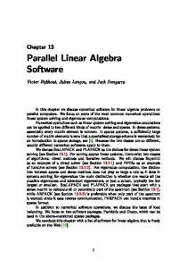
Figure 1: ATLAS’s matmul kernel search 3.4
Overview of ATLAS GEMM Kernel Search
ATLAS’s matmul kernel search is outlined in Figure 1. Our master search first calls the generator search, which uses a heuristic to probe the essentially unbounded optimization space allowed by the source generator, and returns the parameters (eg., blocking factor, unrollings, etc) of the best case found. The master search then calls the multiple implementation search, which simply times each hand-written matmul kernel in turn, returning the best. The best performing (generated, hand-tuned) kernel is then taken as our systemspecific L1 cache-contained kernel. Both multiple implementation and generator searches pass the requisite kernel through a timing step, where the kernel is linked with a AEOS-quality timer, and executed on the actual hardware. Once the search completes, the chosen kernel is then tested to ensure it is giving correct results, as a simple sanity test to catch errors in compilation or kernels. For both searches, our approach takes in some initial (empirically discovered) information such as L1 cache size, types of instructions available, types of assembly supported, etc, to allow for an up-front winnowing of the search space. The timers are structured so that operations have a large granularity, leading to fairly repeatable results even on non-dedicated machines. All results are stored in files, so that subsequent searches will not repeat the same experiments, allowing searches to build on previously obtained data. This also means that if a search is interrupted (for instance due to a machine failure), previously run cases will not need to be re-timed. A typical install takes from 1 to 2 hours for each precision. The first step of the master search probes for the size of the L1 cache. This is used to limit the search for NB , which is further restricted to a maximal size of 80 in order to main10
tain performance for applications such as the LAPACK factorizations, which partially rely on unblocked computations. Similar small benchmarks are used to determine the maximal number of registers and the correct floating point operations to use. This process is described in greater detail in [2]. When both the multiple implementation and generator searches are completed, the master search designates the fastest of these two kernels (generated and hand-written) as the architecture-specific kernel for the target machine, and it is then leveraged to speed up the entire Level 3 BLAS, as we have previously discussed. 3.5
Source Generator Details
The source generator is the key to ATLAS’s portable efficiency. As can be seen from Figure 1, the code generator is completely platform independent, as it generates only strict ANSI/ISO C. It takes in parameters, which together optimize for instruction and data cache utilization, software pipelining, register blocking, loop unrolling, dependence breaking, superscalar & fetch scheduling, etc. Note that since the generated source is C, we can always use the compiler’s version of a particular transformation if it is highly optimized. For instance, a kernel generated with no inner-loop unrolling may be the best, because the compiler itself unrolls the inner loop, etc. Thus, the source generator’s optimizations are essentially the union of the optimizations it and the native compiler possess. The most important options to the source generator are: • Size of L1 cache block, NB • Support for A and/or B being either standard form, or stored in transposed form • Register blocking of “outer product” form (the most optimal form of matmul register blocking). Varying the register blocking parameters provides many different implementations of matmul. The register blocking parameters are: – ar : registers used for elements of A, – br : registers used for elements of B Outer product register blocking then implies that ar × br registers are then used to block the elements of C. Thus, if Nr is the maximal number of registers discovered during the floating point unit probe, the search will try essentially all ar and br that satisfy ar br + ar + br ≤ Nr . • Loop unrollings: There are three loops involved in matmul, one over each of the provided dimensions (M, N and K), each of which can have its associated unrolling factor (mu , nu , ku ). The M and N unrolling factors are restricted to varying with the associated register blocking (ar and br , respectively), but the K-loop may be unrolled to any depth (i.e., once ar is selected, mu is set as well, but ku is an independent variable). • Choice of floating point instruction: – combined multiply/add with associated scalar expansion – separate multiply and add instructions, with associated software pipelining and scalar expansion • User choice of utilizing generation-time constant or run-time variables for all loop dimensions (M, N, and K; for non-cleanup copy L1 matmul, M = N = K = NB ). For each dimension that is known at generation, the following optimizations are made: – If unrolling meets or exceeds the dimension, no actual loop is generated (no need for loop if fully unrolled).
11
–
•
If unrolling is greater than one, correct cleanup can be generated without using an if (thus avoiding branching within the loop). Even if a given dimension is a run-time variable, the generator can be told to assume particular, no, or general-case cleanup for arbitrary unrolling. For each operand array, the leading dimension can be a run-time variable or a generationtime constant (for example, it is known to be NB for copied L1 matmul), with associated savings in indexing computations For each operand array, the leading dimension can have a stride (stride of 1 is most common, but stride of 2 can be used to support complex arithmetic). The generator can eliminate unnecessary arithmetic by generating code with special α (1, -1, and variable) and β (0, 1, -1, and variable) cases. In addition, there is a special case for when α and β are both variables, but it is safe to divide β by α (this can save multiple applications of α). Various fetch patterns for loading A and B registers
3.6
The Importance of Multiple Implementation
•
• •
With the generality of the source generator coupled with modern optimizing compilers, it may seem counter-intuitive that multiple implementation is needed. Because ATLAS is open source, however, multiple implementation can be very powerful. We have designed the matmul kernel to be simple, and provided the infrastructure so that a user can test and time hand-tuned implementations of it easily (see [24] for details). This allows any interested user to write the kernel as specifically as required for the architecture of interest, even including writing in assembly (as shown in Figure 1). This then allows for the exploitation of architectural features which are not well utilized by the compiler or the source generator which depends upon it. Our own experience has been that even the most efficient compiled kernel can be improved by a modest amount (say around 5%) when written by a skilled hand-coder in assembly, due merely to a more efficient usage of system resources than general-purpose compilers can achieve on complicated code. This problem became critical with the widespread availability of SIMD instructions such as SSE. At first, no compiler supported these instructions; now a few compilers, such as Intel’s icc, will do the SIMD vectorization automatically, but they still cannot do so in a way that is competitive with hand-tuned codes for any but the simplest of operations. For example, on a Pentium 4, if ATLAS is installed using the Intel’s compilers, the best multiple implementation kernel is 1.9 (3.1) times faster than the best DGEMM (SGEMM, respectively) created using source generation. The main differences between the handtuned kernels and the generated kernels is that they fully exploit SSE (including using prefetch). Therefore, multiple implementation is very useful as a mechanism to capture optimizations that the compiler and generator cannot yet fully exploit. Since ATLAS never blindly uses even a kernel written specifically for a particular architecture, as greater capabilities come online upstream (for instance, better SIMD vectorization in the compiler, or source generation of SIMD assembly), the search will continue to get the best of both worlds. Note that it may seem that these kernels might be good for only one machine, but this is certainly not true in practice, as even a kernel written in assembly may still be an aid to persistent optimization. For instance, a kernel optimized for the Pentium III might be the best available implementation for the Pentium IV or Athlon as well.
12
4
Automatically Tuned Numerical Kernels: the Sparse Case
This section reviews our recent work on automatic tuning of computational kernels involving sparse matrices (or, sparse kernels) [30, 31, 32, 33, 34]. Like the dense kernel case described above in Section 2.2, tuning sparse kernels is difficult owing to the complex ways in which performance depends on the underlying machine architecture. In addition, performance in the sparse case depends strongly on the non-zero structure of the user’s sparse matrix. Since the matrix might not be known until run-time, decisions about how to apply memory hierarchy optimizations like register- and cache-level blocking (tiling) transformations must be deferred until run-time. Since tuning in the dense case can be performed off-line (e.g., as in ATLAS [2]), the need for run-time tuning is a major distinction of the sparse case. Below, we show examples of the difficulties that arise in practice (Section 4.1), describe how our hybrid off-line/run-time empirical approach to tuning addresses these difficulties (Section 4.2), and summarize the optimization techniques we have considered for sparse kernels (Section 4.3). This work is being implemented in the S PARSITY Version 2 automatic tuning system [30, 35]. This system builds on a successful prototype (S PARSITY Version 1 [36]) for generating highly tuned implementations of one important sparse kernel, sparse matrix-vector multiply (SpMV). The work described here expands the list of optimizations that S PARSITY can consider (Section 4.3.1), and adds new sparse kernels such as sparse triangular solve (Section 4.3.2). 4.1
Challenges and Surprises in Tuning
Achieving high-performance for sparse kernels requires choosing appropriate data structure and code transformations that best exploit properties of both the underlying machine architecture (e.g., caches and pipelines) and the non-zero structure of the matrix. However, non-obvious choices often yield the most efficient implementations due to the surprisingly complex behavior of performance on modern machines. We illustrate this phenomenon below, after a brief review of the basics of sparse matrix storage. 4.1.1 Overheads Due to Sparse Data Structures Informally, a matrix is sparse if it consists of relatively few non-zeros. We eliminate storage of and computation with the zero entries by a judicious choice of data structure which stores just the non-zero entries, plus some additional indexing information to indicate which nonzeros have been stored. For instance, a typical data structure for storing a general sparse matrix is the so-called compressed sparse row (CSR) format, which is the baseline format in standard libraries such as SPARSKIT [37] and PETSc [38].1 The CSR data structure packs the non-zero values of the matrix row by row in an array. CSR stores an additional integer column index for each non-zero in a second parallel array, and maintains a third array holding pointers to the start of each row within the value and index arrays. Compared to dense matrix storage, CSR has a per non-zero overhead of 1 integer index (ignoring the row pointers). The resulting run-time overheads are significant for sparse kernels like SpMV. Consider the SpMV operation y ← y + A · x, where A is a sparse matrix and x, y are dense vectors. This operation executes only 2 flops per non-zero of A, (Section 3), and the elements of 1. Sparse matrices in the commercial engineering package, MATLAB, are stored in the analogous compressed sparse column (CSC) format [39].
13
Matrix 02−raefsky3
0
0
Matrix 02−raefsky3: 8x8 blocked submatrix (1:80, 1:80)
8
2656
16
5312
24
7936
32 40
10592
48
13248
56 15904
64 18560 21216 0
72 2656
5312
7936 10592 13248 15904 18560 21216 80 0 1.49 million non−zeros
8
16
24
32
40
48
56
64
72
80
Figure 2: Example of a sparse matrix with simple block structure: (Left) A sparse matrix arising from a finite element discretization of an object in a fluid flow simulation. This matrix has dimension n = 21216 and contains approximately 1.5 million non-zeros. (Right) The matrix consists entirely of 8×8 dense non-zero blocks, uniformly aligned as shown in this 80×80 submatrix. A are not reused. Thus, there is little opportunity to hide the cost of extra loads due to the column indices. In addition, sparse data structures lead to code with indirect memory references, which can be difficult for compilers to analyze statically. For example, CSR storage prevents automatically tiling accesses to x for either registers or caches, as might be done in the dense case [40, 41, 42, 43]. Depending on the matrix non-zero structure, the resulting memory access patterns can also be irregular—for CSR, this possibility prevents hardware or software prefetching of the elements of x. 4.1.2 Surprising Performance Behavior in Practice We can reduce the sparse indexing overheads by recognizing patterns in the non-zero structure. For example, in simulations based on the finite element method, the matrix may consist entirely of small fixed size dense rectangular r×c blocks. We can used a blocked variant of CSR—block CSR, or BCSR, format—which stores one index per block instead of one per non-zero. Figure 2 shows an example of a sparse matrix which consists entirely of 8×8 blocks. This format enables improved scheduling and register-level reuse opportunities compared to CSR: multiplication in BCSR format proceeds block-by-block, where each r×c block multiply is fully unrolled and the corresponding r elements of y and c elements of x stored in registers. For this example matrix, BCSR reduces the overall index storage by a factor of r · c = 64 compared to CSR. Even if the block structure is simple and known, the best block size is not always obvious. For example, consider an experiment in which we executed 16 r×c BCSR implementations of SpMV on the matrix shown in Figure 2, where r, c ∈ {1, 2, 4, 8}. We show the results on a machine based on the Sun Ultra3 microprocessor in Figure 3 (left), and on the Intel Itanium 2 in Figure 3 (right). On each platform, each implementation is shaded by its performance in Mflop/s and labeled by its speedup relative to the CSR (or, unblocked 1×1) 14
900 MHz Ultra 3, Sun CC v6: ref=54 Mflop/s 8
1.68
1.80
1.89
2.04
900 MHz Itanium 2, Intel C v7.0: ref=275 Mflop/s
109 104 99
8
4.01
2.45
1.20
1.55
4
3.34
4.07
2.31
1.16
2
1.91
2.52
2.54
2.23
1
1.00
1.35
1.12
1.39
4
2
1.51
1.66
1.72
1.91
1.25
1.45
1.59
1.74
89 84 79 74 69
1
row block size (r)
row block size (r)
94
64
1.00 1
1.26 2
1.45 4
column block size (c)
1.57 8
59 54
1
2
4
column block size (c)
8
1120 1080 1030 980 930 880 830 780 730 680 630 580 530 480 430 380 330 280
Figure 3: Surprising performance behavior in practice: register blocked sparse matrixvector multiply. Each square is an r×c implementation, shaded by its performance in Mflop/s and labeled by its speedup relative to the unblocked (1×1) CSR implementation, where r, c ∈ {1, 2, 4, 8}. (Left) On the Sun Ultra3 platform (1.8 Gflop/s peak), performance increases smoothly as r, c increase, as expected. (Right) On the Intel Itanium 2 platform (3.6 Gflop/s peak), 31% of peak (4× speedup) is possible, but at 4×2 instead of 8×8. case. Observe that maximum speedups of 2.04× on the Ultra3 and 4.07× on the Itanium 2 are possible for this matrix. On the Itanium 2, this performance is over 1.1 Gflop/s, or 31% of peak machine speed, and is comparable to the performance of a well-tuned dense matrix-vector multiply performance (DGEMV) of 1.3 Gflop/s by Goto [44]. However, the best block size is 4×2, and not 8×8 on Itanium 2. Although there are a variety of reasons why users might reasonably expect performance to increase smoothly as r×c increases toward 8×8—as it does on the Ultra3—the irregular variation in performance observed on the Itanium 2 is typical on a wide range of modern machines [31]. Indeed, this kind of behavior persists even if we remove all of the irregularity in the memory access pattern by, for instance, using a dense matrix stored in BCSR format [31]. The problem of data structure selection is further complicated by the fact that we can alter the non-zero pattern by introducing explicit zeros to enable the use of a fast implementation. For example, consider the sparse matrix shown in Figure 4 (left), which has a complex arrangement of non-zeros (each shown as a dot). There is no obvious single r×c block size that perfectly captures this structure. Suppose we nevertheless store the matrix in 3×3 format, as shown in Figure 4 (right), storing explicit zeros (each shown as an ’x’) to fill each block. We define the fill ratio at r×c to be the total number of stored zeros (original nonzeros plus explicit zeros) divided by the number of original non-zeros. In this example, the fill ratio at 3×3 happens to be 1.5, meaning that SpMV in this format will execute 1.5 times as many flops. However, the resulting implementation on a Pentium III takes 32 as much time as the unblocked implementation (a 1.5× speedup). In general, this speedup is possible because (a) though the flops increase, index storage (and possibly total storage) can be reduced, and (b) implementations at particular values of r and c may be especially efficient, as we suggested by the Itanium 2 results shown in Figure 3 (right). There are many additional examples of complex and surprising performance behavior, and we refer the interested reader to recent work documenting these phenomena [31, 30, 35].
15
Before Register Blocking: Matrix 13−ex11
After 3x3 Register Blocking: Matrix 13−ex11
0
0
3
3
6
6
9
9
12
12
15
15
18
18
21
21
24
24
27
27
30
30
33
33
36
36
39
39
42
42
45
45
48 51
48 0
3
6
9 12 15 18 21 24 27 30 33 36 39 42 45 48 51 715 ideal nz
51
0
3
6
9 12 15 18 21 24 27 30 33 36 39 42 45 48 51 715 ideal nz + 356 explicit zeros = 1071 nz
Figure 4: Altering the non-zero pattern can yield a faster implementation: (Left) A 50×50 submatrix of Matrix ex11 from a fluid flow problem [45]. Non-zeros are shown by dots. (Right) The same matrix stored in 3×3 BCSR format. We impose a logical grid of 3×3 cells, and fill in explicit zeros (shown by x’s) to ensure that all blocks are full. The fill ratio for the entire matrix is 1.5, but the SpMV implementation is still 1.5 times faster than the unblocked case on a Pentium III platform. Despite the 50% increase in stored values, total storage (in bytes) increases only by 7% because of the reduction in index storage. 4.2
A Hybrid Off-line/Run-time Empirical Search-Based Approach to Tuning
Our approach to choosing an efficient data structure and implementation, given a kernel, sparse matrix, and machine, is based on a combination of heuristic performance modeling and experiments, carried out partly off-line and partly at run-time. For each kernel, we 1. identify and generate a space of reasonable implementations, and 2. search this space for the best implementation using a combination of heuristic models and experiments (i.e., actually running and timing the code). For a particular sparse kernel and matrix, the implementation space is a set of data structures and corresponding implementations (i.e., code). Each data structure is designed to improve locality by exploiting a class of non-zero patterns commonly arising in practice, such as small fixed-sized rectangular blocks, diagonals and bands, or symmetry, or even combinations of these patterns. Section 4.3 summarizes the kinds of performance improvements we have observed on a variety of different architectures for several locality-enhancing data structures and algorithms. We search by evaluating heuristic models that combine benchmarking data with estimated properties of the matrix non-zero structure. The benchmarks, which consist primarily of executing each implementation (data structure and code) on synthetic matrices, need to be executed only once per machine. This step characterizes the machine in a matrix-independent way. When the user’s sparse matrix is known at run-time, we estimate performance-relevant structural properties of the matrix. The heuristic models combine these benchmarking and matrix-specific data to predict what data structure will yield the best performance. This approach uses both modeling and experiments, both off-line and at run-time. Below, we
16
describe an example of this methodology applied to the selection of register-level block (tile) sizes for SpMV and other sparse kernels. 4.2.1 Example: Using Empirical Models and Search to Select a Register Block Size We can overcome the difficulties in selecting a register block size discussed in Section 4.1 using the following empirical technique. The basic idea is to decouple machine-specific aspects of performance which can be measured off-line from matrix-specific aspects determined at run-time. In the example of Figures 2–3, trying all or even a subset of block sizes is likely to be infeasible if the matrix is known only at run-time, because of the cost of simply converting the matrix to blocked format. For instance, the cost of converting a matrix from CSR format to BCSR format once can be as high as 40 SpMVs in CSR format, depending on the platform and matrix [31]. Though the cost of a single conversion is acceptable in many important application contexts (e.g., solving linear systems or computing eigenvalues by iterative methods) where hundreds or thousands of SpMVs can be required for a given matrix, exhaustive run-time search—needed particularly in the case when we may allow for fill of explicit zeros in blocking, for example—is still likely to be impractical. Our goal then is to develop a procedure for selecting an r×c block size that is reasonably accurate, requires at most a single conversion, and whose cost is small compared to the cost of conversion. The irregularity of performance as a function of r and c means that developing an accurate but simple analytical performance model will be difficult. Instead, we use the following three-step empirical procedure: 1. Off-line benchmark: Once per machine, measure the speed (in Mflop/s) of r×c register blocked SpMV for a dense matrix stored in sparse format, at all block sizes from 1×1 to 12×12. Denote the register profile by {Prc (dense) |1 ≤ r, c ≤ 12}. 2. Run-time “search”: When the matrix A is known at run-time, compute an estimate fˆrc (A) of the true fill ratio for all 1 ≤ r, c, ≤ 12. This estimation constitutes a form of empirical search over possible block sizes. 3. Heuristic performance model: Choose r, c that maximizes the following estimate of register blocking performance Pˆrc (A), Prc (dense) (1) Pˆrc (A) = fˆrc (A) This model decouples machine-specific aspects of performance (register profile in the numerator) from a matrix-specific aspect (fill ratio in the denominator). This procedure, implemented in the upcoming release of S PARSITY, frequently selects the best block size, and yields performance that is nearly always 90% or more of the best [30, 31]. In addition, the run-time costs of steps 2 and 3 above can be kept to between 1–11 unblocked SpMVs, depending on the platform and matrix, on several current platforms [31]. This cost is the penalty for evaluating the heuristic if it turns out no blocking is required. If blocking is beneficial, we have found that the overall block size selection procedure including conversion is never more than 42 1×1 SpMVs on our test machines and matrices, meaning the cost of evaluating the heuristic is modest compared to the cost of conversion [31]. Moreover, we can easily generalize this heuristic procedure for other kernels by simply substituting a kernel-specific register profile (step 1). We have shown that this procedure selects optimal or near-optimal block sizes for sparse triangular solve [46] and multiplication by AAT [47]. 17
4.2.2 Contrast to a Static Compilation Approach There are several aspects of our approach to tuning sparse kernels which are beyond the scope of traditional static general-purpose compiler approaches. • Transformations based on run-time data: For a particular sparse matrix, we may choose a completely different data structure from the initial implementation; this new data structure may even alter the non-zero structure of the matrix by, for example, reordering the rows and columns of the matrix, or perhaps by choosing to store some zero values explicitly (Section 4.1). These kinds of transformations depend on the run-time contents of the input matrix data structure, and these values cannot generally be predicted from the source code implementation alone. • Aggressive exploitation of domain-specific mathematical properties for performance: In identifying the implementation spaces, we consider transformations based on mathematical properties that we would not expect a general purpose compiler to recognize. For instance, in computing the eigenvalues of A using a Krylov method [48], we may elect to change A to P · A · P T , where P is a permutation matrix. This permutation of rows and columns may favorably alter the non-zero structure of A by improving locality, but mathematically does not change the eigenvalues, and therefore the application of P may be ignored. • Heuristic, empirical models: Our approach to tuning identifies candidate implementations using heuristic models of both the kernel and run-time data. We would expect compilers built on current technology neither to identify such candidates automatically, nor posit the right models for choosing among these candidates. We elaborate on this argument elsewhere [31]. • Tolerating the cost of search: Searching has an associated cost which can be much longer than traditional compile-times. Knowing when such costs can be tolerated, particularly since these costs are incurred at run-time, must be justified by actual application behavior. This behavior can be difficult to deduce with sufficient precision based on the source code alone. 4.3
Summary of Optimization Techniques and Speedups
We have considered a variety of performance optimization techniques for sparse kernels in addition to the register-level blocking scheme described in Section 4.2 [30, 31, 32, 33, 34]. Below, we summarize these techniques, reporting the maximum speedups over CSR and register blocking that we have observed for each technique. We also note major unresolved issues, providing pointers both to existing and upcoming reports that discuss these techniques in detail and to related work external to this particular research project. At present, we are considering all of these techniques for inclusion in the upcoming release of S PAR SITY . We have evaluated these techniques on a set of 44 test matrices that span a variety of applications domains. For our summary, we categorize these matrices into three broad classes as follows: • Single-block FEM Matrices: These matrices, arising in finite element method (FEM) applications, have non-zero structure that tends to be dominated by a single block size on a uniformly aligned grid. The matrix shown in Figure 2 exemplifies this class of matrix structures. • Multi-block FEM Matrices: These matrices also arise in FEM applications, but have a non-zero structure that can be characterized as having one or more “natural”
18
block sizes aligned irregularly. Figure 4 shows one example of a matrix from this class, and we mention another below. • Non-FEM Matrices: We have also considered matrices arising in a variety of NonFEM based modeling and simulation, including oil reservoir modeling, chemical process simulation, finance and macroeconomic modeling, and linear programming problems, among others. The main distinction of this class is the lack of regular block structure, though the non-zero structure is generally not uniformly random, either. This categorization reflects the fact that the register blocking optimization, the technique we have most thoroughly studied among those listed below, appears to yield the best absolute performance in practice on cache-based superscalar platforms. 4.3.1 Techniques for Sparse Matrix-Vector Multiply The following list summarizes the performance-enhancing techniques we have considered specifically for SpMV. Full results and discussion can be found in [31]. •
Register blocking, based on BCSR storage: up to 4× speedups over CSR. A number of recent reports [30, 31, 35, 36] validate and analyze this optimization in great depth. The largest pay-offs occur on Single-block FEM matrices, where we have observed speedups over CSR of up to 4×. We have also observed speedups of up to 2.8× on Multi-block FEM matrices by judicious creation of explicit zeros as discussed for the matrix in Figure 4. The accuracy of the block size selection procedure described in Section 4.2 means we can apply this optimization fully automatically.
•
Multiplication by multiple vectors: up to 7× over CSR, up to 2.5× over register blocked SpMV. Some applications and numerical algorithms require applying the matrix A to many vectors simultaneously, i.e., the “SpMM” kernel Y ← Y + A · X, where X and Y are dense matrices [36, 49]. We can reuse A in this kernel, where the key tuning parameter is the depth of unrolling across the columns of X and Y .
•
Cache blocking: up to 2.2× over CSR. Cache blocking, as described in implemented by Im [36] for SpMV, reorganizes a large sparse matrix into a collection of smaller, disjoint rectangular blocks to improve temporal access to elements of x. This technique helps to reduce misses to the source vector toward the lower bound of only cold start misses. The largest improvements occur on large, randomly structured matrices like those arising in linear programming applications, and in latent semantic indexing applications [50].
•
Symmetry: symmetric register blocked SpMV is up to 2.8× faster than nonsymmetric CSR SpMV, and up to 2.1× faster than non-symmetric register blocked SpMV; symmetric register blocked SpMM is up to 7.3× faster than CSR SpMV, and up to 2.6× over non-symmetric register blocked SpMM. Lee, et al., study a register blocking scheme when A is symmetric (i.e., A = AT ) [32]. Symmetry requires that we only store roughly half of the non-zero entries, and yields significant performance gains as well.
•
Variable block splitting, based on unaligned BCSR storage: up to 2.1× over CSR; up to 1.8× over register blocking. To handle the Multi-block FEM matrices, which are composed of multiple irregularly aligned rectangular blocks, we have considered a technique in which we split 19
the matrix A into a sum A = A1 + A2 + . . . + As , where each term is stored in an unaligned BCSR (UBCSR) data structure. UBCSR augments BCSR format with additional indices that allow for arbitrary row alignments [31]. The split-UBCSR technique reduces the amount of fill compared to register blocking. The main matrixand machine-specific tuning parameters in the split UBCSR implementation are the number of splittings s and the block size for each term Ai . We view the lack of a heuristic for determining whether and how to split to be the major unresolved issue related to splitting. •
Exploiting diagonal structure, based on row-segmented diagonal storage: up to 2× over CSR. Diagonal formats (and diagonal-like formats, such as jagged-diagonal storage [37]) have traditionally been applied on vector architectures [51, 52]. We have shown the potential pay-offs from careful application on superscalar cache-based microprocessors by generalizing diagonal format to handle complex compositions of non-zero diagonal runs [31]. For example, Figure 5 shows a submatrix of a larger matrix with diagonal run substructure. The rows between each pair of consecutive horizontal lines consists of a fixed number of diagonal runs. By storing the matrix in blocks of consecutive rows as shown and unrolling the multiplication along diagonals, we have shown that implementations based on this format can lead to speedups of 2× or more for SpMV, compared to a CSR implementation. The unrolling depth is the main matrix- and machine-specific tuning parameter. Again, effective heuristics for deciding when and how to select the main matrix- and machine-specific tuning parameter (unrolling depth) remain unresolved. However, our preliminary data suggests that performance is a relatively smooth function of the tuning parameter, compared to the way in which performance varies with block size, for instance [31]. This finding suggests that a practical heuristic will not be difficult to develop.
•
Reordering to create dense blocks: up to 1.5× over CSR. Pinar and Heath proposed a method to reorder rows and columns of a sparse matrix to create dense rectangular block structure which might then be exploited by splitting [53]. Their formulation is based on the Traveling Salesman Problem. In the context of S PARSITY, Moon, et al., have applied this idea to the S PARSITY benchmark suite, showing speedups over conventional register blocking of up to 1.5× on a few of the Multi-block FEM and Non-FEM matrices.
4.3.2 Techniques for Other Sparse Kernels A variety of optimization techniques may be applied to sparse kernels besides SpMV, as summarized below. •
Sparse triangular solve: up to 1.8× speedups over CSR. We recently showed how to exploit the special structure of sparse triangular matrices that arise during LU factorization [46]. These matrices typically have a large dense trailing triangle, such as the one shown in Figure 6: The trailing triangle in the lower right-hand corner of this lower triangular matrix accounts for more than 90% of the total non-zeros. We partition the solve into a sparse phase and a dense phase by appropriate algorithmic and data structure reorganizations. To the sparse phase, we adapt the register blocking optimization as it is applied to SpMV; to the dense phase, we can call a tuned BLAS triangular solve routine (e.g., DTRSV). We refer to this 20
0
mc2depi.rua: 2D epidemiology study (Markov chain) [n=525825]
10 20 30 40 50 60 70 80 0
10
20 30 40 50 60 nnz shown = 278 [nnz(A) = 2100225]
70
80
Figure 5: An example of complex diagonal structure: An 80×80 submatrix of a larger matrix that arises in an epidemiology study [54]. All of the rows between each pair of consecutive horizontal lines intersect the same diagonal runs. latter step as the switch-to-dense optimization. Like register blocking for SpMV, the process of identifying the trailing triangle and selecting a block size can be fully automated [46]. We have observed performance improvements of up to 1.8× over a basic implementation of sparse triangular solve using CSR storage. •
Multiplication by sparse AAT : 1.5−4.2× relative to applying A and AT in CSR as separate steps; up to 1.8× faster than BCSR. The kernel y ← y+AAT ·x, where A is a given sparse matrix and x, y are dense vectors, is a key operation in the inner-loop of interior point methods for mathematical programming problems [55], algorithms for computing the singular value decomposition [48], and Kleinberg’s HITS algorithm for finding hubs and authorities in graphs [56], among others. A typical implementation first computes t ← AT · x followed by y ← y + A · t. Since A will generally be much larger than the size of the cache, the elements of A will be read from main memory twice. However, we can reorganize the computation to reuse A.
•
Multiplication by sparse Ak using serial sparse tiling: when k = 4, up to 2× faster than separately applying A k times in BCSR format. Like AAT · x, the kernel y ← Ak · x, which appears in simple iterative algorithms like the power method for computing eigenvalues [48], also has opportunities to reuse elements of A. A typical reference implementation stores A in CSR or BCSR format, and separately applies A k times.
4.4
Remaining Challenges and Related Work
Although pay-offs from individual techniques can be significant, the common challenge is deciding when to apply particular optimizations and how to choose the tuning parameters. While register blocking and automatic block size selection is well understood for SpMV, sparse triangular solve, and multiplication by sparse AAT , heuristics for the other 21
Figure 6: The non-zero structure of a sparse triangular matrix arising from LU factorization: This matrix, from the LU factorization of a circuit simulation matrix, has dimension 17758 and 2 million non-zeros. The trailing triangle, of dimension 1978, is completely dense and accounts for over 90% of all the non-zeros in the matrix. optimization techniques still need to be developed. The Non-FEM matrices largely remain difficult, with exceptions noted above (also refer to a recent summary for more details [31]). Careful analysis using performance bounds models indicates that better low-level tuning of the CSR (i.e., 1 × 1 register blocking) SpMV implementation may be possible [31]. Recent work on low-level tuning of SpMV by unroll-and-jam (Mellor-Crummey, et al. [57]), software pipelining (Geus and R¨ollin [58]), and prefetching (Toledo [59]) are promising starting points. Moreover, expressing and automatically applying these low-level optimizations is a problem shared with dense matrix kernels. Thus, low-level tuning of, say, each r×c implementation in the style of ATLAS and PHiPAC may yield further performance improvements for sparse kernels. It is possible that by performing an ATLAS style search over possible instruction schedules may smooth out the performance irregularities shown in Figure 3 (right). It may be possible to modify existing specialized restructuring compiler frameworks for sparse code generation to include an ATLAS-style search over possible instruction schedules [60, 61, 62]. In the space of higher-level sparse kernels beyond SpMV and triangular solve, the sparse triple product, or RART where A and R are sparse matrices, is a bottleneck in the multigrid solvers [63, 64, 65, 66]. There has been some work on the general problem of multiplying sparse matrices [67, 68, 69, 70], including recent work in a large-scale quantum chemistry application that calls matrix-multiply kernels automatically generated and tuned by PHiPAC for particular block sizes [71, 1]. This latter example suggests that a potential opportunity to apply tuning ideas to the sparse triple product kernel.
22
5
Statistical determination of numerical algorithms
In the previous sections we looked at tuning numerical kernels. One characteristic of the approach taken is that the analysis can be performed largely statically, that is, with most of the analysis taking place at installation time. The tuned dense kernels then are almost independent of the nature of the user data, with at most cases like very ‘skinny’ matrices handled separately; tuned sparse kernels have a dynamic component where the tiling and structuring of the matrices is at run-time handled, but even there the numerical values of the user data are irrelevant. Algorithm choice, the topic of this section, is an inherently more dynamic activity where the numerical content of the user data is of prime importance. Abstractly we could say that the need for dynamic strategies here arises from the fact that any description of the input space is of a very high dimension. In the case of dense and sparse kernels, the algorithm search space is considerable, but the input data is easy to describe. For dense kernels at most we allow for decisions based on matrix size (for instance, small or ‘skinny’ matrices); for sparse matrices we need some description of the nonzero density of the matrix to gauge the fill-in caused by blocking strategies. The input in such applications as linear system solving is much harder to describe: we would typically need to state the nonzero structure of the system, various norm-like properties, and even spectral characteristics of the system. As a corollary, we can not hope to exhaustively search this input space, and we have to resort to some form of modeling of the parameter space. We will give a general discussion of the issues in dynamic algorithm selection and tuning, present our approach which uses statistical data modeling, and give some preliminary results obtained with this approach. 5.1
Dynamic Algorithm Determination
In finding the appropriate numerical algorithm for a problem we are faced with two issues: 1. There are often several algorithms that, potentially, solve the problem, and 2. Algorithms often have one or more parameters of some sort. Thus, given user data, we have to choose an algorithm, and choose a proper parameter setting for it. Numerical literature is rife with qualitative statements about the relative merits of methods. For instance, augmenting GMRES with approximated eigenvectors speeds convergence in cases where the departure from normality of the system is not too large [72]. It is only seldom that quantitative statements are made, such as the necessary restart length of GMRES to attain a certain error reduction in the presence of an indefinite system [73]. Even in this latter case, the estimate derived is probably far from sharp. Thus we find ourselves in the situation that the choice between candidate methods and the choice of parameter settings can not, or only very approximately, be made by implementing explicitly known numerical knowledge. However, while making the exact determination may not be feasible, identifying the relevant characteristics of an application problem may be possible. Instead of implementing numerical decisions explicitly, we can then employ statistical techniques to identify correlations between characteristics of the input, and choices and parametrizations of the numerical methods. Our strategy in determining numerical algorithms by statistical techniques is globally as follows. • We solve a large collection of test problems by every available method, that is, every choice of algorithm, and a suitable ‘binning’ of algorithm parameters. 23
•
Each problem is assigned to a class corresponding to the method that gave the fastest solution. • We also draw up a list of characteristics of each problem. • We then compute a probability density function for each class. As a result of this process we find a function pi (¯ x) where i ranges over all classes, that is, all methods, and x ¯ is in the space of the vectors of features of the input problems. Given a new problem and its feature vector x ¯, we then decide to solve the problem with the method i for which pi (¯ x) is maximised. We will now discuss the details of this statistical analysis, and we will present some proofof-concept numerical results evincing the potential usefulness of this approach. 5.2
Statistical analysis
In this section we give a short overview of the way a multi-variate Bayesian decision rule can be used in numerical decision making. We stress that statistical techniques are merely one of the possible ways of using non-numerical techniques for algorithm selection and parameterization, and in fact, the technique we describe here is only one among many possible statistical techniques. We will describe here the use of parametric models, a technique with obvious implicit assumptions that very likely will not hold overall, but, as we shall show in the next section, they have surprising applicability. 5.2.1 Feature extraction The basis of the statistical decision process is the extraction of features2 from the application problem, and the characterization of algorithms in terms of these features. In [74] we have given examples of relevant features of application problems. In the context of linear/nonlinear system solving we can identify at least the following categories of features: • Structural characteristics. These pertain purely to the nonzero structure of the sparse problem. While at this level the numerical properties of the problem are invisible, in practice the structure of a matrix will influence the behaviour of such algorithms as incomplete factorisations, since graph properties are inextricably entwined with approximation properties. • Simple numerical characteristics. By these we mean quantities such as norms (1norm, infinity norm, norm of symmetric part, et cetera) that are exactly calculable in a time roughly proportional to the number of nonzeros of the matrix. • Spectral properties. This category includes such characteristics as the enclosing ellipse of the field of values, or estimates of the departure from normality. While such quantities are highly informative, they are also difficult, if not impossible, to calculate in a reasonable amount of time. Therefore, we have to resort to approximations to them, for instance estimating the spectrum from investigating the Hessenberg reduction after a limited-length Krylov run [75, 76]. A large number of such characteristics can be drawn up, but not all will be relevant for each numerical decision. After the testing phase (described below), those features that actually correlate with our decisions will have to be found. Also, many features need to be normalized somehow, for instance relating structural properties to the matrix size, or numerical properties to some norm of the matrix or even the (1, 1) element of the matrix. 2. We use the terms ‘characteristics’ and ‘features’ interchangably, ‘features’ being the term used in the statistical literature.
24
5.2.2 Training stage Based on the feature set described above, we now engage in an – expensive and timeconsuming – training phase, where a large number of problems is solved with every available method. For linear system solving, methods can be described as an orthogonal combination of several choices: • Iterative method. The choice of iterative method entails both the choice between such different methods as BiCGstab [77] and GMRES [73], and the choice of parameters such as the restart length of GMRES. In order to make the latter choice manageable, we ‘bin’ the possible values, in effect limiting it to a few values that we predict to be practically qualitatively different. For instance, for the GMRES parameter we only investigate the choices 5, 20, 50. • Preconditioner. This is probably the most important choice in constructing an iterative linear system solver. While there are theoretical statements about relations between iterative methods, no such knowledge about preconditioners exists. In fact, for each pair of preconditioners we can find problems where one is suitable and the other not. As in the case of iterative methods, we may need to bin method parameters, for instance the number of ILU fill-in levels. • Scaling, permutation, and other preprocessing steps. While the above choices of deciding the iterative method and preconditioner are the ones that mostly come to mind when we talk about iterative solvers, there are various preprocessing steps one can apply to the problem that can have a large influence on convergence speed. In fact, for our numerical test below we investigate the influence of different permutations of the linear system on the speed of solution. In spite of this multi-dimensional characterization of iterative solvers, we will for the purpose of this exposition consider methods as a singly-indexed set. The essential step in the training process is that each numerical problem is assigned to a class, where the classes correspond to the solvers, and the problem is assigned to the class of the method that gave the fastest solution. As a result of this, we find for each method (class) a number of problems that are best solved by it. From the feature vectors of these problems we extract a vector of mean values µ ¯ and a covariance matrix Σ: Σ=
N 1 X (¯ xi − µ)(¯ xi − µ)t N i=1
where {¯ xi }N i=1 are the samples in the class for which we are calculating the covariance matrix. The mean value vector and covariance matrix give us a multivariate density function for method j: −1 1 e−(1/2)(¯x−¯µ)Σ (¯x−¯µ) pj (¯ x) = 1/2 2π|Σ| Having computed these density functions, we can compute the a posteriori probability of a class (‘given a sample x ¯, what is the probability that it belongs in class j’) as P (wi |¯ x) =
p(¯ x|wj )P (wj ) . p(¯ x)
We then select the numerical method for which this quantity is maximised.
25
5.3
Numerical test
To study the behavior and performance of the statistical techniques described in the previous section, we perform several tests on a number of matrices from different sets from the Matrix Market [78]. To collect the data, we generate matrix statistics by running an exhaustive test of the different coded methods and preconditioners; for each of the matrices we collect statistics for each possible existing combination of: permutation, scaling, preconditioner and iterative method. From this data we select those combinations that converged and had the minimum solving time (those combinations that didn’t converge are discarded). Each possible combination corresponds to a class, but since the number of these combination is too large, we reduce the scope of the analysis and concentrate only on the behavior of the possible permutation choices. Thus, we have three classes corresponding to the partitioning types: Induced the default Petsc distribution induced by the matrix ordering and the number of processors, Parmetis , using the Parmetis [79, 80] package, Icmk a heuristic [81] that, without permuting the system, tries to find meaningful split points based on the sparsity structure. Our test is to see if the predicted class (method) is indeed the one that yields minimum solving time for each case. 5.4
Technical Approach
Following the approach described in the previous section, we first extract a series of statistics and from these, select a set of features which are suitable for this type of method, e.g. Bayesian analysis requires that the majority of the values collected for a feature are at least slightly different from each other. Several combinations of differing numbers of features have been used in different instances. Some of these features used are structural and spectral statistics of the matrices: • Diagonal, number of non-zeros, bandwidth • Number of non-zeros • Bandwidth Left and Right • Number of possible split points found by the ICMK algorithm • Ellipse enclosing the (estimated) spectrum: X and Y axes, and coordinates of the center (xa, ya, xc and yc) • Positive-definiteness, again based on an estimated spectrum. The next step is to collect the training data, for which we randomly divide the totality of the data in two portions, 66% is used for training the classifier, and the rest is used for testing and validation. With this information we can then proceed to apply the classifiers for training. In these tests we have used two types of classifying methods: parametric and nonparametric. With a parametric classifier (also called ‘supervised method’) we estimate the parameters for a presumed probability distribution function such as the normal distribution, and we use this function as a basis for making decisions. The non-parametric classifier does not assume the existence of any specific probability distribution, the function is instead built specially from the collected data. The last stage is validation. In our case we use the 34% of the data corresponding to the testing set to evaluate the previously trained classifiers and decide, for each testing sample to which class it belongs. For both of types of classification methods, the decision is made
26
using the Bayes decision rule. To assess the performance of the classifiers, we compare the predicted class to the class that, from the original data, has the smallest run time, if they match then we call a hit and if they don’t we have a classification error. 5.5
Results
These results were obtained using the following approach for both training and testing the classifier: considering that Induced and Icmk are the same except for the Block-Jacobi case, if a given sample is not using Block-Jacobi it is classified as both Induced and Icmk, and if it is using Block-Jacobi then the distinction is made and it is classified as Induced or Icmk. For the testing set, the verification is performed with same criteria, for instance, if a sample from the class Induced is not using Block-Jacobi and is classified as Icmk by the classifier, is still counted as a correct classification (same for the inverse case of Icmk classified as Induced), however, if a sample from the Induced class is classified as Induced and was using block-jacobi, it is counted as a misclassification. The results for the different sets of features tested, are as follows: Features: non-zeros, bandwidth left and right,splits number, ellipse axes Parametric Non-Parametric Induced Class: 70% 60% Parmetis Class: 98% 73% Icmk Class: 93% 82% Features: diagonal, non-zeros, bandwidth left and right, splits number, ellipse axes and center Parametric Non-Parametric Induced Class: 70% 80% Parmetis Class: 95% 76% Icmk Class: 90% 90% Features: diagonal, non-zeros, bandwidth left and right, ellipse’s x-axis and center’s x-coordinate, positive-definiteness Parametric Non-Parametric Induced Class: 67% 77% Parmetis Class: 93% 73% Icmk Class: 91% 94% Features: non-zeros, bandwidth left and right, splits number Parametric Non-Parametric Induced Class: 81% 53% Parmetis Class: 95% 95% Icmk Class: 94% 61% Features: diagonal, non-zeros, bandwidth left and right, ellipse axes, positive-definiteness Parametric Non-Parametric Induced Class: 40% 60% Parmetis Class: 86% 73% Icmk Class: 45% 81% Features: diagonal, bandwidth left and right, ellipse’s center xcoordinate, positive-definiteness Parametric Non-Parametric Induced Class: 89% 81% 27
Parmetis Class: 97% 67% Icmk Class: 54% 86% It is important to note that although we have many possible features to choose from, there might not be enough degrees of freedom (i.e. some of these features might be corelated), so it is important to continue experimentation with other sets of features. The results of these tests might give some lead for further experimentation and understanding of the application of statistical methods on numerical data. We now evaluate the performance of these methods by analyzing the gain and loss of respectively predicting right and mispredicting. To estimate the pentalty of a misprediction, i.e. relative difference between the time that corresponds to the predicted class, and the real smallest time recorded; the average penalty, taken over the different combinations of parameters of several random trials is of 0.7 with a standard deviation of 0.6, the maximum being 2.2 and the minimum of 0.03. To estimate the gain of predicting correctly, we compute the ratio between the worse time observed and the time corresponding to the predicted method, the average gain factor is of 4.6, the maximum observed is of 20 and the minimum of 1.6. Furthermore, we estimate the gain of mispredicting, i.e. even if the wrong class was chosen, the time associated to it might still be better than the worse time observed, for this case we compute the ratio between the worse time and the time of the predicted class, the average is 2.1, with a maximum of 5.4 and a minimum of 1.4 observed. These tests and results are a first glance at the behavior of the statistical methods presented, and there is plenty of information that can be extracted and explored in other experiments and perhaps using other methods.
6
Conclusion
For the efficient solution of scientific problems on today’s advanced platforms, an application scientist can no longer rely on text book algorithms and reference implementations thereof. Both the choice of algorithm and the optimization of its implementation require a good deal of expertise, traditionally that of a trained computer scientist. It is not enough to rely on research in programming languages, compilers, software tools. In this paper we have explored approaches to automating the optimization tasks that traditionally were entrusted to human experts. For kernel optimization, we have presented the AEOS (Automated Empirical Optimization of Software) approach, of which ATLAS and PHiPAC are prime examples, for dense and sparse operations respectively. Through a combination of automatic code generation and hand-coded optimizations these packages deliver several factors improvement over what even the best of compilers can achieve on reference implementations. We have presented the SALSA package which uses statistical data modeling as a tool for automatic algorithm choice. Taken individually, the packages discussed here show great usefulness in their respective target areas. However, their general approaches can be extended to other areas. The results presented here show great promise for the future of portable adaptive high-performance libraries.
28
References [1] J. Bilmes, K. Asanovi´c, C. Chin, and J. Demmel, “Optimizing matrix multiply using PHiPAC: a portable, high-performance, ANSI C coding methodology,” in Proceedings of the International Conference on Supercomputing. Vienna, Austria: ACM SIGARC, July 1997. [2] R. C. Whaley, A. Petitet, and J. J. Dongarra, “Automated empirical optimization of software and the ATLAS project,” Parallel Computing, vol. 27, no. 1–2, pp. 3–35, 2001, also available as University of Tennessee LAPACK Working Note #147, UTCS-00-448, 2000 (www.netlib.org/lapack/lawns/lawn147.ps). [3] E. I. Foster and C. Kesselman, The Grid – Blueprint for a New Computing Infrastructure. San Francisco, CA: Morgan Kaufmann Publishers, Inc., 1998. [4] J. Dongarra and E. Grosse, “Distribution of Mathematical Software via Electronic Mail,” Communications of the ACM, vol. 30, no. 5, pp. 403–407, 1987. [5] J. Du Croz and M. Pont, “The development of a floating-point validation package,” in Proceedings of the 8th Symposium on Computer Arithmetic, IEEE Computer Society Press, Como, Italy, 1987. [6] W. Kahan, “Paranoia,” 1987, available from http://www.netlib.org/. [7] J. Dongarra, R. Pozo, and D. Walker, “An object oriented design for high performance linear algebra on distributed memory architectures, proceedings of the object oriented numerics conference,” 1993. [8] C. Koebel, D. Loveman, R. Schreiber, G. Steele, and M. Zosel, The High Performance Fortran Handbook. The MIT Press, Cambridge, Massachusetts, 1994. [9] L. Blackford, J. Dongarra, C. Papadopoulos, and R. C. Whaley, “Installation guide and design of the hpf 1.1 interface to scalapack, slhpf, LAPACK Working Note no. 137,” University of Tennessee, Knoxville, TN, Tech. Rep. UT CS-98-396, 1998. [10] R. C. Whaley and A. Petitet, “Minimizing development and maintenance costs in supporting persistently optimized BLAS,” Accepted for publication in Software: Practice and Experience, 2004, http://www.cs.utk.edu/∼rwhaley/papers/spercw04.ps. [11] R. C. Whaley and J. Dongarra, “Automatically Tuned Linear Algebra Software,” in Ninth SIAM Conference on Parallel Processing for Scientific Computing, 1999, cDROM Proceedings. [12] ——, “Automatically tuned linear algebra software,” in SuperComputing 1998: High Performance Networking and Computing, 1998, cD-ROM Proceedings. Winner, best paper in the systems category. http://www.cs.utk.edu/∼rwhaley/papers/atlas sc98.ps. [13] ——, “Automatically Tuned Linear Algebra Software,” University of Tennessee, Tech. Rep. UT-CS-97-366, December 1997, http://www.netlib.org/lapack/lawns/ lawn131.ps. [14] R. C. Whaley and A. Petitet, “Atlas homepage,” http://math-atlas.sourceforge.net/. [15] M. Frigo and S. Johnson, “FFTW: An Adaptive Software Architecture for the FFT,” in Proceedings of the International Conference on Acoustics, Speech, and Signal Processing (ICASSP), vol. 3, 1998, p. 1381. [16] M. Frigo and S. G. Johnson, “The Fastest Fourier Transform in the West,” Massachusetts Institute of Technology, Tech. Rep. MIT-LCS-TR-728, 1997. [17] R. C. Whaley and A. Petitet, “Atlas timing page,” http://math-atlas.sourceforge.net/ timing/. [18] R. Hanson, F. Krogh, and C. Lawson, “A Proposal for Standard Linear Algebra Subprograms,” ACM SIGNUM Newsl., vol. 8, no. 16, 1973.
29
[19] C. Lawson, R. Hanson, D. Kincaid, and F. Krogh, “Basic Linear Algebra Subprograms for Fortran Usage,” ACM Trans. Math. Softw., vol. 5, no. 3, pp. 308–323, 1979. [20] J. Dongarra, J. D. Croz, S. Hammarling, and R. Hanson, “Algorithm 656: An extended Set of Basic Linear Algebra Subprograms: Model Implementation and Test Programs,” ACM Trans. Math. Softw., vol. 14, no. 1, pp. 18–32, 1988. [21] ——, “An Extended Set of FORTRAN Basic Linear Algebra Subprograms,” ACM Trans. Math. Softw., vol. 14, no. 1, pp. 1–17, 1988. [22] J. Dongarra, J. D. Croz, I. Duff, and S. Hammarling, “A Set of Level 3 Basic Linear Algebra Subprograms,” ACM Trans. Math. Softw., vol. 16, no. 1, pp. 1–17, 1990. [23] E. Anderson, Z. Bai, C. Bischof, J. Demmel, J. Dongarra, J. D. Croz, A. Greenbaum, S. Hammarling, A. McKenney, S. Ostrouchov, and D. Sorensen, LAPACK Users’ Guide, 3rd ed. Philadelphia, PA: SIAM, 1999. [24] R. C. Whaley, “User contribution to atlas,” http://math-atlas.sourceforge.net/devel/ atlas contrib/. [25] B. K˚agstr¨om, P. Ling, and C. van Loan, “GEMM-Based Level 3 BLAS: HighPerformance Model Implementations and Performance Evaluation Benchmark,” Department of Computing Science, Ume˚a University, Tech. Rep. UMINF 95-18, 1995, submitted to ACM TOMS. [26] ——, “Gemm-based level 3 blas: High performance model implementations and performance evaluation benchmark,” ACM Transactions on Mathematical Software, vol. 24, no. 3, pp. 268–302, 1998. [27] M. Dayde, I. Duff, and A. Petitet, “A Parallel Block Implementation of Level 3 BLAS for MIMD Vector Processors,” ACM Trans. Math. Softw., vol. 20, no. 2, pp. 178–193, 1994. [28] F. Gustavson, A. Henriksson, I. Jonsson, B. K˚agstr¨om, and P. Ling, “Recursive blocked data formats and blas’s for dense linear algebra algorithms.” in Applied Parallel Computing, PARA’98, ser. Lecture Notes in Computer Science, No. 1541, B. K˚agstr¨om, J. Dongarra, E. Elmroth, and J. Wa´sniewski, Eds., 1998, pp. 195–206. [29] ——, “Superscalar gemm-based level 3 blas – the on-going evolution of a portable and high-performance library.” in Applied Parallel Computing, PARA’98, ser. Lecture Notes in Computer Science, No. 1541, B. K˚agstr¨om, J. Dongarra, E. Elmroth, and J. Wa´sniewski, Eds., 1998, pp. 207–215. [30] E.-J. Im, K. Yelick, and R. Vuduc, “Sparsity: Optimization framework for sparse matrix kernels,” International Journal of High Performance Computing Applications, vol. 18, no. 1, 2004, (to appear). [31] R. Vuduc, “Automatic performance tuning of sparse matrix kernels,” Ph.D. dissertation, University of California, Berkeley, Berkeley, CA, USA, December 2003. [32] B. C. Lee, R. Vuduc, J. W. Demmel, K. A. Yelick, M. deLorimier, and L. Zhong, “Performance optimizations and bounds for sparse symmetric matrix-multiple vector multiply,” University of California, Berkeley, Berkeley, CA, USA, Tech. Rep. UCB/CSD-03-1297, November 2003. [33] R. Nishtala, R. Vuduc, J. W. Demmel, and K. A. Yelick, “Performance optimizations and bounds for sparse symmetric matrix-multiple vector multiply,” University of California, Berkeley, Berkeley, CA, USA, Tech. Rep. (to appear), 2004. [34] H. J. Moon, R. Vuduc, J. W. Demmel, and K. A. Yelick, “Matrix splitting and reordering for sparse matrix-vector multiply,” University of California, Berkeley, Berkeley, CA, USA, Tech. Rep. (to appear), 2004. [35] R. Vuduc, J. W. Demmel, K. A. Yelick, S. Kamil, R. Nishtala, and B. Lee, “Perfor-
30
[36] [37] [38]
[39] [40]
[41]
[42]
[43]
[44] [45] [46]
[47]
[48] [49]
[50] [51]
[52]
[53]
mance optimizations and bounds for sparse matrix-vector multiply,” in Proceedings of Supercomputing, Baltimore, MD, USA, November 2002. E.-J. Im, “Optimizing the performance of sparse matrix-vector multiplication,” Ph.D. dissertation, University of California, Berkeley, May 2000. Y. Saad, “SPARSKIT: A basic toolkit for sparse matrix computations,” 1994, www.cs.umn.edu/Research/arpa/SPARSKIT/sparskit.html. S. Balay, K. Buschelman, W. D. Gropp, D. Kaushik, M. Knepley, L. C. McInnes, B. F. Smith, and H. Zhang, “PETSc User’s Manual,” Argonne National Laboratory, Tech. Rep. ANL-95/11 - Revision 2.1.5, 2002, www.mcs.anl.gov/petsc. J. R. Gilbert, C. Moler, and R. Schreiber, “Sparse matrices in MATLAB: Design and implementation,” Xerox PARC, Tech. Rep. CSL-91-04, July 1991. S. Chatterjee, E. Parker, P. J. Hanlon, and A. R. Lebeck, “Exact analysis of the cache behavior of nested loops,” in Proceedings of the ACM SIGPLAN 2001 Conference on Programming Language Design and Implementation, Snowbird, UT, USA, June 2001, pp. 286–297. S. Ghosh, M. Martonosi, and S. Malik, “Cache miss equations: a compiler framework for analyzing and tuning memory behavior,” ACM Transactions on Programming Languages and Systems, vol. 21, no. 4, pp. 703–746, 1999. K. S. McKinley, S. Carr, and C.-W. Tseng, “Improving data locality with loop transformations,” ACM Transactions on Programming Languages and Systems, vol. 18, no. 4, pp. 424–453, July 1996. M. E. Wolf and M. S. Lam, “A data locality optimizing algorithm,” in Proceedings of the ACM SIGPLAN ’91 Conference on Programming Language Design and Implementation, June 1991. K. Goto, “High-performance BLAS,” 2004, www.cs.utexas.edu/users/flame/goto. T. Davis, “UF Sparse Matrix Collection,” www.cise.ufl.edu/research/sparse/matrices. R. Vuduc, S. Kamil, J. Hsu, R. Nishtala, J. W. Demmel, and K. A. Yelick, “Automatic performance tuning and analysis of sparse triangular solve,” in ICS 2002: Workshop on Performance Optimization via High-Level Languages and Libraries, New York, USA, June 2002. R. Vuduc, A. Gyulassy, J. W. Demmel, and K. A. Yelick, “Memory hierarchy optimizations and bounds for sparse AT Ax,” in Proceedings of the ICCS Workshop on Parallel Linear Algebra, vol. LNCS. Melbourne, Australia: Springer, June 2003. J. W. Demmel, Applied Numerical Linear Algebra. SIAM, 1997. A. H. Baker, E. R. Jessup, and T. Manteuffel, “A technique for accelerating the convergence of restarted GMRES,” University of Colorado, Dept. of Computer Science, Tech. Rep. CU-CS-045-03, January 2003. M. W. Berry, S. T. Dumais, and G. W. O’Brien, “Using linear algebra for intelligent information retrieval,” SIAM Review, vol. 37, no. 4, pp. 573–595, 1995. J. B. White and P. Sadayappan, “On improving the performance of sparse matrixvector multiplication,” in Proceedings of the International Conference on HighPerformance Computing, 1997. H. Okuda, K. Nakajima, M. Iizuka, L. Chen, and H. Nakamura, “Parallel finite element analysis platform for the Earth Simulator: GeoFEM,” in Proceedings of the 3rd International Conference on Computational Science Workshop on Computational Earthquake Physics and Solid Earth System Simulation, ser. LNCS 2659, P. M. A. Sloot, D. Abramson, A. V. Bogdanov, J. J. Dongarra, A. Y. Zomaya, and Y. E. Gorbachev, Eds., vol. III. Melbourne, Australia: Springer, June 2003, pp. 773–780. A. Pinar and M. Heath, “Improving performance of sparse matrix-vector multiplication,” in Proceedings of Supercomputing, 1999. 31
[54] W. J. Stewart, “MARCA Models Home Page,” 1995, www.csc.ncsu.edu/faculty/WStewart/MARCA Models/MARCA Models.html. [55] W. Wang and D. P. O’Leary, “Adaptive use of iterative methods in interior point methods for linear programming,” University of Maryland at College Park, College Park, MD, USA, Tech. Rep. UMIACS-95-111, 1995. [56] J. M. Kleinberg, “Authoritative sources in a hyperlinked environment,” Journal of the ACM, vol. 46, no. 5, pp. 604–632, 1999. [57] J. Mellor-Crummey and J. Garvin, “Optimizing sparse matrix vector multiply using unroll-and-jam,” in Proceedings of the Los Alamos Computer Science Institute Third Annual Symposium, Santa Fe, NM, USA, October 2002. [58] R. Geus and S. R¨ollin, “Towards a fast parallel sparse matrix-vector multiplication,” in Proceedings of the International Conference on Parallel Computing (ParCo), E. H. D’Hollander, J. R. Joubert, F. J. Peters, and H. Sips, Eds. Imperial College Press, 1999, pp. 308–315. [59] S. Toledo, “Improving memory-system performance of sparse matrix-vector multiplication,” in Proceedings of the 8th SIAM Conference on Parallel Processing for Scientific Computing, March 1997. [60] A. J. C. Bik and H. A. G. Wijshoff, “Advanced compiler optimizations for sparse computations,” Journal of Parallel and Distributed Computing, vol. 31, no. 1, pp. 14– 24, 1995. [61] N. Ahmed, N. Mateev, K. Pingali, and P. Stodghill, “A framework for sparse matrix code synthesis from high-level specifications,” in Proceedings of Supercomputing 2000, Dallas, TX, November 2000. [62] W. Pugh and T. Shpeisman, “Generation of efficient code for sparse matrix computations,” in Proceedings of the 11th Workshop on Languages and Compilers for Parallel Computing, ser. LNCS, August 1998. [63] C. C. Douglas, J. Hu, M. Kowarschik, U. Rude, and C. Weiss, “Cache optimization for structured and unstructured grid multigrid,” Electronic Transactions on Numerical Analysis, vol. 10, pp. 21–40, 2000. [64] M. F. Adams, “Multigrid equation solvers for large scale nonlinear finite element simulations,” Ph.D. dissertation, University of California, Berkeley, Berkeley, CA, USA, 1998. [65] G. Jin and J. Mellor-Crummey, “Experiences tuning SMG98—a semicoarsening multigrid benchmark based on the hypre library,” in Proceedings of the International Conference on Supercomputing, New York, NY, USA, June 2002, pp. 305–314. [66] S. Sellappa and S. Chatterjee, “Cache-efficient multigrid algorithms,” in Proceedings of the International Conference on Computational Science, ser. LNCS, vol. 2073. San Francisco, CA: Springer, May 2001, pp. 107–116. [67] F. G. Gustavson, “Two fast algorithms for sparse matrices: multiplication and permuted transposition,” ACM Transactions on Mathematical Software, vol. 4, no. 3, pp. 250–269, 1978. [68] P. Briggs, “Sparse matrix multiplication,” SIGPLAN Notices, vol. 31, no. 11, pp. 33– 37, November 1996. [69] E. Cohen, “Structure prediction and computation of sparse matrix products,” Journal of Combinatorial Optimization, vol. 2, no. 4, pp. 307–332, 1999. [70] P. D. Sulatycke and K. Ghosh, “Caching-efficient multithreaded fast multiplication of sparse matrices,” in Proceedings of the First Merged International Parallel Processing Symposium and Symposium on Parallel and Distributed Processing, Orlando, FL, USA, March–April 1998.
32
[71] M. Challacombe, “A general parallel sparse-blocked matrix multiply for linear scaling scf theory,” Computer Physics Communications, vol. 128, p. 93, 2000. [72] A. Chapman and Y. Saad, “Deflated and augmented Krylov subspace techniques,” Num. Lin. Alg with Appls., vol. 4, pp. 43–66, 1997. [73] Y. Saad and M. H. Schultz, “GMRes: a generalized minimal residual algorithm for solving nonsymmetric linear systems,” SIAM J. Sci. Stat. Comput., vol. 7, pp. 856– 869, 1986. [74] V. Eijkhout and E. Fuentes, “A proposed standard for numerical metadata,” Innovative Computing Laboratory, University of Tennessee, Tech. Rep. ICL-UT-03-02, 2003. [75] C. Lanczos, “An iteration method for the solution of the eigenvalue problem of linear differential and integral operators,” Journal of Research, Nat. Bu. Stand., vol. 45, pp. 255–282, 1950. [76] C. Paige, “Computational variants of the Lanczos method for the eigenproblem,” J. Inst. Maths Applics, vol. 10, pp. 373–381, 1972. [77] H. van der Vorst, “Bi-CGSTAB: a fast and smoothly converging variant of Bi-CG for the solution of nonsymmetric linear systems,” SIAM J. Sci. Stat. Comput., vol. 13, pp. 631–644, 1992. [78] http://math.nist.gov/MatrixMarket. [79] K. Schloegel, G. Karypis, and V. Kumar, “Parallel multilevel algorithms for multiconstraint graph partitioning,” in Proceedings of EuroPar-2000, 2000. [80] http://www-users.cs.umn.edu/∼karypis/metis/parmetis/index.html. [81] V. Eijkhout, “Automatic determination of matrix blocks,” Department of Computer Science, University of Tennessee, Tech. Rep. ut-cs-01-458, 2001, lapack Working Note 151.
33