self-adapting parallel framework for long-term object ... - TigerPrints

Clemson University

TigerPrints All Theses

Theses

8-2015

SELF-ADAPTING PARALLEL FRAMEWORK FOR LONG-TERM OBJECT TRACKING Salim Mohammed Ali Clemson University, [email protected]

Follow this and additional works at: https://tigerprints.clemson.edu/all_theses Part of the Engineering Commons Recommended Citation Mohammed Ali, Salim, "SELF-ADAPTING PARALLEL FRAMEWORK FOR LONG-TERM OBJECT TRACKING" (2015). All Theses. 2203. https://tigerprints.clemson.edu/all_theses/2203

This Thesis is brought to you for free and open access by the Theses at TigerPrints. It has been accepted for inclusion in All Theses by an authorized administrator of TigerPrints. For more information, please contact [email protected].

Title Page SELF-ADAPTING PARALLEL FRAMEWORK FOR LONGTERM OBJECT TRACKING

A Thesis Presented to the Graduate School of Clemson University

In Partial Fulfillment of the Requirements for the Degree Master of Science Computer Engineering

by Salim A. Mohammed Ali August 2015

Accepted by: Dr. Melissa Crawley Smith, Committee Chair Dr. John Gowdy Dr. Hiaying Shen

ABSTRACT Object tracking is a crucial field in computer vision that has many uses in humancomputer interaction, security and surveillance, video communication and compression, augmented reality, traffic control, etc. Many implementations are introduced in practice, and yet recent methods emphasize on tracking objects adaptively by learning the object’s perspectives and rediscovering it when it becomes untraceable, so that object’s absence problem (in case of occlusion, cluttering or blurring) is resolved. Most of these algorithms have high computational burden on the computational units and need powerful CPUs to attain real-time tracking and high bitrate video processing. These computational units may handle no more than a single video source, making it unsuitable for large-scale implementations like multiple sources or higher resolution videos. In this thesis, we choose one popular algorithm called TLD, Tracking-LearningDetection, study the core components of the algorithm that impede its performance, and implement these components in a parallel computational environment such as multi-core CPUs, GPUs, etc., also known as heterogeneous computing. OpenCL is used as a development platform to produce parallel kernels for the algorithm. The goals are to create an acceptable heterogeneous computing environment through utilizing current computer

technologies,

to

imbue

real-time

applications

with

an

alternative

implementation methodology, and to circumvent the upcoming limitations of hardware in terms of cost, power, and speedup.

ii

We are able to bring true parallel speedup to the existing implementations, which greatly improves the frame rate for long-term object tracking and with some algorithm parameter modification, it provides more accurate object tracking. According to the experiments, developed kernels have achieved a range of performance improvement. As for reduction based kernels, a maximum of 78X speedup is achieved. While for windowbased kernels, a range of couple hundreds to 2000X speedup is achieved. And for the optical flow tracking kernel, a maximum of 5.7X speedup is recorded. Global speedup is highly dependent on the hardware specifications, especially for memory transfers. With the use of a medium sized input, the self-adapting parallel framework has successfully obtained a fast learning curve and converged to an average of 1.6X speedup compared to the original implementation. Lastly, for future programming convenience, an OpenCLbased library is built to facilitate the use of OpenCL programming on parallel hardware devices, hide the complexity of building and compiling OpenCL kernels, and provide a C-based latency measurement tool that is compatible with several operating systems.

iii

DEDICATION I dedicate this thesis to my late father, my mother, and all my family members for their absolute encouragement and support. Also, I would like to dedicate this thesis to my advisor Dr. Melissa C. Smith for her persistence help and motivation from the beginning of my research.

iv

ACKNOWLEDGMENTS This manuscript was written through the knowledge I obtained from the hard working community that have surrounded me since the beginning of my program in Clemson University. This thesis would be incomplete without acknowledging the people who participated in fulfilling this accomplishment with their ideas, experience and enlightenment. First, I commence my gratitude with my advisor, Dr. Melissa C. Smith, for her precious guidance and invaluable support. To my thesis committee members, Dr. John Gowdy and Dr. Haiying Shen, I would like to acknowledge them for accepting to read and review this thesis and for their valuable advice and guidance. To my parents and family, I would like to thank them from all my heart for their everlasting support and encouragement. To the members of FCTL group, I would like to acknowledge them for their valuable help and advice throughout this research. Finally, I strongly acknowledge the Higher Committee for Educational Development in Iraq (HCED) for their financial funding, without their aid this thesis would not happen.

v

TABLE OF CONTENTS Page TITLE PAGE .................................................................................................................... i ABSTRACT..................................................................................................................... ii DEDICATION ................................................................................................................ iv ACKNOWLEDGMENTS ............................................................................................... v LIST OF TABLES ........................................................................................................viii LIST OF FIGURES ......................................................................................................... x CHAPTER 1.

INTRODUCTION ......................................................................................... 1

2.

RELATED WORK ........................................................................................ 7 2.1 TLD Algorithm .................................................................................. 7 2.2 TLD in CUDA ................................................................................... 8 2.3 Hybrid CPU-GPU implementation of TLD ..................................... 10 2.4 Motion tracking on Multi GPUs ...................................................... 11 2.5 Motion tracking using Deep Learning ............................................. 13 2.6 Summary .......................................................................................... 14

3.

BACKGROUND ......................................................................................... 15 3.1 OpenCL Environment ...................................................................... 15 3.2 OpenCL vs. CUDA .......................................................................... 17 3.3 OpenMP API.................................................................................... 20 3.4 TLD Application .............................................................................. 21 3.5 Summary .......................................................................................... 25

4.

ANALYSIS .................................................................................................. 26 4.1 TLD Latency Analysis ..................................................................... 27 4.2 TLD Algorithm Analysis ................................................................. 33 4.3 Summary .......................................................................................... 39

vi

Table of Contents (Continued) Page 5.

DESIGN AND IMPLEMENTATION ........................................................ 40 5.1 Parallel Framework Methodology ................................................... 40 5.2 Parallel Framework Design.............................................................. 44 5.3 Implementation ................................................................................ 63 5.4 Summary .......................................................................................... 66

6.

RESULTS AND EVALUATIONS ............................................................. 67 6.1 Hardware Specifications .................................................................. 67 6.2 Experiments and Results .................................................................. 69 6.3 Analysis and Evaluation .................................................................. 86 6.4 Summary ........................................................................................ 103

7.

CONCLUSIONS AND FUTURE WORK ................................................ 104 6.1 Conclusion ..................................................................................... 104 6.2 Future work .................................................................................... 106

REFERENCES ............................................................................................................ 108

vii

LIST OF TABLES Table

Page

3.1

OpenCL Gradient computation on CPUs and GPUs ................................... 17

4.1

Latency analysis for each TLD phase of MOTLD ...................................... 29

4.2

TLD analysis against input size of MOTLD................................................ 30

4.3

Latency analysis for each TLD phase of OpenTLD .................................... 31

4.4

TLD analysis against input size of OpenTLD ............................................. 32

4.5

Tracking algorithms latency for different inputs (ms) ................................. 34

4.6

Detection stage latency analysis through number of BBs ........................... 37

6.1

HW + SW Specifications of the Desktop workstation ................................ 68

6.2

HW + SW Specifications of the Graphic Laptop ........................................ 68

6.3

Sum kernel latency evaluation on both platforms........................................ 71

6.4

Square Sum kernel latency evaluation on both platforms ........................... 71

6.5

Integral kernel latency evaluation on both platforms .................................. 72

6.6

Gaussian filter kernel latency evaluation on both platforms ....................... 73

6.7

Resize kernel latency evaluation on both platforms .................................... 74

6.8

Gradient kernel latency evaluation on both platforms ................................. 74

6.9

Sobel filter (RGB) kernel latency evaluation on both platforms ................. 75

6.10

RGB to Gray kernel latency evaluation on both platforms.......................... 76

6.11

Template match (NCC) kernel latency evaluation on both platforms ......... 76

6.12

Parallel (NCC) kernel latency evaluation on both platforms ....................... 77

viii

List of Tables (Continued) Table

Page

6.13

PLK kernel average latency evaluation on both platforms .......................... 78

6.14

PLK kernel average latency against number of features on both platforms ..................................................................... 79

6.15

Multi-core CPU experiment evaluation on both platforms.......................... 80

6.16

TLD parameters those are susceptible to change ......................................... 81

6.17

Parallel framework average frame latency compared to sequential on HP1 ............................................................. 82

6.18

Parallel framework with performance factor learned from measurements ................................................................... 82

6.19

4k-video tracking experiment ...................................................................... 84

6.20

Reduction based kernel speedup on both platforms .................................... 87

6.21

Window-based kernel speedup on both platforms ....................................... 91

6.22

Pixel based kernel speedup on both platforms ............................................. 91

6.23

PLK kernel speedup on both platforms ....................................................... 98

ix

LIST OF FIGURES Figure

Page

2.1

CUDA-TLD block diagram ........................................................................... 9

2.2

Lucas-Kanade algorithm implementation on GPU [4] ................................ 12

2.3

Tracking approach with Deep Neural Network [5] ..................................... 13

3.1

OpenCL runtime in AMD GPU [11] ........................................................... 16

3.2

LK feature points [22].................................................................................. 22

4.1

Frame samples of the tested videos taken from [27] ................................... 28

4.2

Timing diagram for TLD phases of MOTLD .............................................. 29

4.3

TLD phases behavior against input size of MOTLD ................................... 31

4.4

TLD phases timing analysis for OpenTLD .................................................. 32

4.5

TLD phases behavior against input size of OpenTLD................................. 33

4.6

Tracking algorithms deep analyses .............................................................. 35

5.1

Parallel coding as iterative process .............................................................. 41

5.2

Three level Sum Reduction Tree [28] .......................................................... 46

5.3

Reduction types [29] .................................................................................... 48

5.4

Two pass convolution process [30].............................................................. 50

5.5

TLD data flow .............................................................................................. 54

5.6

Parallel framework for preprocessing stage ................................................. 55

5.7

Tracking stage data flow .............................................................................. 59

5.8

BB’s sum area from an integral image [21] ................................................. 62

x

List of Figures (Continued) Figure

Page

5.9

Parallel framework for detection stage ........................................................ 63

6.1

Parallel framework convergence against original implementation .............. 83

6.2

Sum kernel results on both hardware platforms .......................................... 88

6.3

Square sum kernel results on both hardware platforms ............................... 89

6.4

Integral kernel results on both hardware platforms ..................................... 90

6.5

Gaussian filter kernel results on both hardware platforms .......................... 92

6.6

Gradient kernel results on both hardware platforms .................................... 93

6.7

Sobel Kernel results on both hardware platforms ........................................ 94

6.8

Resize kernel results on both platforms ....................................................... 95

6.9

RGB2GRAY kernel results on both hardware platforms ............................ 96

6.10

NCC kernel results on both hardware platforms.......................................... 97

6.11

PLK kernel results against input size on both hardware platforms ........... 100

6.12

PLK numbers of features test on both hardware platforms ....................... 101

xi

CHAPTER 1 INTRODUCTION When Intel produced its first 4GHz clock frequency processor, design limitations were revealed in the CPU manufacturing process [1]. These limitations include power wall, clock frequency, and memory management comprising CPU cache in terms of speed and size. Since then, multi-core CPUs have become the ultimate choice to prevail compute escalation. Meanwhile, GPU manufacturers started to rethink their architecture methodology. Nowadays, GPUs support various kinds of APIs not only DirectX and OpenGL but also CUDA, OpenCL, DirectCompute, etc. These recent updates open new routes in designing algorithms and processing data, especially through the use of heterogeneous computing.

As engineers, these changes in hardware motivate us to

reconfigure computing algorithms to adapt better in heterogeneous environments. However, not all algorithms can be designed in such a way that can maximize full hardware utilization, which sometimes lead us to tune the hardware itself to fit the computing behavior as in the use of FPGAs. In the last few years, many algorithms are designed and implemented to comply with the new hardware infrastructure. The outcomes of harnessing GPUs and FPGAs comprise a considerable amount of speedup and power savings for applications that involve large amount of data with concurrent and independent threads. However, realtime applications require strict timing limits, which compel heterogeneous computation methods to perform acceleration, specifically speaking; data transfer is the main obstacle

1

to pursue for such methods. Nowadays, GPGPUs and CPUs can perform the same computational tasks with slight distinction in memory management. Both have their own limitations when it comes to processing applications with large amounts of data in realtime. The former can handle the first condition with the price of lagging time, while the latter might perform promisingly through minimizing the input size. Using both will introduce new restraints, which require deep analysis of the problem and punctilious distribution of resources. Therefore, viable heterogeneous computation depends on selecting optimal hardware specifications and on tuning application algorithms to such degree that does not undermine our foreseeing of positive expectations. This thesis focuses on studying the behavior of real-time applications when implemented on a heterogeneous computing environment, it verifies the efficacy of using such environments in today’s technologies, and shows the pros and cons in terms of computing acceleration, cost, and power consumption. It also tries to conceive a unique model that serves similar real-time applications. Although real-time applications in their nature differ in their requirements, timing constraint is the only factor that all shares, which then forces us to invest our research time to compel it. Video and image processing applications, specifically object tracking, became an interesting field of research with the advent of numerous of cameras serving surveillance, smartphones, cars and various other devices, in addition to the availability of high-speed networks that facilitate the data transfer to the processing units. The algorithms suggested for such applications are not new, but have waited for the perfect time to be prevalent and more applicable in real-time processing. These kinds of algorithms are time dependent

2

and necessitate variable computation capacities. Therefore, to poise the computation burden into better level, one needs to build an ecosystem for mapping computational models into a suitable computing environment. However, compromising tradeoffs among computing environments are unpromising to all applications; in fact, sometimes it exacerbates the problem in many factors. As an example, the object tracking method: Tracking-Learning-Detection (TLD) [2], for which we are trying to build a parallel framework, was designed to run on a single core CPU, and the majority of algorithms used in TLD are dependent on each other, which makes it difficult to deploy a full parallel implementation on heterogeneous computing elements. Thus, many portions remain untouchable unless further modification is achieved.

To build a parallel

framework for a TLD algorithm, the sub-algorithms should be categorized based on their appropriateness. To provide better scalability while keeping the real-time flow acceptable, one should consider building a mechanism to distribute the work among multiple devices. The motivation behind creating an acceptable heterogeneous computing environment through utilizing current computer technologies is to imbue real-time applications with an alternative implementation methodology, and circumvent the upcoming limitations of hardware in terms of cost, power, and speedup. The selected application, TLD object tracking, is a novel idea designed by Kalal [2], which has robust capability of tracking objects through a unique method that makes use of negative plus positive expert templates from the moving object--augmented to the traditional optical flow tracking. By using these expert templates, a prediction of the

3

object shape can be made even after it occludes or moves out of image boundary. The TLD computation becomes more challenging if the number of templates exceeds a certain limit, which eventually slows down the tracking operation, leading to skipped frames and loss of valuable tracking information. Most TLD implementations are tested on QVGA video samples, which are only 320x240 pixels in size, and this size is incomparable with the current high resolution capturing devices. This gap gives us a strong rationale of using a better method to accelerate and scale up the implementation via heterogeneous computing. Furthermore, the future of computing is relying on multi-core processors and GPGPUs, not only in high end workstations, but also on small embedded devices as in smartphones, robots, drones, and similar devices that can be classified as having limited power consumption profile. Basically, whatever technology is being used in high end machines, it migrates quickly if not instantly to small portable devices; the same assumption can be applied for applications. Therefore, building a parallel framework by harnessing a heterogeneous computing environment can be applicable on many platforms, not only the above mentioned application but also similar ones. Recent available programming models like CUDA and OpenCL can be superiorly invested to accomplish the proposed problem, with the ability of processing chunks of threads and kernels on various processing units. Usage of the OpenCL framework as a building tool for our approach is promising, because OpenCL is platform independent, and runs on many vendor’s computing devices such as Intel CPUs, AMD APUs and GPUs, Nvidia GPUs, etc.

4

Many challenges are exposed in the goals of this thesis. As implied earlier, algorithm designers and developers are not always aware of how their applications and algorithms execute on computational units. In fact, they usually use simulators to develop and test their algorithms; giving challenging options to make adjustments and optimizations. Memory transfer speed among devices is another issue, which directly limits heterogeneous computing efficiency whatsoever cutting edge technology is used. The contribution of this thesis research can be summarized by several main points. First, the most time-consuming stages of TLD are studied, and a parallel framework for the implementation is designed based on the conclusions obtained from the deep analysis of the algorithm. Further, the design comprises of independent components (parallel kernels), which are flexible to reuse and export to other related applications. Secondly, portability of OpenCL programs among various hardware devices makes it an evolving environment for shaping parallelism into various algorithms. Next, memory transfers are still an issue limiting the overall speedup in these applications. An OpenCL-based library is assembled to facilitate the use of the latter, and make it more similar to a CUDA API when interacting with hardware devices. Finally, the developed kernels have a range of speedups; for some it exceeds 2000X speedup. Global speedup is highly dependent on the hardware specifications, especially memory hierarchy and configuration. With the use of medium size video streaming, the framework achieved 1.6X speedup.

5

The aim is to achieve speedup on GPU and see how much better performance we can accomplish compared to other conventional and parallel implementations of the same application. The chapters in this thesis are organized based on the technical connotation presented in each. Chapter 1 introduces the thesis. The second chapter presents some recent implementations of object tracking algorithms harnessing GPGPUs and multi-core CPUs. In Chapter 3, we present the skeleton of the TLD algorithm, and show how some segments of the algorithm are not fully optimized and can be accelerated using heterogeneous computing; in addition, we shed some light on the tools used to achieve this research. In Chapter 4, we show the most computationally intensive sections of the algorithm through deep analysis of two implementations available in the literature. The methodology of our implementation will be excessively presented in Chapter 5, including a brief model of the design plus some implementation scenarios. In Chapter 6, we show the results of tested experiments plus various evaluations. Lastly, we end the thesis with future work and conclusions.

6

CHAPTER 2 RELATED WORK This chapter presents research literature that relates to this thesis. Currently, realtime implementations in heterogeneous computing are leading-edge, and research similar in scope to this work still under development. The first section offers a quick review of the TLD algorithm, which we considered as a test case for building the parallel framework. The second section presents a partial implementation of TLD using CUDA [3], which stands for Compute Unified Device Architecture invented by NVIDIA [10]. The third section reviews a hybrid implementation of the algorithm using CUDA and OpenMP [24]. Section 4 reviews a real-time implementation of the Lucas-Kanade method for motion tracking on multiple GPUs utilizing OpenGL [4]. The fifth section introduces an alternative implementation of object tracking by using deep learning methods utilizing multi-core CPUs, and it produces similar results compared to TLD [5]. The last section summarizes the whole chapter.

2.1 TLD Algorithm The TLD paper [2] examines long-term tracking of unknown objects in a video stream. Basically, the object can be defined through its coordinates in the frame. In successive frames, the goal is to track the object and determine its existence and position in the frame. The task can be decomposed into tracking, learning, and detection phases. The tracker tails the object within all frames. The detector stores object orientations, size and intensity changes and feeds the tracker as needed. The learning stage evaluates the

7

detector's flaws and resolves it, so that flaws are disregarded in upcoming frames. The paper describes a real-time application of TLD. Many implementation versions of this algorithm have been introduced using various programming tools, as explained in [6], [7], [8], [9] and [26]. The following sections in this chapter show how researchers have achieved better results in motion tracking by exploiting parallel computation, but these implementations have not utilized the full hardware potential. Some of these research studies use revolutionary implementations as discussed later.

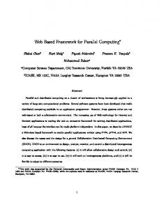
2.2 TLD in CUDA In [3], the authors study the most time-intensive stages of TLD, and then present a parallel algorithm based on CUDA. Their research is mostly invested in the detection stage of TLD, which is the most time consuming part. The other two stages remain on the host side using only the CPU for the computation. In the detection stage, three parallel algorithms were implemented: Variance Filter, Ensemble Classifier, and Nearest Neighbor Classifier. They used CUDA techniques to harness numerous computing units of the GPU to work together. Those three algorithms use the same input data and provide unified output, minimizing the transfer latency to and from the GPU device when each instance is called. A detailed diagram is shown in Figure 2.1, showing the steps of the CUDA-TLD implementation and where each phase of TLD is allocated to the specified computing device, i.e. GPU or CPU.

8

Figure 2.1: CUDA-TLD block diagram All experiments accomplished in this research used OpenCV-2.4.1 and CUDA4.1. The hardware specification of their experiments as implemented on both the CPU and the GPU, a 3.3GHz Intel, and 1.8GHz GeForce GTX 550 Ti respectively. Three different sizes of data sets were used as video inputs with the following resolutions: 320x240, 352x288, and 640x480. Their results showed that the speedup of the algorithm reaches up to 2.59X compared to TLD on some kernels while keeping the same detection percentile. Additionally, for the VGA standard input size, the CUDA implementation exceeded 18 frames per second rate, while the original implementation remained under 9 frames per second as its fastest rate. In this work, the authors had only parallelized the detection phase of the TLD implementation by Arthurv [26] using CUDA, and their results are based on a small dataset with similar resolution videos, with an exception of a single VGA dataset. The

9

speedups were obtained through comparing the latencies between the GPU and the CPU implementations (specifications mentioned above). In our work, we tested the parallel framework on different devices using a wide range of scaled inputs. Also, we emphasize the flexibility and portability of the implementation.

2.3 Hybrid CPU-GPU implementation of TLD In [24], the authors provide a recent parallel implementation of TLD using the computational capability of GPUs and a premium multi-core CPU, utilizing CUDA for the GPU and OpenMP for the CPU. Their parallel implementation is synonymous to the implementation discussed in Section 2.2. They harness the multi-core CPU to accomplish the GPU unfriendly portions (i.e. when data transfer far exceeds the execution time). They used an Intel i7 4770K 3.5GHz, with 4 physical cores and a hyper-threading factor of 2; and for the GPU they used an Nvidia Tesla K40. For software development tools, they used CUDA 6.0, OpenCV 2.4.9, and OpenMP 2.0; all installed on Windows 7 x64 Operating System. For low resolution videos, they achieved significant speedup of some kernels, about 2.82X for low resolution videos and 10.25X for Full HD quality videos. This implementation is similar to that presented in Section 2.2, with additional speedup obtained through cutting-edge hardware components and multi-core CPU utilization, i.e. complete TLD modification to be compatible with the specified hardware. In our work, we separated the acceleration techniques to deeper observe the application behavior, since we are trying to build a global parallel framework that is not only for the TLD algorithm, but also for other object tracking methods.

10

2.4 Motion tracking on Multi GPUs In [4], they present a methodology for optical flow motion tracking using the Lucas-Kanade algorithm. It is later made to work with the Harris corner detector and thereby may do sparse tracking, i.e. tracking of the important pixels only, which significantly lowers the processing burden of the method. Also, both parts of the algorithm, i.e. corner selection and tracking, are carried out on the GPU and as a result, the software is extremely fast, permitting real-time motion tracking on videos in Full HD or even 4K format. The implementation used OpenCV for video preprocessing and CUDA interface for GPU implementation of Lucas Kanade. The experiments were conducted on a machine equipped with: 2.33 GHz Intel Core 2 Quad Q8200, GTX 580 NVIDIA GeForce GPU with 1.5GB of RAM, and 8GB main memory. Figure 2.2 shows how Lukas Kanade implementation is achieved on the GPU. The CPU is only responsible for video preprocessing (extracting raw frames from a compressed video), while the GPU accomplishes the whole tracking process, which can be summarized in 8 subsequent steps: edge detection (or corner detection), building pyramidal images, pixel matching, gradient computation, temporal derivatives, optical flow computation, estimation correction (by matching with previous pyramidal image), and displaying output using OpenGL visualization as described in [4]. The research presented in [4] provides a parallel implementation of LK using GPU only, and the output is shown directly on the screen using OpenGL support of the GPU (i.e. results sink at the GPU and never return to the host). These results from the literature provided guidance for parallelization of the tracking phase of the TLD

11

algorithm. We leveraged their implementation to accelerate the tracking phase of our parallel framework with the ability of reviewing results at the host. We have not utilized muli-GPUs in this thesis research, but list it as future work.

Figure 2.2: Lucas-Kanade algorithm implementation on GPU [4]

12

2.5 Motion tracking using Deep Learning In [5], a totally different approach is utilized. The authors designed two-layer networks trained using either supervised or unsupervised learning techniques. The networks, integrated with a radial basis function classifier, are able to track objects based on a single example. They tested the networks tracking performance on the TLD dataset, one of the most intensive sets of tracking tasks and real-time tracking is achieved in 0.074 seconds per frame for 320x240 pixel image on a 2-core 2.7GHz Intel i7 laptop. The significant contribution from this approach is the ability to harness heterogeneous computing to implement such methods to obtain better results, especially when conventional computing produces limited results as presented earlier. Figure 2.3 shows successive images from a video is being processed to obtain the output.

Figure 2.3: Tracking approach with Deep Neural Network [5]

13

The authors used two layers network to find the output confidence map. The process can be summarized as: first, the RGB input is sliced into small patches, and then the small patches are fed to the network for convolution vector computation, then Pooling process is applied to generate spatial invariance while forwarding only important features to the following layer. The confidence map consists of values associated with the patches locations in the RGB input. The best confidence value narrows down the object location.

2.6 Summary In this chapter, different implementations of motion tracking applications are presented. The implementations are organized by the relevancy of the work to our scope. We discussed the differences of our model with other author works. The next chapter provides technical background for the TLD algorithm and the tools used in this research.

14

CHAPTER 3 BACKGROUND Based on the related work presented earlier, the next step is to carry out our own methodology, which is synonymous with a heterogeneous solution. Before introducing the methodology, concise highlights on the algorithm and the tools used for accomplishing this research is necessary. This chapter elaborates on the tools and techniques used in this thesis through four main sections. The first section discusses the mechanisms of the OpenCL environment, and how it is useful to our implementation. The second section is a “compare and contrast” illustration between OpenCL and CUDA platforms, with a brief reasoning of why we chose OpenCL and not CUDA. The third section introduces the OpenMP API as parallel environment for multi-core CPUs. Lastly, the fourth section describes the whole structure of the TLD algorithm emphasizing the parts we implement in our model.

3.1 OpenCL Environment Accelerated Parallel Processing offered from different vendors utilize the tremendous processing power of GPUs for high-performance and data-parallel computing in a wide range of applications. As an example, the AMD Accelerated Parallel Processing system includes a software stack, AMD GPUs, and AMD multi-core CPUs. Figure 3.1a illustrates the AMD Accelerated Parallel Processing Software Ecosystem and where the OpenCL runtime environment is located [11]. As shown in Figure 3.1b, OpenCL maps the total number of work-items, which are the hardware units that execute the kernel, to

15

be launched onto an N-dimensional grid (ND-Range). The programmer can decide how to specify these items into groups. In AMD GPUs, it executes on wavefronts (collections of work-items run simultaneously); there are multiple wavefronts in each work-group.

(a) (b) Figure 3.1: OpenCL runtime in AMD GPU (a) AMD Accelerated Parallel Processing Software Ecosystem, (b) Work-Item Grouping into Work-Groups and Wavefronts [11] In fact, there is an intermediate step for scheduling the work-items to run on a parallel computing device by specifying how many wavefronts are in a single workgroup. This leads to a customizable configuration that attains maximum parallelization. In our implementation, we used different criteria for each kernel, such that in color space conversion, RGB to Gray, we used 1-dimensional range, while in the Sobel filter we used 2-dimensional range. OpenCL runtime can run on multi-core CPUs as well, as various CPU and GPU architectures, but have very different outcomes for a specific kernel. For example, computing the X and Y gradients of different image sizes using the OpenCL framework on a commodity laptop showed positive results on the GPU. However, for best results on the GPU, the image dimensions should be a power of 2 such as 512, 1024, 2048 and so

16

on, assuming the input data is an image. Then, the distribution of kernels on the GPU queues will be equally spaced, utilizing all work-items simultaneously. For a simple demonstration, Table 3.1 shows some optimistic results. Table 3.1: OpenCL Gradient computation on CPUs and GPUs Latency CPU Intel core i5 3230M GPU AMD Radeon Image size type quad (ms) HD7650M (ms) Program 0.191454 0.0773813 512X512 Compute 0.006218 0.0009236 Kernel Program 0.25854 0.0749347 1024X1024 Compute 0.024492 0.00356956 Kernel Program 1.98372 0.301274 10240X6400 Compute 1.7935 0.23652 Kernel Program 1.98372 0.43275 10240X10240 Compute 1.7935 0.330216 Kernel For a simple speedup we compare gradient calculation on the CPU and GPU of a mid-level laptop. We can see how the speedup is not significant smaller sizes, but as the data size increases to the big data domain, we record strong scaling of the program and really good speedup on the OpenCL implementation for GPU; despite both CPU and GPU running on the OpenCL platform. This program compatibility for CPUs and GPUs is an advantage because systems without GPUs can also run the code on a multi-core CPU in parallel and it will still be faster than a sequential implementation.

3.2 OpenCL vs. CUDA For the last few years, GPGPU programmers have the choice to select a GPU interface for their application development, which can be either CUDA or OpenCL. Both

17

can achieve high performance computing and both can access lower levels of hardware [12]. In [13], the authors’ implementation of “the EMRI Teukolsky Code” on low-level parallelization using both OpenCL and CUDA showed equivalent performance. According to Kyle Spafford [12], at Oak Ridge National Lab (ORNL) from the Future Technology Group, their benchmarking of OpenCL and CUDA exhibited comparable results for both. Also AccelerEyes [14], a GPU Software Company, agrees with these conclusions. Therefore, understanding which interface to utilize depends on the nature of the application and the device type one is using; considering CUDA works only on NVIDIA based GPGPUs, while OpenCL can work on many different products. To bolster this assumption, the following subsections provide technical details that subsequently clarify the decision.

3.2.1 CUDA as GPU interface NVIDIA made the CUDA framework available in 2007 [15], since then it has assisted programmers in accessing lower levels of GPU hardware components by using C/C++ synonymous coding. With the introduction of CUDA, GPUs have become one of the most popular choices of accelerating technology in HPC. In [16], they used a Quantum Monte Carlo application as a comparison subject between CUDA and OpenCL. Their results showed better performance when using CUDA due to the fact that transferring data to and from the GPU is faster. Also, they found that CUDA’s Kernel execution is faster, although implementation codes are identical. In [17], they worked more thoroughly by performing extensive analysis of

18

selecting 16 benchmarks encompassing synthetic and real-world applications. Their results convey 30% better performance using CUDA than OpenCL. However, their conclusion involved the fact that some of the comparison guidelines lack fairness. This led them to perform more potential analysis of two applications with fair comparison, and the later exhibited similar performance. One more fact about CUDA that significantly makes it more preferable among GPU programmers is the availability of a proprietary tightly coupled CUDA library, various debugging and performance analysis tools, and rich technical support.

3.2.2 OpenCL as a parallel interface OpenCL first introduced by the KHRONOS Group in 2008 [18], a year after CUDA’s first proprietary development library was announced. Currently, OpenCL can be executed on CPUs, GPUs, DSPs, FPGAs, and other hardware. Its portability and open source standard makes it more promising than CUDA for future parallel programming, especially with the availability of multi-core CPUs in servers and embedded architectures. In contrast to CUDA [19], OpenCL’s synchronization feature is more flexible, (i.e. queued actions, like memory transfer or kernel execution, can be preempted to allow other operations to finish first). For C++ programmers, OpenCL spares object oriented programming bindings, while CUDA has a more restricted C API. And lastly, OpenCL can use function pointers as in CPUs in its CL_Command_Queues, but CUDA does not have this feature. Other minor differences found in [19], which does not reflect much to the scope of this thesis.

19

Besides the points mentioned above, the main reasons for selecting OpenCL and not CUDA were: first, OpenCL is more heterogeneous environment friendly than CUDA; second, although experiments show CUDA performs better in most applications, realtime applications are required to run on more generic devices, (i.e. not only heavy duty workstations but also embedded devices); third, the application we are pursuing is already implemented on CUDA, this gives us the opportunity to compare the performance of an OpenCL implementation to the similar implementations in the literature.

3.3 OpenMP API OpenMP is a portable interface for programming and stands for Open MultiProcessing. At its earlier stages around 1997, its developers aimed to build a unified model of coding to support shared memory systems [25]. Currently, it is supported by many vendors and compilers, and it is specifically used to harness multi-core processors through providing shared memory management among many processing units. In general, the availability of multi-core processors nowadays across almost all devices we use daily forces us to utilize tools that provide maximum use of resources and to migrate the conventional programming technique to the next level. In this thesis, we use OpenMP for performance analysis and result comparison of single core versus many cores depending on the available hardware specifications. Additionally, the OpenMP API is used to accelerate some code portions to provide maximum acceleration for the overall application but it remains optional since the acceleration depends on the hardware used.

20

3.4 TLD Application Long-term tracking has been very popular in real-time applications such as surveillance, cameras, warfare, etc. but highly scalable implementations are not common. For the application to be widely applicable, a scalable approach is needed. Conventional implementations use large data centers to support multiple video input infrastructure. For example, if there are thousands of surveillance cameras and the former implementation is used, there will be a significant performance bottleneck for tracking a specific object within all video streams. This section explores the algorithms that are essential for largescale TLD implementation.

3.4.1 Tracking There are many methods available for object tracking, but the one that is used in TLD is called Lucas and Kanade [20]. This method is very effective for tracking features that lay on non-homogeneous regions of an image, otherwise the feature would be difficult to track. To select good features within an interested object, preprocessing of the first image is required. However, since the object position is known by the bounding box (BB), a term used to define the boundary of an object in an image usually by a rectangular shape, as it is given in the first image, the later step is not necessary. Instead of finding good features, equally distributed points in the initial box are positioned as initial features [6]. Later, two techniques will be used [22], normalized cross correlation (NCC) and forward-backward (FB) error, and it will overcome mispositioned initial feature points. Figure 3.2 illustrates how erroneous features are removed in the second frame,

21

Figure 3.2: LK feature points: Frame (t): features initialization, frame (t+1): good features stabilization [22] The tracking process is recursive, (i.e. the new features position are inputs of the next tracking process). The Lucas and Kanade tracking method is based on three premises: brightness constancy, temporal persistence, and spatial coherence [6, 23]. The mathematical formulas are discussed later in Chapter 5. The two techniques mentioned earlier, FB and NCC, are corrective criteria for feature points and image patches (bounding box parts) respectively of two consecutive frames. The forward-backward error is basically a combination of the Euclidean distances between a feature point and its new calculated position, and the distance between the new location and its original shadowed point. Hence, the tracking process is implemented twice for computing the error between the two distances because the moving object points should have the same distance magnitude to keep the feature point validity. In [22], it chooses median FB distance as a point keeping strategy, (i.e. points with distance more than FB median will be removed from the feature set). The NCC technique instead calculates the brightness correlation between the old image patch and its new patch location. NCC uses a single value for each patch. Again, it takes NCC median as a threshold if the new image location represents the original object. 22

To avoid any erratic tracking, they set β FB as a default threshold for FB distance, (i.e. FB median value more than predefined threshold refers to stop tracking).

3.4.2 Detection In the previous section, we explained the tracker operation, but what will happen if the tracker loses the object? A simple way to find the object is to apply exhaustive search, looking for the object through the whole image. However, scanning the whole image requires considerable amount of time. Therefore, in [2] they used three techniques to reduce the search time. These techniques basically disregard image regions where the probability of object existence is minimal. Furthermore, the search operation will be more cumbersome if several versions of the object are obtained from the learning stage (discussed later). To clarify the whole detection process, we summarize the whole operation in two steps [2]: 1. Scanning Sub-Windows: The input to the detection stage is the video frame plus positive image patches of the object (obtained from first frame and learning stage). Based on the size of the object, the number of scanning sub-windows is calculated, which may range from 50,000 to 200,000 for VGA video resolution (640X480) [6]. Additional image preprocessing may involve alterations to the image patches such as resizing, scaling, stepping, etc. 2. Cascaded Classifier: In this step, sub-window patches are classified into two categories: accepted or rejected. To speed up the classification, the classifier is divided into three sequential stages, where each decides whether the image patch

23

can be rejected before forwarding it to the next stage [2]. These stages are: patch variance, ensemble classifier, and nearest neighbor classifier.

3.4.3 Learning This phase helps the detector locate the object more profoundly through negative and positive expert templates. The learning stage can be summarized as three main components [2]: 1. Initialization: The training process starts as early as the first frame. First, the initial object box is taken plus the closest scanning sub-windows that includes the object to a certain extent--which can be named as positive examples. Second, for each positive example, multiple wrapped versions are spawned based on random uniform distribution parameters like shifting, scaling, and in-plane rotation. Then additive Gaussian noise is applied for each version. In [2], the authors used 10 positive examples closest to the object and 20 wrapped versions for each one, resulting total of 200 positive patches. Third, for negative examples, negative patches are extracted around the initial box, and wrapped versions are not necessary for negative examples. 2. Positive expert: The job of this component is to update the positive examples with new object trajectory, size and brightness. How new positive patches are obtained is a sophisticated decision and depends on confidence parameters. In short, the tracker and the detector phases work in tandem, the tracker updates the location, and the detector compares the object with the positive patches. Any small change will trigger a middle phase, called an integrator, to produce new

24

positive examples and wrapped versions as in the initialization process. In this time, fewer positive patches are generated for the sake of efficiency. 3. Negative expert: The job of this component is to help the detector avoid background clutter, assuming that the object can be found in one location. Negative patches are updated when new positive patches are generated. In [2], a patch that overlaps the object 20% or less is considered negative examples. In this section, some image processing details are skipped for the sake of simplicity. Furthermore, some TLD parameters are flexible and can be changed depending on how much efficiency and accuracy is required.

3.5 Summary In this chapter, the technical background needed for implementation is presented for the terms that are mentioned in the previous chapters. The next chapter provides deep analysis for our model including more technical details within the scope of this thesis.

25

CHAPTER 4 ANALYSIS This chapter presents the analysis of two implementations available in the literature. It shows the timing behavior of the TLD application, and it studies the affect of input size and how it meets the thesis expectations. We thoroughly searched the application for components that can be executed in the OpenCL environment without putting a burden on the overall implementation. Furthermore, it explores and analyzes the timing measures of TLD application phases and algorithms. We select two TLD implementations: MOTLD and OpenTLD, provided by [9] and [26] respectively. The reasons for choosing MOTLD include: first, the implementation is new and fast; second, it does not depend on third party software, unlike the original implementation of TLD that requires software packages such as Matlab, OpenCV, Microsoft Visual Studio, etc.; third, it is customizable and well documented; forth, it runs on various Operating Systems like Microsoft Windows and Linux, (This is important for the fact that we faced technical compatibility issues in compiling some GPGPUs drivers on some Operating Systems due to the lack of vendor support); and last but not least, it has a multi-object tracking feature, which facilitates the stressful performance tests. The second TLD implementation presented in [26], has been used by the literature for parallel implementations. This implementation offers the best opportunity for results comparisons. However, this implementation is based on OpenCV, which has its pros and cons. The plus side of this implementation is having the phases built in separate modules, which facilitates in the insertion of parallel kernels without affecting other modules, and

26

collection of timing behavior for each phase. The negative side comprises of being dependent on third party libraries, which are tightly coupled and difficult to modify. 4.1 TLD Latency Analysis As discussed earlier in Chapter 3, TLD has three main phases: tracking, learning and detection. The detection phase is always on, with each input frame, while the tracking can be switched off when the object gets out of the image boundary or becomes untraceable. The learning phase depends on object trajectory change, so it is difficult to anticipate whether it is going to be on or off. To inspect more about the timing models of these phases, stress analysis is applied to the implementation in [9] and [26] using several video inputs obtained from the datasets available in [27] that have various dimensions and frame counts. Figure 4.1 shows frame samples of the tested videos. The first video sample in the figure (top left) pictures a pedestrian walking in a street with an unstable (unsteady) camera, the second (top right) plots a fast moving object, the third sample (bottom left) represents a jumping subject with the ability to track his face, and the last one (bottom right) ensures the application can track a moving subject with various brightness level (from dark to bright). Starting with the implementation in [9], Table 4.1shows the average time spent by each phase per frame as a total of four different inputs. As we can see, more than 50% of the computation time spent per frame is consumed by the detection phase for all inputs, followed by the tracking phase. The nn column in the table is the last filtering step of the detection and it is responsible for the final patch classification. Despite the fact that nn

27

has a small period proportional to the detection time, its value may escalate depending on algorithm parameters.

pedestrian.jpg

motocross.jpg

jumping.jpg

david.jpg

Figure 4.1: Frame samples of the tested videos taken from [27] For more clarification Figure 4.2 plots the timing bins of the values analyzed in Table 4.1. The results in Figure 4.2 and Table 4.1 quantify the sequential execution of the TLD application excluding any sort of acceleration. As in [3] and [24], our analyses ascertain that the most intensive computation occurs in the detection phase, where the whole filtering process takes place. Therefore, the majority of kernels are designed to reduce this phase. More details are provided in Chapter 5.

28

Table 4.1: Latency analysis for each TLD phase of MOTLD Average latency per frame (ms) Video sample david 320x240 (761 frame) jumping 352x288 (313 frame) motocross 470x210 (100 frame) pedestrian 320x240 (140 frame) Average Latency

Tracker

Detector

nn

Learner

Total

11.65263

65.2855

0.4855263

0.56842

77.99211

15.06731

66.3846

0.4519230

1.073718

82.9775

13.84848

23.808

0.0606060

0.939394

38.65656

10.58993

31.8849

0.122302

0.43165

43.0287

15.06731

66.3846

0.4519230

1.073718

82.9775

Figure 4.2: Timing diagram for TLD phases of MOTLD These results do not show the application behavior as the when input size is scaled to a higher dimension. Most of the videos in the dataset provided by the author in

29

[27] have particularly small sizes. Also the outcomes from each phase varies from one video to another because the tracked object is not contiguous in all frames, which may affect the aggregate latency, and as a result different videos produce different timing behavior. Therefore, the above analysis is insufficient to support a scalable parallel framework; instead the application was tested with a range of scaled video inputs starting as low as the QVGA standard up to the 4K high definition standard, with all having the same tracking results. Table 4.2 shows our results and the scalable analysis of the application regarding the average time spent in each phase for each input size. The graph shown in Figure 4.3 illustrates each phase latency behavior against the input size increment. Table 4.2: TLD analysis against input size of MOTLD Average frame phase latency in (ms) Input size

tracker

detector

nn

learner

sum

320x240

18.0000

4.5000

0.0000

0.0000

22.5000

640x480

17.1683

53.6238

0.6733

2.1485

73.6139

720x480

17.2376

40.4653

0.4554

2.7228

60.8812

1280x720

28.0891

103.0990

0.7624

5.7723

137.7228

1440x1080

38.1584

177.3960

0.6238

8.7030

224.8812

1920x1080

50.9307

268.4653

0.7228

11.2673

331.3861

3840x2180

181.8416

1004.2178

1.3168

35.6931

1223.0693

What we can observe from Figure 4.3 is that the processing time scales linearly as the number of pixels increases. Further, the total time required for the last two input sizes is not tolerable for a real-time application.

30

Figure 4.3: TLD phases behavior against input size of MOTLD The second TLD implementation, which is available in [26], is more modular and performs better in terms of object tracking but with the cost of frame latency. The implementation method is more synonymous with the first implementation by the author Kalal [2]. The previous tests are repeated for this implementation and the results are shown in Tables 4.3 and 4.4 with the corresponding graph illustrations plotted in Figures 4.4 and 4.5 respectively. Table 4.3: Latency analysis for each TLD phase of OpenTLD Average latency per frame (ms) Video Input

Tracker

Detector

Learner

Total

david

6.226404011

13.03367479

4.564010929

20.45666046

jumping

5.983371795

31.55411218

0.1658996764

37.70178846

pedestrian

5.060863309

47.86902158

1.454297101

54.37371942

motocross

7.000970588

12.20951961

0.0653627451

19.27585294

Average

6.067902426

26.16658204

1.562392613

32.95200532

31

Table 4.4: TLD analysis against input size of OpenTLD Average frame phase latency in (ms) Input Size

Tracker

Detector

Learner

Total

320x240

6.376748954

56.95876569

2.036778243

65.37229289

640x480

8.585723849

37.73978661

0.8032301255

47.12874059

720x480

9.254376569

44.21420921

0.9001924686

54.36877824

1280x720

11.51897908

79.76250628

2.702200837

93.98368619

1440x1080

17.3531841

104.0465397

3.860214286

125.2437866

1920x1080

21.74756485

135.1211255

4.177096234

161.0457866

3840x2160

73.91930962

175.2103598

3.703691983

252.8023682

Figure 4.4: TLD phases timing analysis for OpenTLD From Figures 4.4 and 4.5, we see that the results only differ from MOTLD in the average latency. The measured latency for the OpenTLD does not include some intermediate operations (the total frame time is higher than what is shown in Tables 4.3 and 4.4) due to the common data tables and functions used by all phases. Conversely, in MOTLD all operations for each phase are implemented in separate modules.

32

Figure 4.5: TLD phases’ behavior against input size of OpenTLD The detection phase is typically a major bottleneck compared to the other phases as the input size increases. Also, we can see that the detection phase at 320x240 resolution is defying the curve due to the low quality of the image (down sampled from a higher resolution video). Down sampling leaves the detector open to more possibilities and an increased number of bounding boxes inside each frame, which then deteriorates the detector operation. After investigation of each phase, further analysis is required at the algorithm level, which is discussed in next section.

4.2 TLD Algorithm Analysis This section investigates the algorithms used in TLD and implementable on a parallel computing device. As introduced earlier not all algorithms can produce positive results if implemented on a parallel device, at least for real-time applications. Even cases where the most parallelizable components are implemented, slowdown in the overall

33

application performance can occur. The rest of this section is organized by phase with the associated algorithms.

4.2.1 Tracking algorithms Tracking comprises of five steps: calculating the optical flow of the identified feature points (produced in frame initialization), backward optical flow calculation for newly located feature points, forward-backward (FB) error calculation between the original feature points with the ones calculated in the second step, normal crosscorrelation calculation for image patches associated around the feature points, and lastly filtering points based on the FB error values computed earlier. The first two steps use the same pyramidal Lucas-Kanade method (PLK) algorithm with reverse parameters. So if we get a significant improvement in a parallel (PLK) implementation it benefits both. The third step poses only subtraction between two points, which can be parallelized but it will be inefficient due to the limited number of points. The fourth step can be generalized as a template matching between two image patches, which also can be easily parallelized especially when using large patch sizes. The last step has the same deficit as step three. Deep latency analysis is applied to the tracking phase as shown in Table 4.5 and depicted in Figure 4.6. Table 4.5: Tracking algorithms latency for different inputs (ms) Video input LK1 LK2 FB_error NCC motocross

2.343779

2.308470

0.00269

2.23395

pedestrian

1.83004

1.9404

0.0028

2.50362

jumping

1.94262

1.99350

0.002531

2.3665

david

1.41245

1.45533

0.002417

2.13715

34

Figure 4.6: Tracking algorithms deep analyses Table 4.5 and Figure 4.6 present the latency differences of the first four steps in the tracking stage (the latency of the fifth step is negligible). LK1 and LK2 represent the two optical flow calculations. From the measurements, we see that only three steps are worthy to parallelize, which are represented by the two algorithms PLK and NCC.

4.2.2 Detection algorithms This section explores the main bottleneck points that make the detection phase the most time consuming phase. This phase includes many steps and levels, and they are executed in a sequential manner. Based on the size of the frame and the object, the number of candidate bounding boxes (BBs) is generated (can exceed 300,000 BBs for a VGA video input). From these BBs, only the top hundred or less are selected based on a similarity confidence to the BB from the previous frame. The whole process can be

35

summarized as three level filtering: variance filter, ensemble classifier, and template matching. For variance filtering, two main parameters should be calculated from the BBs patch before making a filtering decision: BB’s Sum Area (SA) and Square Sum Area (SSA). After passing this level of filtering, the BB is processed for fern features that are used to compute a confidence value, this value should be greater than a predetermined threshold to enable the BB to pass to the next level. For better confidence determination, the BB should be blurred with a Gaussian filter. Detections from the second level are assembled in a data structure for further processing. If the number of confident BBs is higher than a default parameter, (typically around 100) the best BBs can be extracted by their highest confidence values. The reason for this reduction is to forward the fewest number of BBs as possible to the next level, which is a more computationally expensive level. The last step of detection process is to compare the remaining BBs with the original BB (the one in the previous frame) for full pattern match, and then the one with highest similarity can be selected as the best BB for the current frame. This BB is forwarded to the tracker if the object has been tracked and to the learner if some object features have been changed to what is available in the learner’s repository. Major speedup can be exploited in the first and second level, since the number of BBs is significantly high. As the frame dimension increases the number of BBs in a frame increases as well. A basic method to estimate the number of BBs that a single frame has is to apply the following equation [6], 𝑁𝑜. 𝑜𝑓 𝐵𝐵𝑠 = (𝑊 − 𝐵𝐵𝑤𝑖𝑑𝑡ℎ) ∗ (𝐻 − 𝐵𝐵ℎ𝑒𝑖𝑔ℎ𝑡) 36

(Eq. 4.1)

where (W, H) are width and height of the frame respectively, and (BBwidth, BBheight) are bounding box dimensions. Timing analysis for detection algorithms is not analogous to the tracking phase because of the nested behavior of the BB filtration process. The best way to present a good timing estimation is by counting the number of BBs in each step. Table 4.6 shows BBs’ count for each step of the detection stage for a selection of video samples. We see that the total number of BBs depends on the input size. Whereas, the variance filtered BB’s depends on two factors: input size and video background texture. The remaining BBs after the Fern Classifier step does not depend on the input size or on the background texture, but rather on the object texture. In Figure 4.5 we notice an odd TLD latency startup when processing the 320x240 video, it consumes more time than 640x480 video. The reason is obvious when we check the remaining BBs at the end of the detection stage. Table 4.6 Detection stage latency analysis through number of BBs Video name

Number of BBs Total BBs

Variance Filter output

Fern Classifier output

average

median

average

median

average

median

motocross

143642

143642

9544

8963

15

10

pedestrian

69310

69310

28103

28571

11

11

jumping

98433

98433

45063

45299

10

9

david

58901

58901

54982

56033

1

1

320x240

66763

66763

10351

10637

108

107

640x480

258044

258044

24255

23640

64

64

720x480

285432

285432

28161

27501

64

62

1920x1280

2289439

2289439

109310

101196

18

18

37

4.2.3 Learning algorithms Learning algorithms update positive examples whenever a newly detected and tracked BB has different characteristics than what exist in the training repository. Timing analysis for both implementations shows that the learning step is not a significant bottleneck for the whole application, even when using a large scale input. For this reason, we kept this phase out of the parallel framework.

4.2.4 Other algorithms There are some preprocessing steps for the frames prior to forwarding to the TLD phases. Some of these steps can be parallelized as well, but they are not very effective in terms of efficiency. These steps include some image processing and preparation such as converting color components to gray level, resizing images, rotating images, etc.

4.2.5 Analysis conclusion As a conclusion from the observation and analysis the following conclusions are offered: 1. The behavior of the application is not the same for each video input and object size. 2. Input scaling keeps the behavior unchanged as long as the object can be tracked. 3. The Detection phase is the major bottleneck for all types of inputs and parameter changes. 4. The Tracking phase could be a bottleneck as input scale increases. 5. The Learning phase remains in the acceptable delay zone for most video inputs.

38

6. There are marginal differences in timing between the two implementations because the first implementation (MOTLD) is designed for speedup rather than tracking efficiency, while the second (OpenTLD) prefers tracking efficiency over latency.

4.3 Summary In this chapter, we analyzed the TLD application using two different implementations available in [9] and [26]. This chapter investigated the timing behavior of each phase of the algorithm and pinpointed the modules where the majority of latency is incurred. The next chapter provides the main methodology for designing a parallel framework for long-term tracking with the use of various implementation scenarios.

39

CHAPTER 5 DESIGN AND IMPLEMENTATION After deep analysis of the algorithm on our selected hardware platforms using two implementations available in the literature, this chapter presents the core components of this thesis. It shows the mathematical models of TLD algorithms, and it studies the affect of partial modifications. TLD is not a parallel friendly algorithm. Most components can run better sequentially. We thoroughly searched the algorithm for components that can be executed on the OpenCL environment without putting a burden on the overall implementation performance. Our approach attempts to mitigate this bottleneck through a better computational environment, which can use different hardware components to achieve the same performance with much less cost. This chapter is divided into three main sections. The first section introduces the steps of deploying parallel implementation of an algorithm, and lists the design methodology we followed in this thesis with a simple example of creating a parallel kernel using OpenCL. The second section derives the design model of the TLD parallel implementation; by implementing each kernel individually then combining them into a unified model. Section three provides various implementation scenarios for testing the model. The last section summarizes this chapter.

5.1 Parallel Framework Methodology Many tools, IDEs, and programming techniques have been developed and introduced recently to facilitate and support widespread use of parallel systems. In [15],

40

they classify parallel coding as an iterative process of software development that can be generalized through these steps: 1. Locate the code section that has unutilized parallelism in the original source code. 2. Select a fitting programming technique to achieve parallel acceleration. 3. Apply and augment the parallelization inside the original source code. 4. Validate the output. 5. Justify the performance of the application. These steps may be repeated to other sections of the source code till maximum parallelization is employed. Figure 5.1 depicts a simple diagram for the iterative parallel coding process.

Figure 5.1: Parallel coding as iterative process

41

Based on the iterative model, we derived the mechanism for parallel TLD implementation summarized by the following: 1. Design kernels for different inherent algorithms utilized by TLD. 2. Stress and analyze the performance of these kernels on both CPU and GPU. 3. Locate the delay points and critical paths with regards to data and resource availability (this is to ensure real-time efficiency within an acceptable boundary). 4. Check the global speedup by implementing all the kernels within the sequential program on both CPU and GPU. 5. Trigger parallel kernels whenever their efficiency is acceptable. 6. Finalize with a self-adapting parallel framework that achieves high scalability and meets the real-world demands. The presented steps can be considered a rule-of-thumb and can be implemented on other algorithms. As an example of a single kernel parallelization, the following subsection describes the whole process of color space conversion from RGB to Gray, essential for TLD, using a simple kernel.

5.1.1 Example: RGB to Grey level Conversion Kernel in OpenCL One of the steps essential for the TLD algorithm is converting the input from the standard RGB color format to gray scale, because the TLD algorithm is based on gradient computation, which requires gray scale input. After implementing this step serially we investigate penalization of this pixel-based compute intensive section. We wrote an OpenCL kernel to bring massive parallel operation to this unit. The RGB-to-Gray conversion is based on taking the Red, Green and Blue intensity components of the 42

colored image and taking the average of their sum respectively. This average value is stored for the pixel in the converted gray scale image. The Red, Green and Blue pixels are passed as float values to the compute kernel and the gray scale level is also stored as float. The following list shows the steps followed to run the OpenCL kernel: 1. Declare the OpenCL buffers, which are signals and values to be used as arguments for calling the buffer. 2. Choose the device to be used by the OpenCL directive GET_DEVICE_ID_CPU or GET_DEVICE_ID_GPU, depending on the target device for the kernel. 3. Define the wavefront design by assigning values to global and local work groups IDs. 4. Create the buffers for kernel inputs and a buffer for the kernel output. 5. The kernel is built as a program with the next command, and then the kernel is executed with the input buffers loaded into device memory and the output buffers downloaded to the host, after all the process streams finish computing. 6. Assign the output date to the output buffer and write the data to an output file. This methodology for creating, building and executing is also used for the other kernels. The above kernel implementation is inefficient for an accelerator device because the kernel itself is computationally simple, therefore implementing it on the host is more reasonable and efficient yet the decision ultimately depends on the CPU specifications and the task characteristics.

43

5.2 Parallel Framework Design This section provides a detailed discussion of the algorithms that can be accelerated using available devices that support the OpenCL API. Based on the analysis and timing diagrams presented in the previous chapter, algorithms are selected from the TLD implementations in [9] and [26]. Each algorithm is parallelized, tested and executed in a standalone situation for the sake of recording results and comparing efficiency. Timing diagrams for each parallel kernel implementation are recorded and compared with the sequential implementation across scaled inputs. Parallel implementations for long-term object tracking can be affected by many factors: algorithms’ timing behavior, input video classification and dimensions, hardware specification, available APIs, application parameters and preferred precision, and other application designer preferences like timing constraints and power consumption. Thus, developing a single fixed platform might be inappropriate for the wide spectrum of video inputs. The final application includes all parallel modules as well as the sequential ones. Decisions are made whether to use sequential or parallel modules depending on the learning curve of the application efficiency when it executes the first time; giving the system the opportunity to calibrate itself to the best performance curve. It is unreliable to design a fixed system through testing it on a limited number of inputs. Instead, using our model will ensure that long-term tracking applications will adapt and produce the best performance based on the application’s response for each kernel. Moreover, it can also sustain hardware changes if hardware devices are upgraded over time.

44

The remainder of this section is organized as two subsections. In the first subsection, each algorithm is introduced with a mechanism of parallelization. While in the second subsection, the top parallel framework is built using all kernels combined with an explanation of their operations.

5.2.1 Parallel algorithms design The kernels that are designed in this chapter are based on the studies in previous chapter. Each kernel design is contingent on the analysis from the original application. Some kernels use the same design techniques, so for the sake of brevity, redundant designs are referenced to a shared category. Furthermore, this subsection includes the mathematical models for each kernel plus the corresponding approach that extracts the inherent parallelism. The kernel designs are arranged beginning with the most general to the more specific.

5.2.1.1 Reduction based kernels The reduction technique that reduces a large vector into a smaller vector or single scalar, usually done by separating the vector into equally sized chunks, each chunk is executed on a distinct computing unit simultaneously (multi-core CPUs or streaming processors in GPUs) [28]. Reduction is useful when a similar operation is performed on each data items of a large dataset Examples of reduction kernels are Sum, Square Sum, Average, Minimum, Maximum, etc. Figure 5.2 depicts reduction process of having the sum of 8 numbers using three level trees.

45

Figure 5.2: Three level Sum Reduction Tree [28] Reduction can be implemented in many strategies, the simple ones use mathematical properties: associativity and commutativity. To implement sum reduction on GPUs using OpenCL, certain steps should be followed [29]: 1. Using the associative property, divide the vector into small sub-vectors. e.g. (a+b+c+d+e+f….) will be ((a+b) + (c+d) + (e+f).....). Each work-group will be responsible for a sub-vector. 2. Each sub-vector will have its own reduction tree, each sub-vector will be reduced independently and in parallel. 3. If each sub-vector can be held in a local memory, then each element can be assigned to a work-item.

46

4. Performing reduction for each tree stage requires loading and storing of the branch results. This is why it is important to use local memory, so work-items can share results with work-groups. 5. The whole process can be summarized as a loop obtaining results from each stage plus setting barriers for memory updates. There are many limitations to using this strategy and each one can be solved with a specific technique: 1. Vector size consistency: make the number of work-items a power of 2 for each work-group, requiring the number of vector elements be consistent with the workitems, which can be solved by padding the necessary zeros to the vector to make it a power of 2. 2. SIMD structure: the above strategy can be more SIMD friendly if the commutativity property is used. To clarify, the difference between associativity and commutativity, Figure 5.3 (a-b) shows how SIMD utilization can be better achieved from commutative property. In commutative reduction, the blocks are contiguous and the allotted wavefronts for each work-group will be reduced, minimizing the execution time. 3. Vector size per work-group: when the vector size does not fit in a single workgroup, several methods can be employed: recursive multistage reduction, two-stage reduction, or reductions using atomics. All methods provide reduction scalability and are self-explanatory except for the atomic one, which is AMD API device specific, and more details can be found in [29].

47

(a)

(b) Figure 5.3: Reduction types: (a) Associative reduction (b) Commutative reduction [29] Kernels that are used in the TLD application and exploit parallel reduction are Sum, Average, Square Sum, and Image Integral. Some of these kernels may not appear explicitly but rather as a part of a larger kernel (e.g. Image Integral uses Sum and Square sum). These kernels are tested and analyzed in next chapter.

48

5.2.1.2 Window-based kernels Window-based kernels are popular in image processing due to the use of 2D window. Many image processing algorithms such as filtering, transforming, edge detection, etc. use small window convolutions across the entire image. This repetitive process can be easily implemented on parallel computing devices by mapping a computing unit with a corresponding memory addresses to perform the specified processing. However, memory buffers are logically 1-D vectors, so the windowing approach should be carefully implemented (careful memory management and addressing for each convolved window). Recent convolution implementations favor the use of 1-D kernel passed horizontally then vertically [30]. It has been shown that using the latter method increases efficiency. The two-pass method is considered an efficient convolution implementation as explained via a 3x3 example in [30]: 1. Suppose we have a pixel at location P(x,y) and 1-D horizontal kernel of H[a b c], the first horizontal pass will result in: h0 = p(x-1,y-1) * a + p(x,y-1) * b + p(x+1,y-1) *c

(Eq. 5.1)

h1 = p(x-1, y) * a + p(x,y) * b + p(x+1,y) *c

(Eq. 5.2)

h2 = p(x-1,y+1) * a + p(x,y+1) * b + p(x+1,y+1) *c

(Eq. 5.3)

2. The second pass (vertical) will reuse the above results directly to produce the final convolved pixel F(x,y) as in: F(x,y)= h0*a + h1*b + h2*c

(Eq. 5.4)

3. The efficiency come from the horizontal pass transpose of the output to columnwise instead of row-wise, and then the vertical pass work as row-wise without

49

modification of the with memory dimensions, since it is already transposed in the first pass. This method will also reduce the second pass computation leaving us with (3-horizontal and 1-vertical computation). 4. Furthermore, the next pixel will reuse h1 and h2, since they have already been computed for the previous pixel, reducing the total computation to (1-horizontal and 1-vertical). 5. In terms of memory bandwidth, this method will reduce nine-pixel fetch into sixpixel fetch but it requires two write operations, which yields eight R/W operations in total, while the 2D-implementation requires ten R/W operations (9 for read and 1 for write). Figure 5.4 depicts the entire two pass convolution. As a GPU device, memory operations are considered expensive, so reducing I/O operations can be a crucial benefit. Kernels in the window-based category includes: Sobel, Gradient, and Gaussian smooth filters.

Figure 5.4: Two pass convolution process [30]

50

5.2.1.3 Pixel based kernels Pixel based kernels include algorithms that usually depend on the pixel itself such as color space conversion, noise addition and removal, pixel comparison, etc. There is no general implementation of such kernels since each algorithm has its own computation method. Parallel implementation of such kernels follows a simple mathematical operation on each pixel or group of pixels. The output can be mapped to a vector, if it is a one-toone relationship, or to a scalar if it is many-to-one relationship. These kinds of kernels can be easily implemented on GPU devices due to the simplicity of the kernel structure (simple input/output mapping). Kernels that reside in this category in TLD are RGB-toGray conversion, Normalized Cross Correlation (NCC), and image down sampling or resizing.

5.2.1.4 Special purpose kernels These kinds of kernels can be composed of several sub-kernels of different categories, i.e. multiple kernels use the same device memory and work collaboratively, each using one of the above mentioned techniques to produce a multi-stage output. These kernels are the most complex because they require extra care for memory management, since all sub-kernels may access and change the same shared memory locations. The purpose of using such complex kernels is to exploit common data usage among different kernels, reducing the number of data transfers from host to device and vice versa. One example of a special purpose kernel found in our parallel framework is Parallel Pyramidal Lucas Kanade (PPLK).

51

5.2.2 Parallel framework design for long-term tracking The TLD method for object tracking has many steps and components. Some of the components are essential and some can be optional. For better results, all steps followed by the original author [2] should be implemented with suitable parameter settings. As explained in Section 5.1, we follow the same strategy for building a parallel implementation. Furthermore, some additions were applied to make the model flexible and highly portable. To describe the parallel implementation, first we show TLD components in a diagram, and then pinpoint the parts that can be replaced with efficient parallel kernels. A decision should be made whether the part should be replaced or remain unchanged based on a performance factor. Therefore, a new block should be added to the iterative parallel coding process, shown in Figure 5.1, which embodies the decision process and receives the feedback from the performance block while it is running. To provide further explanation, the next two sub-sections describe the usual data flow in the TLD algorithm and the necessary changes to ensure better parallel environment.

5.2.2.1 TLD data flow We introduced TLD as a long-term object tracking method and discussed the mechanisms it uses to track objects. Now we explain what actually happens when a sequence of images enters the system. Figure 5.5 shows the data flow for the implementation in [26]. As seen in the diagram, the system assumes continuous object

52

availability; otherwise some blocks will suspend processing until the object becomes tracked again. All blocks are dependent on each other, this precludes frame pipelining. One can say that some portions of the blocks have fixed inputs (as in the preprocessing stage, Gaussian filter, and others). Thus, there is a possibility to process frames in groups (multiplexing) while awaiting other blocks to finish processing, and then provide single preprocessed frames (de-multiplexing) whenever possible. However, this method is useful when processing offline videos (i.e. archives), and it is not applicable for real-time video processing scenarios. Further, it requires more memory units for storing and processing.

5.2.2.2 TLD parallel framework As shown in Figure 5.5, all blocks are depicted as separate modules (we do not show all components of TLD for the sake of simplicity), this facilitates understanding of parallel implementation mechanism. As provided in the previous section, the parallel kernel associated for TLD blocks are many, to simplify the whole operation, we separate each phase into a different section, skipping two stages: initialization stage since it runs one time only, and learning stage because of negligible processing time.

5.2.2.2.1 Preprocessing stage This stage varies from one implementation to another; it depends on the type of input to the system. As an example, if it is raw (uncompressed), meeting the required dimensions, and having gray level color space, then no preprocessing is required. Otherwise, any of the missing input requirements should be resolved.

53

Figure 5.5: TLD data flow In our implementation, we exploit two preprocessing stages: RGB-to-Gray conversion and input resizing. Figure 5.6 describes the parallel implementation for the 54

preprocessing stage. The cubing blocks represents parallel implementation, while the dotted arrows and borders indicate optional stages and blocks respectively. Hence, before input frames are forwarded to one of the processing blocks, a decision should be made whether to choose the parallel implementation or the sequential one. The block named “Performance factor” is updated through an external performance evaluator, which controls the triggering operation for all kernels. Lastly, it is possible for the frame to be processed by any combination of the preprocessed blocks depending on the input, performance factor, and requirements of the next stage.

Figure 5.6: Parallel implementation for preprocessing stage

55

5.2.2.2.2 Tracking stage The tracking stage comprises of three steps, two optical flow tracking functions and one template matching. The optical flow tracking used is called, “Pyramidal Lucas Kanade feature tracker” (PLK) [31]. Optical flow tracking determines the displacement between feature points located on the first frame and their new locations in the next frame within a moving picture. Let u = [u x u y ]T be the vector of feature points, and d = [d x d y ]T be the vector that represents the velocity of the image at location x, and v be the vector of new locations’ points, then, v=u+d

(Eq. 5.5)

the velocity of the optical flow can be measured using this general formula [31]; 𝑢𝑦 +𝑤𝑦 𝑢𝑥 +𝑤𝑥 ∑𝑦=𝑢 (𝐼(𝑥, 𝑦) − 𝐽(𝑥 + 𝑑𝑥 , 𝑦 + 𝑑𝑦 ))2 𝜖𝜖(𝑑) = 𝜖𝜖�𝑑𝑥 , 𝑑𝑦 � = ∑𝑥=𝑢 𝑥 −𝑤𝑥 𝑦 −𝑤𝑦

(Eq. 5.6)

where, 𝜖𝜖 is velocity residual function.

I, J are the first frame, next frame respectively, and w x , w y are the integration window dimensions (usually 2,3,4,5,6,7). Image pyramids can be computed in a recursive fashion with this equation [31]: 1

1

𝐼𝐿 (𝑥, 𝑦) = 𝐼𝐿−1 (2𝑥, 2𝑦) + (𝐼𝐿−1 (2𝑥 − 1, 2𝑦) + 𝐼𝐿−1 (2𝑥 + 1,2𝑦) + 𝐼𝐿−1 (2𝑥, 2𝑦 − 4 8 1) + 𝐼𝐿−1 (2𝑥, 2𝑦 + 1)) +

1 (𝐼 (2𝑥 16 𝐿−1

− 1, 2𝑦 − 1) + 𝐼𝐿−1 (2𝑥 + 1, 2𝑦 + 1) +

𝐼𝐿−1 (2𝑥 − 1, 2𝑦 + 1) + 𝐼𝐿−1 (2𝑥 + 1,2𝑦 + 1))

56

(Eq. 5.7)

where, I: original image (the highest image resolution, or level 0 pyramid), L: level of the pyramid, and x, y: pyramid image dimensions. To find the dimensions (x, y) of each pyramid level, we can use these two simple recursive formulas, 1

(Eq. 5.8)

1

(Eq. 5.9)

xL ⩽ 2(xL-1 + 1) yL ⩽ 2(yL-1 + 1)

The optical flow equation (5.6) is applied to all pyramid levels (TLD usually uses 5 levels) starting with the lowest level (lowest image resolution level), with the corresponding u vectors that can be identified using the following formula: uL = u/2L

(Eq. 5.10)

Next, the results of each pyramid are forwarded to the upper level as an initial guess for the new pixel location. The result of the overall computation can be expressed as: d = 2LdL + 2L-1dL-1 + 2L-2dL-2 +…. + 2L-mdL-m

(Eq. 5.11)

where m is the maximum number of levels. The second type of tracking algorithm is the template matching between two patches using Normalized Cross Correlation (NCC). NCC is a scalar that represents the correlation between two image patches (in TLD, it is usually 15x15 pixels) and it follows the following formula:

57

𝑁𝐶𝐶�𝑃𝑖 , 𝑃𝑗 � =

2

∑𝑥,𝑦�𝑃𝑖 (𝑥,𝑦)∙𝑃𝑗 (𝑥,𝑦)�

�∑𝑥,𝑦 𝑃𝑖 (𝑥,𝑦)2 ∙∑𝑥,𝑦 𝑃𝑗 (𝑥,𝑦)2

(Eq. 5.12)

where, pi, pj : first image patch and the next image patch respectively, and x, y : pixel coordinates within the image. After showing the mathematical models for the tracking stage, it is time to observe their parallel implementation in the parallel implementation. As explained earlier, the PLK kernel operates under the special purpose kernels, while the NCC resides in reduction based kernels. PLK is executed twice for each frame, which makes it an interesting algorithm to accelerate. The input of the tracking stage comprises of two preprocessed frames (frame t and frame t-1 ) and feature points propagated from the previous frame. Likewise, the output provides the new point locations. Based on these points, the detector will checkout the new BB location within a frame. What makes TLD tracking robust is the presence of extra checking steps for error correction. The second PLK pass and NCC ascertain the first pass of PLK is providing accurate results. The tracking stage data is shown in Figure 5.7. As in the preprocessing stage, the cubic blocks represent the parallel the implementation (block name has an extra P) and the dotted arrows indicate that the flow may not be the same for all frames. Hence, there is no need to check the second PLK performance since it resembles the first.

58

Figure 5.7: Tracking stage data flow

5.2.2.2.3 Detection stage This stage is the most time consuming one but the least complicated. The whole detection process comprises of filtering false BBs within a frame. The task of detection becomes more important when the object disappears (lost) from the frame. As we can see in TLD data flow diagram Figure 5.5, the detection phase has mainly three filtering stages. However, there are many in-between computations that dramatically slow down the filtration process. A naive implementation may follow this procedure: 1. The frame is scanned for all possible BBs that may have properties similar to the previous identified BB, if available; if not, then positive examples are used as indicators. The candidate BBs are stored in a data structure as the very first pixel

59

of the BB (top left corner) along with the width and height. This operation will produce hundreds of thousands of BBs. 2. In the first level filtration, BBs with homogenous regions are excluded (usually background texture). To do so, the variance of each BB is calculated, and then compared with a variance threshold for the filtering process. To calculate the variance of a BB, the following formula is used: Variance (p) = E(p2) - E2(p)

(Eq. 5.13)

where, p: represents the grey level vector of all pixels inside the corresponding BB, E: represents Mean value, and E2: represents Square Mean value. The variance threshold is not a fixed number. Likewise, its value can be obtained from Equation 5.13 from the very first BB (best BB). BBs with variances greater than or equal the threshold are forwarded to the next filtration step. Finally, this step approximately reduces the number of BBs by a factor of 10X (i.e. 300,000 BBs will be reduced to 30,000). 3. The second filtering process is the fern filter. This step involves pixel comparison between the original BB and the candidate BB. Not all pixels are compared; instead a few random pixel locations (ferns) are picked up from BBs to compute confidence values. Confidence values higher than a selected confidence threshold are passed to the next level. However, exact pixel location comparisons of moving objects produce values far from what it should be. For this reason, the frame is

60

applied to a blurring process through using big window size Gaussian filter (usually (9, 9), with a predefined sigma). The following formula is used to build a Gaussian kernel [32]:

where,

𝑔(𝑥, 𝑦) = 𝑐𝑒

−

(𝑥2 +𝑦2 ) 2𝜎2

(Eq. 5.14)

g(x,y) represents the 2D kernel component coordinates ((0,0) is the center of the kernel), c is the scaling factor, and

𝝈𝝈 is the Gaussian filter smoothing factor.

The resulting window is convolved with the frame to produce a smooth image. This process dramatically reduces the number of BBs to a few hundred. 4. The last filtering process constitutes a heavy computation for each remaining BB. Therefore, only the BBs with the top 100 confidence values are processed through this stage (pre-filtering). The NCC values are computed for the remaining BBs. Once again, the one having the lowest difference value from the original NCC is chosen as the next best BB. We have two unexploited heavy computational steps: variance filter and Gaussian image. For the first one, we can use two parallel integrations: integral sum, and integral square sum for the whole frame, and then when it comes to the sum area and sum square area, 4 lookup table fetches are needed for each then through using the following formula, both values can be computed:

61

Area Sum (AS) or Area Square sum (ASS) = (A+D) - (B+C)

(Eq. 5.15)

where, A: represents the top-left corner value of integral image, B: represents the top-right corner value of integral image, C: represents the bottom-left corner value of integral image, and D: represents the bottom-right corner value of integral image. We obtained the idea of parallel integral image technique from [33]. Figure 5.8 illustrates how integral images are useful in finding a BB area sum. The same methodology can be used for finding area square sum.

Figure 5.8: BB’s sum area from an integral image [21] For the Gaussian filter, we use a window-based kernel as described in the previous section. The parallel framework for detection stage is depicted in Figure 5.9. As described earlier, the cubic blocks indicate the parallel implementation components of the stage, and their usage depends on the pre-calculated performance factor. Also, as we can see, Area sum and Area square sum share the same input due to the usage of the similar kernels and memory operations.

62

The PNCC block is reused from the tracking stage since it is the same algorithm. Lastly, there are some in-between operations related to the TLD that we ignore due to their irrelevance in our parallel framework.

Figure 5.9: Parallel framework for detection stage

5.3 Implementation The entire implementation process can be as brief as applying the parallel design to specific computer hardware, and then changing various application parameters. Also, 63

we test it on a range of inputs with different scales and types. Other implementations are also tested such as using multi inputs instead of single input and using network video streaming instead of offline videos.

5.3.1 Hardware specifications: reasons of choice Hardware specifications play an important role in the parallel framework, although the designed model is adaptive to hardware changes. It is important to compromise when selecting the host CPU and GPU device. The specific application usage can also limit hardware choices, such as power consumption limits, or cooling constraints. For evaluation purposes, we choose considerably high-performance CPUs and moderate capability GPUs (more details listed in next chapter). Both hardware choices have high computational capabilities, which can be considered adequate to run TLD in an acceptable frame rate with minimum size video input.

5.3.2 Multi-core CPU implementation As explained earlier in Chapter 4, the TLD implementation from [9] is more CPU than GPU suited. Since we are building a parallel framework, we run this implementation in two scenarios: first, we exclude any type of acceleration, and second, we utilized OpenMP API to exploit multi-core CPU availability. The parallelizable components in this implementation are limited to code section accelerations (i.e. for loops, repetitive operations, etc.). However, the obtained efficiency of using this method is strongly dependent on the number of cores in the CPU. Moreover, extreme usage of CPU resources will result in system blockage, especially when operating with real-time

64

processes. Finally, we use this implementation to show the CPU’s maximum capability for running the TLD application.

5.3.3 GPGPU implementation as an accelerator GPGPUs are one of the most common high-performance computing devices at this time, and harnessing them as computing accelerators has been productive for many research areas. The parallel framework designed in this thesis can be implemented not only for specific GPGPUs but also for any device that supports the OpenCL platform (which is becoming widespread for most HPC devices). Lastly, we use a medium capability GPU for producing results to ensure our model is applicable for lower level computing devices (i.e. not just high end devices).

5.3.4 Multi-input and network streamed video implementation Two main input types are used for analysis and performance evaluation: offline videos and a set of stationary images (frames obtained from real videos). However, to test our model on real-world scenarios, we run the application on multiple inputs through multiplexing and merging of video inputs (four VGA video resolutions treated as a single full HD video), and then the assembled input is forwarded to the parallel TLD model. Multi-input support is crucial for situations with numerous small scale videos, since our model performs better in larger dimensions. The second real-world scenario uses streaming over network as a source of video frames. Here, the performance factor is important to keep stream buffering within an acceptable range.

65

5.4 Summary In this chapter, we designed a self-adapting parallel framework based on the studied behavior of both implementations. This design can sustain and adapt to any hardware specification changes, application designer preferences, and many other factors. The design is tested and implemented on various scenarios to ascertain the efficiency of the model. The next chapter provides results, evaluations, and explanations of how this model will act when deployed it in real-world applications.

66

CHAPTER 6 RESULTS AND EVALUATIONS To test the viability of the designed parallel framework, real-time evaluations are performed on each designed kernel and on the whole application. Despite the conjecture of having comparable performance when testing a standalone kernel against the part of a larger application, test results may reveal different aspects of the kernels. Hardware component (CPU, GPU, etc.) specifications, such as transfer bandwidth and latency, clock frequency, etc. that are provided by the manufacturers, cannot always be fully utilized in all applications. Therefore, there is no precise rule-of-thumb for selecting the perfect device for an application or kernel, however there is ongoing research to address this need [34] and [35]. This chapter includes three main sections, the first describes the hardware platforms used to evaluate the designed approach. The second section provides all of the results produced during testing of the model. The third section evaluates, analyzes, and compares the results that were produced. The last section summarizes the chapter.

6.1 Hardware Specifications In this section, the specifications for the machines used to analyze the TLD algorithm and to produce results are listed. Two type of computers are used, a powerful graphic laptop and a desktop workstation. Both equipped with dedicated GPUs that can run the OpenCL API. The hardware specifications with the software tools versions for both computers are tabulated in Tables 6.1 and 6.2.

67

Table 6.1: HW + SW Specifications of the Desktop workstation HP1- Hardware Platform 1(Desktop workstation: 2011 generation) Operating System

Ubuntu 12.04.5 LTS

CPU

Intel i7 930 @ 2.80GHz, 4 physical cores, 2x hyper threading, TDP: 135 Watt.

GPU1 (for display only)

Nvidia Geforce 8400 GS, Total Memory: 256 MB, Memory interface: 64-bit, Bus type: PCI Express x16, CUDA cores: 16

GPU2 ( as GPGPU)

Nvidia Geforce GTX 580, Total Memory: 3072MB, Memory Interface: 384-bit, Bus type: PCI Express x16 Gen2, CUDA cores: 512, Power consumption: ~(195-401) Watt

RAM

6 GB

OpenCL version

1.1

OpenCV version

2.4.10

OpenMP version

3.0

Gcc & G++

4.6.3 (Compiler) Table 6.2: HW + SW Specifications of the Graphic Laptop

HP2- Hardware Platform 2 (Graphic laptop: 2013 generation) Operating System

Windows 8.1

CPU

AMD A10 5750M APU Quad-core 2.5Ghz, TDP: 35 Watt

GPU1 (Integrated)

AMD HD8650G,Total Memory: (depends on the host memory), Memory Interface: (integrated with CPU), Bus type: PCI, Streaming Processors: 384, Power consumption: ~35 max Watt

GPU2 ( as GPGPU: dedicated)

AMD 8970M, Total Memory: 2GB, Memory interface: 256-bit, Bus type: PCI Express 2.0 x8, Streaming Processors: 1280, Power consumption: ~100 max Watt

RAM

16 GB

OpenCL version

1.2

OpenCV version

2.4.10

OpenMP version

3.0

CodeBlocks & mingw 13.12 (Compiler) Cluster systems are avoided for these tests because they are more suited for submitting large sequential jobs and also it is not a good idea to analysis timings of the

68

real-time applications on such systems since they are shared systems and the results vary significantly across executions. We see that it is sufficient to use the above two hardware platforms for the purpose of testing the parallel framework.

6.2 Experiments and Results In this section, the efficiency of each designed kernel is investigated through the use of the two hardware platforms described in Tables 6.1 and 6.2. Also, the multi-core CPU implementation is examined and compared to its sequential version. Moreover, some TLD parameters are modified to maximize parallel framework efficiency and to tackle the video scaling tracking deficiency (e.g. larger videos need more features to track). The last section is finalized with plots of the parallel framework timing behavior learning curve and explanations of its features.

6.2.1 Parallel kernels assessment Parallel kernels are implemented using the OpenCL platform and the implementations are extensively tested for performance efficiency through the use of a wide range of scaled inputs, different hardware platforms, and several iterated executions. The kernels are divided into categories as presented in Chapter 5, because each parallel implementation technique may produce similar performance. Moreover, kernel performance is plotted on a latency per pixel measurement for each scaled input, so that data transfer overhead can be measured for each kernel, proportional to the input size. The kernel’s average latencies are measured on both

69

hardware platforms: HP1 and HP2 (specifications are listed in Tables 6.1 and 6.2 respectively).

6.2.1.1 Reduction based kernels performance evaluation As mentioned earlier, reduction based kernels benefit from the size of data. Thus, if the processed data is not large enough to compensate for the data transfer overhead, then the results will not produce performance improvement. Eventually, these performance factors determine whether or not to use the kernel. This category of kernels covers: Sum, Average and Square Sum. Also, Integral sum and Integral square sum can be included within this particular category, although having a slightly different implementation strategy (output is a vector rather than a scalar).

6.2.1.1.1 Sum, Average and Square Sum Sum kernel results can be propagated to Average kernel results, since the latter have only one extra operation, which is dividing the sum with the number of items. However, the Square Sum kernel requires more memory access for its implementation, which directly affects its average latency. Tables 6.3 and 6.4 present the latencies obtained from standalone kernel executions of Sum and Square Sum respectively. Both kernels use RGB images as inputs making the kernel outputs a Sum or Square sum of each color component. For gray scale images, the latency can be up to 60% less. Parallel implementations of Sum and Square Sum kernels show significant latency difference compared to the sequential implementations for all input sizes and on both hardware platforms. The parallel implementation is highly scalable and the performance does not decline when the input size increases.

70

Table 6.3: Sum kernel latency evaluation on both platforms (a) Sum kernel latency (1000 Iterations) evaluation on HP1 HP1 (Sequential) HP1 (Parallel) Input Size

Latency (ms)

Latency per pixel (ms)

Latency (ms)

Latency per pixel (ms)

-6

320x240

0.457

5.954 ×10

0.059

7.680 ×10-7

640x480

1.836

5.975 ×10-6

0.077

2.510 ×10-7

800x600

2.391

4.982 ×10-6

0.085

1.770 ×10-7

1920x1200

13.986

6.070 ×10-6

0.248

1.080 ×10-7

4096x2160

53.720

6.072 ×10-6

1.003

1.130 ×10-7

(b) Sum kernel latency (1000 Iterations) evaluation on HP2 HP2 (Sequential) HP2 (Parallel) Input Size

Latency (ms)

Latency per pixel (ms)

Latency (ms)

Latency per pixel (ms)

-6

320x240

0.750

9.767 ×10

0.265

3.459 ×10-6

640x480

3.047

9.918 ×10-6

0.281

9.150 ×10-7

800x600

4.016

8.366 ×10-6

0.297

6.180 ×10-7

1920x1200

22.829

9.908 ×10-6

0.641

2.780 ×10-7

4096x2160

91.394

1.033 ×10-5

1.578

1.780 ×10-7

Table 6.4: Square Sum kernel latency evaluation on both platforms (a) Square Sum kernel latency (1000 Iterations) evaluation on HP1 HP1 (Sequential) HP1 (Parallel) Input Size

Latency (ms)

Latency per pixel (ms)

Latency (ms)

Latency per pixel (ms)

-6

320x240

0.648

8.431 ×10

0.058

7.500 ×10-7

640x480

2.597

8.453 ×10-6

0.080

2.610 ×10-7

800x600

3.410

7.104 ×10-6

0.087

1.820 ×10-7

1920x1200

19.802

8.595 ×10-6

0.250

1.090 ×10-7

4096x2160

76.092

8.601 ×10-6

1.005

1.140 ×10-7

(b) Square Sum kernel latency (1000 Iterations) evaluation on HP2 HP2 (Sequential) HP2 (Parallel) Input Size

Latency (ms)

Latency per pixel (ms)

Latency (ms)

Latency per pixel (ms)

-5

320x240

0.906

1.180 ×10

0.266

3.459 ×10-6

640x480

3.688

1.200 ×10-5

0.297

9.660 ×10-7

800x600

4.906

1.022 ×10-5

0.297

6.180 ×10-7

1920x1200

27.645

1.110 ×10-5

0.719

3.110 ×10-7

4096x2160

113.080

1.278 ×10-5

1.656

1.870 ×10-7

71

6.2.1.1.2 Integral Sum and Square Sum Both Integral Sum and Square Sum are implemented in a combined kernel because of their mutual usage in TLD application. Table 6.5 shows the average latency of the standalone implementation. Parallel and sequential implementations of the integral kernel show no significant latency differences for HP1, while the parallel implementation on HP2 shows lower latency than the sequential implementation as the input size increases because the GPU of the HP2 has more computational cores (streaming processors) than the GPU of HP1. Table 6.5: Integral kernel latency evaluation on both platforms (a) Integral kernel latency (1000 Iterations) evaluation on HP1 HP1 (Sequential) HP1 (Parallel) Input Size

Latency (ms)

Latency per pixel (ms)

Latency (ms)

Latency per pixel (ms)

-6

320x240

0.352

4.586 ×10

0.370

4.815 ×10-6

640x480

1.410

4.590 ×10-6

1.465

4.767 ×10-6

800x600

1.836

3.825 ×10-6

1.711

3.564 ×10-6

1920x1200

10.660

4.627 ×10-6

5.997

2.603 ×10-6

4096x2160

41.388

4.687 ×10-6

44.495

5.029 ×10-6

(b) Integral kernel latency (1000 Iterations) evaluation on HP2 HP2 (Sequential) HP2 (Parallel) Input Size

Latency (ms)

Latency per pixel (ms)

Latency (ms)

Latency per pixel (nsec)

-6

320x240

0.219

2.849 ×10

0.172

2.238 ×10-6

640x480

1.078

3.510 ×10-6

0.203

6.610 ×10-7

800x600

1.438

2.995 ×10-6

0.218

4.560 ×10-7

1920x1200

8.104

3.517 ×10-6

0.781

3.390 ×10-7

4096x2160

37.656

4.256 ×10-6

8.282

9.360 ×10-7

6.2.1.2 Window-based kernels These kernels should have the best performance outcome since they are highly parallelizable and better suited for GPUs versus CPUs. The main window-based kernel of TLD is the Gaussian filter. Others are inclusive with other kernels (e.g. Gradient and

72

Sobel filters are required for Pyramidal Lucas Kanade). Also, the image resize kernel can be considered a part of this category, since it has an edge smoothing operation (when pixels are truncated or appended), which uses window-based techniques. Tables 6.6-6.19 tabulate the latency evaluation of the following kernels: Gaussian filter, Resize, Gradient image, and Sobel filter. Table 6.6: Gaussian filter kernel latency evaluation on both platforms (a) Gaussian filter kernel latency (1000 Iterations) evaluation on HP1 HP1 (Sequential) HP1 (Parallel) Input Size

Latency (ms)

Latency per pixel (ms)

Latency (ms)

Latency per pixel (ms)

-6

320x240

0.266

3.464 ×10

0.053

6.900 ×10-7

640x480

1.016

3.309 ×10-6

0.068

2.220 ×10-7

800x600

1.316

2.741 ×10-6

0.090

1.880 ×10-7

1920x1200

7.657

3.323 ×10-6

0.482

2.090 ×10-7

4096x2160

31.257

3.533 ×10-6

1.839

2.080 ×10-7

(b) Gaussian filter kernel latency (1000 Iterations) evaluation on HP2 HP2 (Sequential) HP2 (Parallel) Input Size

Latency (ms)

Latency per pixel (nsec)

Latency (ms)

Latency per pixel (nsec)

-6

320x240

0.344

4.475 ×10

0.047

6.100 ×10-7

640x480

1.313

4.272 ×10-6

0.062

2.020 ×10-7

800x600

1.688

3.515 ×10-6

0.063

1.300 ×10-7

1920x1200

10.500

4.557 ×10-6

0.064

2.800 ×10-8

4096x2160

41.619

4.704 ×10-6

0.067

8.000 ×10-9

Table 6.6 shows an optimistic performance of the Gaussian filter parallel implementation on both hardware platforms. The results ensure that the window-based kernels are more suited on GPUs due to the complete utilization of the computing units of the GPU. Likewise, Resize, Gradient, and Sobel kernels have the same attributes towards inherent parallelism. The Sobel filter uses RGB input, so we can check its affect on both implementations.

73

Table 6.7: Resize kernel latency evaluation on both platforms (a) Resize kernel latency (1000 Iterations) evaluation on HP1 HP1 (Sequential) HP1 (Parallel) Input Size

Latency (ms)

Latency per pixel (ms)

Latency (ms)

Latency per pixel (ms)

-6

320x240

0.082

1.067 ×10

0.033

4.200 ×10-7

640x480

0.319

1.040 ×10-6

0.037

1.200 ×10-7

800x600

0.414

8.630 ×10-7

0.035

7.300 ×10-8

1920x1200

2.433

1.056 ×10-6

0.067

2.900 ×10-8

4096x2160

9.358

1.057 ×10-6

0.239

2.700 ×10-8

(b) Resize kernel latency (1000 Iterations) evaluation on HP2 HP2 (Sequential) HP2 (Parallel) Input Size

Latency (ms)

Latency per pixel (ms)

Latency (ms)

Latency per pixel (ms)

-6

320x240

0.108

1.403 ×10

0.034

4.470 ×10-7

640x480

0.429

1.396 ×10-6

0.036

1.170 ×10-7

800x600

0.564

1.175 ×10-6

0.037

7.400 ×10-8

1920x1200

3.750

1.628 ×10-6

0.042

2.000 ×10-8

4096x2160

13.784

1.558 ×10-6

0.046

5.000 ×10-9

Table 6.8: Gradient kernel latency evaluation on both platforms (a) Gradient kernel latency (1000 Iterations) evaluation on HP1 HP1 (Sequential) HP1 (Parallel) Input Size

Latency (ms)

Latency per pixel (ms)

Latency (ms)

Latency per pixel (ms)

-5

320x240

0.819

1.066 ×10

0.045

5.810 ×10-7

640x480

3.832

1.247 ×10-5

0.055

1.790 ×10-7

800x600

4.335

9.032 ×10-6

0.066

1.370 ×10-7

1920x1200

25.363

1.101 ×10-5

0.334

1.450 ×10-7

4096x2160

104.387

1.180 ×10-5

1.315

1.490 ×10-7

(b) Gradient kernel latency (1000 Iterations) evaluation on HP2 HP2 (Sequential) HP2 (Parallel) Input Size

Latency (ms)

Latency per pixel (ms)

Latency (ms)

Latency per pixel (ms)

-5

320x240

0.875

1.139 ×10

0.078

1.017 ×10-6

640x480

4.594

1.495 ×10-5

0.172

5.590 ×10-7

800x600

4.828

1.006 ×10-5

0.1874

3.900 ×10-7

1920x1200

28.223

1.225 ×10-5

0.1875

8.100 ×10-8

4096x2160

119.441

1.350 ×10-5

0.1875

2.100 ×10-8

74

Table 6.9: Sobel filter (RGB) kernel latency evaluation on both platforms (a) Sobel filter (RGB) kernel latency (1000 Iterations) evaluation on HP1 HP1 (Sequential) HP1 (Parallel) Input Size

Latency (ms)

Latency per pixel (nsec)

Latency (ms)

Latency per pixel (ms)

-5

320x240

2.47247

3.219 ×10

0.039

5.050 ×10-7

640x480

10.879

3.541 ×10-5

0.070

2.290 ×10-7

800x600

13.221

2.754 ×10-5

0.091

1.890 ×10-7

1920x1200

77.742

3.374 ×10-5

0.484

2.100 ×10-7

4096x2160

316.429

3.577 ×10-5

1.840

2.070 ×10-7

(b) Sobel filter (RGB) kernel latency (1000 Iterations) evaluation on HP2 HP2 (Sequential) HP2 (Parallel) Input Size

Latency (ms)

Latency per pixel (ms)

Latency (ms)

Latency per pixel (ms)

-5

320x240

2.625

3.418 ×10

0.154

2.008 ×10-6

640x480

12.516

4.074 ×10-5

0.155

5.060 ×10-7

800x600

14.688

3.060 ×10-5

0.156

3.260 ×10-7

1920x1200

88.125

3.825 ×10-5

0.157

6.800 ×10-8

4096x2160

355.572

4.019 ×10-5

0.158

1.800 ×10-8

6.2.1.3 Pixel-based kernels performance evaluation As previously discussed, there are no fixed implementations methods for these kinds of kernels, so kernels speedup may differ from one to another. Kernels under this category are: RGB to Gray conversion and template matching (NCC). Tables 6.10 and 6.11 show these evaluations. The RGB parallel kernel performs better when the input size increases, this can be clearly shown when observing (Latency per pixel) column. Regarding the NCC kernel, results show a significant latency compared to other kernels. The reason is that NCC cannot be used in the TLD algorithm to process large image sizes. Instead, NCC technique is used to calculate the correlation among a small number of patches, such as in last stage of the detection filtering process and in the FB error calculation of a tracking stage. 75

Table 6.10: RGB to Gray kernel latency evaluation on both platforms (a) RGB to Gray kernel latency (1000 Iterations) evaluation on HP1 HP1 (Sequential) HP1 (Parallel) Input Size

Latency (ms)

Latency per pixel (ms)

Latency (ms)

Latency per pixel (ms)

-6

320x240

0.155

2.015 ×10

0.024

3.150 ×10-7

640x480

0.618

2.012 ×10-6

0.031

1.010 ×10-7

800x600

0.802

1.671 ×10-6

0.036

7.500 ×10-8

1920x1200

4.703

2.041 ×10-6

0.146

6.400 ×10-8

4096x2160

18.152

2.052 ×10-6

0.543

6.100 ×10-8

(b) RGB to Gray kernel latency (1000 Iterations) evaluation on HP2 HP2 (Sequential) HP2 (Parallel) Input Size

Latency (ms)

Latency per pixel (ms)

Latency (ms)

Latency per pixel (ms)

-6

320x240

0.156

2.034 ×10

0.064

8.300 ×10-7

640x480

0.656

2.136 ×10-6

0.066

2.14 ×10-7

800x600

0.828

1.725 ×10-6

0.067

1.400 ×10-7

1920x1200

5.172

2.245 ×10-6

0.152

6.500 ×10-8

4096x2160

19.56

2.211 ×10-6

0.631

7.100 ×10-8

Table 6.11: Template match (NCC) kernel latency evaluation on both platforms (a) Template match (NCC) kernel latency (1 Iteration) evaluation on HP1 HP1 (Sequential) HP1 (Parallel) Input Size

Latency (ms)

Latency per pixel (ms) -3

Latency (ms)

Latency per pixel (ms)

320x240

95.239

1.240 ×10

88.159

1.148 ×10-3

640x480

124.650

4.058 ×10-4

104.686

3.401 ×10-4

800x600

135.404

2.821 ×10-4

108.668

2.264 ×10-4

1920x1200

392.359

1.703 ×10-4

233.043

1.012 ×10-4

4096x2160

1400.51

1.583 ×10-4

667.079

7.540 ×10-5

(b) Template match (NCC) kernel latency (1 Iteration) evaluation on HP2 HP2 (Sequential) HP2 (Parallel) Input Size

Latency (ms)

Latency per pixel (ms) -4

Latency (ms)

Latency per pixel (ms)

320x240

62.458

8.133 ×10

46.868

6.103 ×10-4

640x480

140.693

4.580 ×10-4

109.439

3.563 ×10-4

800x600

171.878

3.581 ×10-4

140.623

2.930 ×10-4

1920x1200

890.627

3.866 ×10-4

640.622

2.781 ×10-4

4096x2160

4031.25

4.556 ×10-4

2421.94

2.737 ×10-4

76

The size of the patch is determined through a fixed number assigned by the developer preferences. To deliver a realistic understanding of parallel NCC efficiency, different input measurements are used to replicate actual patch sizes from the original application. Table 6.12 evaluates the parallel NCC on small image patches on both hardware platforms. Table 6.12: Parallel (NCC) kernel latency evaluation on both platforms (a) Parallel (NCC) kernel latency (1000 Iteration) evaluation on HP1 HP1 (Sequential) HP1 (Parallel) Input Size

Latency (ms)

Latency per pixel (ms)

Latency (ms)

Latency per pixel (ms)

-3

15x15

0.547

2.433 ×10

0.531

2.358 ×10-3

20x20

0.565

1.413 ×10-3

0.544

1.360 ×10-3

25x25

0.583

9.325 ×10-4

0.546

8.729 ×10-4

30x30

0.597

6.639 ×10-4

0.554

6.157 ×10-4

50x50

0.739

2.957 ×10-4

0.629

2.515 ×10-4

(b) Parallel (NCC) kernel latency (1000 Iteration) evaluation on HP2 HP2 (Sequential) HP2 (Parallel) Input Size

Latency (ms)

Latency per pixel (ms)

Latency (ms)

Latency per pixel (ms)

-3

15x15

2.241

9.960 ×10

2.210

9.822 ×10-3

20x20

2.410

6.025 ×10-3

2.378

5.945 ×10-3

25x25

2.700

4.320 ×10-3

2.637

4.219 ×10-3

30x30

2.978

3.309 ×10-3

2.916

3.240 ×10-3

50x50

4.058

1.623 ×10-3

3.87

1.548 ×10-3

6.2.1.4 Special purpose kernels The only special purpose kernel that is used in the parallel framework is the Parallel Pyramidal-Lucas-Kanade (PPLK). The evaluation for this kernel is different from other kernels due to the evaluation of two subsequent frames at a time. One way to assess the speedup of PPLK is to take the average latency of all tracked subsequent video frames. The standalone PPLK implementation consists of a feature detector (to detect best features in a frame) plus a feature tracker. Two parameters can be changed: number 77

of features and input size. Therefore, both parameters are investigated such that changing the input size will have a fixed number of features, and using various numbers of feature points while maintaining a constant input size. Table 6.13 presents the PPLK evaluation on a range of different input sizes with the use of 100 feature points. Table 6.14 shows the effect of feature number increments on the PLK average latency using fixed input size (640x480 pixels). Table 6.13: PLK kernel average latency evaluation on both platforms (a) PLK kernel average latency of (100 features) evaluated on HP1 HP1 (Sequential) HP1 (Parallel) Input Size

Latency (ms)

Latency per pixel (ms)

Latency (ms)

Latency per pixel (ms)

-5

320x240

4.187

5.452 ×10

2.997

3.902 ×10-5

640x480

7.227

2.353 ×10-5

4.084

1.329 ×10-5

800x600

9.621

2.004 ×10-5

4.875

1.016 ×10-5

1920x1200

34.492

1.497 ×10-5

9.715

4.217 ×10-6

4096x2160

163.151

1.844 ×10-5

47.352

5.352 ×10-6

(b) PLK kernel average latency of (100 features) evaluated on HP2 HP2 (Sequential) HP2 (Parallel) Input Size

Latency (ms)

Latency per pixel (ms)

Latency (ms)

Latency per pixel (ms)

-4

320x240

8.412

1.095 ×10

3.941

5.132 ×10-5

640x480

17.179

5.592 ×10-5

5.058

1.647 ×10-5

800x600

24.005

5.001 ×10-5

5.285

1.101 ×10-5

1920x1200

82.529

3.582 ×10-5

21.292

9.241 ×10-6

4096x2160

294.793

3.332 ×10-5

72.173

8.158 ×10-6

Note that the first frame latency of the parallel PLK implementation involves a large delay compared to the rest of the frames, which is not seen in the sequential implementation. This delay is due to the GPU device initialization. Therefore, to ensure consistent evaluation, the first frame latency is disregarded from the final results.

78

Both of the PLK experiments show positive scalable performance for the parallel implementation. In this kernel, HP1 performs slightly better in both experiments in terms of average frame latency due to the efficient hardware components. In Table 6.14, the sequential implementation latency increases with the increment of the feature points, while it remains constant in the parallel implementation. Table 6.14: PLK kernel average latency against number of features on both platforms (a) PLK kernel average latency against number of features on HP1 I/P:640x480 HP1 (Sequential) HP1 (Parallel) No. of features

Latency (ms)

Latency per pixel (ms)

Latency (ms)

Latency per pixel (ms)

-5

20

4.842

1.576 ×10

3.926

1.278 ×10-5

40

5.503

1.791 ×10-5

3.950

1.286 ×10-5

80

6.625

2.157 ×10-5

4.006

1.304 ×10-5

160

8.957

2.916 ×10-5

4.253

1.385 ×10-5

320

13.825

4.501 ×10-5

4.526

1.473 ×10-5

(b) PLK kernel average latency against number of features on HP2 I/P:640x480 HP2 (Sequential) HP2 (Parallel) No. of features

Latency (ms)

Latency per pixel (ms)

Latency (ms)

Latency per pixel (ms)

-5

20

13.265

4.3.179 ×10

4.698

1.5292 ×10-5

40

14.432

4.6.979 ×10-5

4.737

1.5421 ×10-5

80

16.265

5.2.947 ×10-5

4.763

1.5507 ×10-5

160

20.108

6.5.455 ×10-5

4.786

1.5580 ×10-5

320

27.937

9.0.941 ×10-5

4.863

1.5829 ×10-5

6.2.2 Multi-Core CPU In this experiment, the power of the multi-core CPU implementation is utilized through running the implementation in [9] on both hardware platforms with OpenMP acceleration. This experiment does not include the GPU. In fact, it only exploits repetitive tasks through utilizing the available CPU cores, thus enhancing the overall application efficiency. Table 6.15 shows the speedup obtained in this experiment.

79

As can be seen in the above tables, the first hardware platform achieved considerable speedup, up to 2.4X, while the second platform remained unchanged. Although both CPUs have four physical cores, only the Intel processor achieved a speedup because of the double threading units for each core (i.e. 8 logical cores). From this experiment, we see that increasing the number of CPU cores is not an efficient way to provide global speedup, plus the power consumption increases and the CPU is unavailable to perform other substantial tasks. Table 6.15: Multi-core CPU experiment evaluation on both platforms (a) Multi-core CPU experiment evaluation on HP1 Video sample

Without OpenMP acceleration With OpenMP acceleration (ms) (ms)

Speedup

david 320x240 (761 frame)

77.992

32.913

2.369

jumping 352x288 (313 frame)

82.977

35.724

2.322

motocross 470x210 (100 frame)

38.656

16.535

2.338

pedestrian 320x240 (140 frame)

43.028

17.388

2.475

Average Latency

60.663

25.640

2.366

(b) Multi-core CPU experiment evaluation on HP2 Video sample

Without OpenMP acceleration (ms)

With OpenMP acceleration (ms)

Speedup

david 320x240 (761 frame)

102.211

95.664

1.068

jumping 352x288 (313 frame)

138.365

135.237

1.023

motocross 470x210 (100 frame)

78.686

73.525

1.07

pedestrian 320x240 (140 frame)

69.044

62.543

1.103

Average Latency

97.077

91.742

1.058

6.2.3 TLD parameters modification Some important TLD parameters are set to be optimal for low resolution input videos such as 320x240 pixels. Due to the input scaling experiments, some characteristics of the TLD tracker become less efficient. Therefore, suitable parameter selection is needed to keep the application within acceptable reliability. However, changing these

80

parameters also affords the opportunity to observe more about parallel framework response. Parameters that can influence TLD efficiency are listed in the Table 6.16.

Parameter

Table 6.16: TLD parameters those are susceptible to change Possible values Description

patch_size

image portions dimension (usually square)

15, 20, 25, ...

rect_size

patch dimension for the associated feature pt.

10, 11, 12, 13, ...

max_pts

maximum number of tracking feature points

10, 16, 20, ...

num_trees

number of trees of fern filter

8, 10, 12, ...

num_features

number of point in each tree of fern filter

13, 15, ...

6.2.4 Parallel framework learning curve After showing the kernel execution latencies for GPU (represented by the term parallel in the tables) versus CPU (represented by the term sequential in the tables), a kernel can be embedded inside the application source code with the ability to trigger it for the most efficient implementation. Despite having positive results for standalone parallel kernels, global speedup may be different from what is shown Tables 6.3 to 6.14. For building the complete parallel implementation, the criterion in the previous chapter is used. Each parallel kernel is compiled aside with its original implementation. At runtime, the performance profiler will monitor and adjust the kernel selection until the application reaches optimal results. The application output is monitored to ensure that both methods produce the same outcome. The following sub-section provides further details.

6.2.4.1 Parallel framework efficiency The parallel framework is tested with a range of inputs to verify flawless operability of the model compared to the original implementation. Table 6.17 shows

81

average frame latency of a 10-second video input with 24 fps rate using various parallel kernel implementations without using performance profiler. Table 6.17: Parallel framework average frame latency compared to sequential on HP1 Readings in (ms) on HP1 Input size

Without Kernel

RGB Kernel

LK Kernel

Integral Kernel

Gaussian Kernel

NCC Kernel

320x240

171.584

123.252

166.664

108.828

125.729

211.578

640x480

176.774

146.247

100.612

254.605

136.466

245.150

720x480

171.652

133.160

119.523

206.519

139.481

249.330

1280x720

325.060

316.672

301.978

642.009

246.752

450.066

1440x1080

715.535

675.815

664.866

1138.175

691.641

782.009

1920x1080

905.269

936.8615

925.088

2510.422

983.034

723.461

3840x2160

800.289

769.193

837.671

1909.568

364.751

379.699

Table 6.17 shows the gain of each kernel individually. Further, different kernels have different efficiencies based on the input size, and for the last input size (4K resolution shaded region) the tracker failed to operate properly due to the object size (which requires some parameters adjustments to operate normally). To observe the performance factor decision, Table 6.18 indicates which kernel should be used when running the application (i.e. parallel kernels with low efficiency will be “turned off”). Table 6.18: Parallel framework with performance factor learned from measurements Kernels triggering for HP1 Input size

Original (ms)

RGB Kernel

LK Kernel

Integral Kernel

Gaussian Kernel

NCC Kernel

320x240

171.584

ON

ON

ON

ON

OFF

640x480

176.774

ON

ON

OFF

ON

OFF

720x480

171.652

ON

ON

OFF

ON

OFF

1280x720

325.060

ON

ON

OFF

ON

OFF

1440x1080

715.535

ON

ON

OFF

OFF

OFF

1920x1080

905.269

OFF

OFF

OFF

OFF

ON

82

The values in Table 6.18 may differ from one hardware platform to another and from one video type to another. The average frame latency value of the 240 frames is taken, so the tabulated values can be more precise. The next experiment shows the time response while processing incoming frames from a real-time camera stream. The video dimension is set to (512x512) pixel resolution. Figure 6.1 depicts the time series of both implementations, original and parallel. The results are from hardware platform 2, and show that, the self-adapting parallel framework starts with higher average latency proportional to the original one due to the accelerator device initialization and improper kernel selection, and then converges nicely as the parallel framework utilizes the best kernel. The two curves shown in the figure represent the accumulated average latencies (i.e. the last reading is the average of the entire previous frame latencies).

Figure 6.1: Parallel framework convergence against original implementation

83

6.2.4.2 Parallel framework parameter variation Table 6.16 shows the possible parameter variations. These values if increased, will improve TLD tracking and detection accuracy. Further, even small increments in these parameters will directly impact the latency performance of the application (i.e. more computation is needed). Therefore, to resolve such improvement cost, the selfadapting parallel framework is tested by varying the parameters shown in Table 6.16. As an example, increasing the max_pts parameter will increase the number of tracking points in each frame; as a result, the box alignment (which is based on the tracking points) becomes more adjusted to the object location in the image, which then generates more precise results. Another example, increasing the rect_size parameter will expand the grid size for the initial feature points, so that more points will be examined. An experiment is applied to resolve 4k video resolution failure. In this experiment, the grid size is increased and after each increment, the 4K input video is tested for operability. Some of the results are recorded in Table 6.19. The speedup remains constant since the number of feature points are fixed, but the detection performance is increased due to the increment of the grid density. Table 6.19: 4k-video tracking experiment 4k-video experiment on HP1 NO. of features

Grid size

Sequential tracking %

Parallel tracking %

Tracking latency ratio

Speedup

10

16x16

228/240

226/240

87.75/43.73

2.007

10

20x20

227/240

226/240

88.081/43.89

2.007

10

30x30

232/240

228/240

91.16/46.47

1.962

84

6.2.4.3 Optimistic kernels vs. critical kernels Most parallel kernels show positive results when tested seperately. Some kernels achieve significant speedup while others only have a slight speedup. Kernels with low speedup are considered critical kernels. In other words, since not all frames have the same computing specifics, it is possible that those kernels will impact negatively on the entire application. Therefore, to ensure stable performance, a performance factor threshold is assigned for each kernel (usually when it is less than 20% efficient). The value of the threshold requires excessive testing and analysis until a premium and acceptable value is achieved. However, the threshold value is selected by observing the experiments.

6.2.4.4 Avoiding resonance and critical decisions To avoid critical decisions while learning the performance factor of kernels during execution time, decisions can be made after a specific duration (e.g. as long as 10 frames). Abrupt triggering of parallel kernels can cause a severe slowdown of the application due to the accelerator device initialization and memory transfer path switching (which sometimes costs the aggregate latency of several frames altogether). However, these decision checkpoints reduce the overall performance of the application slightly, which makes the use of passive learning (hard-wire kernel selection) more preferable, especially when the number of parallel kernels is small.

85

6.3 Analysis and Evaluation This section shows graphs of the results, tabulated in the previous section, with a brief explanation of each. Each kernel is tested on two different hardware platforms, and on each platform both the CPU and GPU implementation are observed. The efficiency of each kernel will determine its usage in the TLD application. Furthermore, global speedup can be achieved only through the use of efficient kernels (optimistic kernels). Other system parameters can be analyzed such as overall system power consumption and total hardware utilization. All of these analyses reveal the positive and negative sides of the parallel framework.

6.3.1 TLD Kernels Speedup and efficiency In the previous section, many measurement are provided to evaluate the efficiency of each designed parallel kernel through comparison with its original implementation (many of the original kernels use different parallel techniques of CPU utilization like vectoring, pipelining, SSE, etc.). To show a better view of the results, this section provides graphs for each table showing the total processing latency of each frame against its total size, and the processing latency per pixel against the total frame size. Along with the graphs, speedups of the kernels are also tabulated. The same kernel classification is used as in the previous section.

6.3.1.1 Reduction based kernels This category includes Sum, Square Sum, and Integral kernels. The first two are used by other kernels, so technically those are not shown explicitly in the parallel

86

framework, and the last one is a crucial part of the detection stage. Table 6.20 shows the average speedup of each kernel versus input size on two different platforms. Visual performance plots of Sum, Square Sum, and Integral kernels are shown in Figures 6.2, 6.3 and 6.4 respectively. Table 6.20: Reduction based kernel speedup on both platforms kernel speedup on HP1 kernel speedup on HP2 Input size

Sum

Square sum

Integral

Sum

Square sum

Integral

320x240

7.753

11.241

0.952

2.824

3.411

1.273

640x480

23.805

32.38

0.963

10.839

12.426

5.310

800x600

28.147

39.033

1.073

13.537

16.540

6.527

1920x1200

56.204

78.853

1.778

35.64

38.578

10.375

4096x2160

53.735

75.447

0.932

58.034

68.348

4.547

As can be seen in Figure 6.4, the Integral kernel failed to provide speedup for most of the inputs on the first hardware platform, while in the second platform it managed to have up to10x speedup. This behavior is why the efficiency of the parallel framework can be nondeterministic at least at a fine level. The square Sum kernel has better performance than the sum kernel; despite the first one consuming more memory. The GPU performs better than the CPU in terms of parallel processing because the number of operations of the Square Sum kernel is more than that in the sum kernel (addition plus multiplication).

6.3.1.2 Window-based kernels speedup and analysis The four kernels presented in this category are: Gaussian filter, Gradient filter, Sobel filter, and image resize. Gaussian filter is implemented for each frame in the TLD, so its speedup is important as long as the bidirectional image transfer latency of the device is less than the total computing latency of the CPU. 87

Latency (ms)

Sum kernel 60 50 40 30 20 10 0

HP1 (Sequential) HP1 (Parallel)

320x240

640x480

800x600

1920x1200 4096x2160

Latency per pixel (nsec)

Sum kernel 8 6 4

HP1 (Sequential)

2

HP1 (Parallel)

0 320x240

640x480

800x600

1920x1200

4096x2160

Sum kernel Latency (ms)

100 HP2 (Sequential)

50

HP2 (Parallel) 0 320x240

640x480

800x600

1920x1200 4096x2160

Latency per pixel (nsec)

Sum kernel 15 10

HP2 (Sequential)

5

HP2 (Parallel)

0 320x240

640x480

800x600

1920x1200 4096x2160

Figure 6.2: Sum kernel results on both hardware platforms

88

Square Sum kernel Latency (ms)

80 60 40

HP1 (Sequential)

20

HP1 (Parallel)

0 320x240

640x480

800x600

1920x1200 4096x2160

Latency per pixel (nsec)

Square Sum kernel 10 8 6

HP1 (Sequential)

4

HP1 (Parallel)

2 0 320x240

640x480

800x600

1920x1200 4096x2160

Square Sum kernel Latency (ms)

150 100

HP2 (Sequential)

50

HP2 (Parallel)

0 320x240

640x480

800x600

1920x1200 4096x2160

Latency per pixel (nsec)

Square Sum kernel 15 10

HP2 (Sequential)

5

HP2 (Parallel)

0 320x240

640x480

800x600

1920x1200 4096x2160

Figure 6.3: Square Sum kernel results on both hardware platforms

89

Integral kernel Latency (ms)

60 40

HP1 (Sequential)

20

HP1 (Parallel)

0 320x240

640x480

800x600

1920x1200 4096x2160

Latency per pixel (nsec)

Integral kernel 6 4

HP1 (Sequential)

2

HP1 (Parallel)

0 320x240

640x480

800x600

1920x1200

4096x2160

Integral kernel Latency (ms)

40 30 20

HP2 (Sequential)

10

HP2 (Parallel)

0 320x240

640x480

800x600

1920x1200 4096x2160

Latency per pixel (nsec)

Integral kernel 5 4 3

HP2 (Sequential)

2

HP2 (Parallel)

1 0 320x240

640x480

800x600

1920x1200

4096x2160

Figure 6.4 Integral kernel results on both hardware platforms 90

The Gradient and Sobel filters are parts of PLK, and the image resize kernel is optional as explained in the previous chapter. The speedup of each is shown in Table 6.21 and the corresponding Figures 6.5 - 6.8. Table 6.21: Window-based kernel speedup on both platforms kernel speedup on HP1 kernel speedup on HP2 Input size

Gaussian

Gradient

Sobel

Resize

Gaussian

Gradient

Sobel

Resize

320x240

5.020

18.3528

63.748

2.540

7.336

11.201

17.022

3.139

640x480

14.905

69.676

154.638

8.667

21.148

26.751

80.5138

11.932

800x600

14.579

65.927

145.735

11.822

27.038

25.789

93.862

15.8783

1920x1200

15.899

75.917

160.676

36.413

162.75

151.222

562.48

81.400

4096x2160

16.986

79.187

172.778

39.148

588.000

642.857

2232.778

311.600

As can be observed from the illustrations, the window-based kernels scale as the input size increases. The second platform performs better for most of the inputs; the reason behind this divergence is that the CPU in the first platform is more powerful than the second, which might directly affect speedup compatibility. Also, the number of streaming processors in the second platform GPU is more than the first platform GPU.

6.3.1.3 Pixel based kernels speedup and analysis This category includes two main kernels, RGB to grayscale conversion and template matching or NCC. The speedups are tabulated in the Table 6.22. The corresponding graphs are shown in Figures 6.9 - 6.10. Table 6.22: Pixel based kernel speedup on both platforms kernel speedup on HP1 kernel speedup on HP2 Input size

RGB2GRAY

Input size

NCC

Input size

RGB2GRAY

Input size

NCC

320x240

6.397

15x15

1.032

320x240

2.451

15x15

1.014

640x480

19.921

20x20

1.038

640x480

9.981

20x20

1.013

800x600

22.280

25x25

1.068

800x600

12.321

25x25

1.023

1920x1200

31.891

30x30

1.078

1920x1200

34.538

30x30

1.021

4096x2160

33.639

50x50

1.175

4096x2160

31.141

50x50

1.048

91

Gaussian Filter kernel Latency (ms)

40 30 20

HP1 (Sequential)

10

HP1 (Parallel)

0 320x240

640x480

800x600

1920x1200 4096x2160

Latency per pixel (nsec)

Gaussian Filter kernel 4 3 2

HP1 (Sequential)

1

HP1 (Parallel)

0 320x240

640x480

800x600

1920x1200 4096x2160

Latency (ms)

Gaussian Filter kernel 50 40 30 20 10 0

HP2 (Sequential) HP2 (Parallel) 320x240

640x480

800x600

1920x1200 4096x2160

Latency per pixel (nsec)

Gaussian Filter kernel 5 4 3

HP2 (Sequential)

2

HP2 (Parallel)

1 0 320x240

640x480

800x600

1920x1200

4096x2160

Figure 6.5: Gaussian filter kernel results on both hardware platforms

92

Gradient kernel Latency (ms)

150 100

HP1 (Sequential)

50

HP1 (Parallel)

0 320x240

640x480

800x600

1920x1200 4096x2160

Latency per pixel (nsec)

Gradient kernel 15 10

HP1 (Sequential)

5

HP1 (Parallel)

0 320x240

640x480

800x600

1920x1200 4096x2160

Gradient kernel Latency (ms)

150 100

HP2 (Sequential)

50

HP2 (Parallel)

0 320x240

640x480

800x600

1920x1200 4096x2160

Latency per pixel (nsec)

Gradient kernel 20 15 HP2 (Sequential)

10

HP2 (Parallel)

5 0 320x240

640x480

800x600

1920x1200 4096x2160

Figure 6.6: Gradient kernel results on both hardware platforms 93

Sobel kernel Latency (ms)

400 300 200

HP1 (Sequential)

100

HP1 (Parallel)

0 320x240

640x480

800x600

1920x1200 4096x2160

Latency per pixel (nsec)

Sobel kernel 40 30 20

HP1 (Sequential)

10

HP1 (Parallel)

0 320x240

640x480

800x600

1920x1200 4096x2160

Sobel kernel Latency (ms)

400 300 200

HP2 (Sequential)

100

HP2 (Parallel)

0 320x240

640x480

800x600

1920x1200 4096x2160

Latency per pixel (nsec)

Sobel kernel 50 40 30

HP2 (Sequential)

20

HP2 (Parallel)

10 0 320x240

640x480

800x600

1920x1200 4096x2160

Figure 6.7: Sobel Kernel results on both hardware platforms

94

Latency (ms)

Resize kernel 10 8 6 4 2 0

HP1 (Sequential) HP1 (Parallel) 320x240

640x480

800x600

1920x1200 4096x2160

Latency per pixel (nsec)

Resize kernel 1.5 1

HP1 (Sequential)

0.5

HP1 (Parallel)

0 320x240

640x480

800x600

1920x1200 4096x2160

Resize kernel Latency (ms)

15 10

HP2 (Sequential)

5

HP2 (Parallel)

0 320x240

640x480

800x600

1920x1200 4096x2160

Latency per pixel (nsec)

Resize kernel 2 1.5 HP2 (Sequential)

1

HP2 (Parallel)

0.5 0 320x240

640x480

800x600

1920x1200 4096x2160

Figure 6.8: Resize kernel results on both platforms 95

RGB2GRAY kernel Latency (ms)

20 15 HP1 (Sequential)

10

HP1 (Parallel)

5 0

Latency per pixel (nsec)

320x240

640x480

800x600

1920x1200 4096x2160

RGB2GRAY kernel 3 2

HP1 (Sequential)

1

HP1 (Parallel)

0 320x240

640x480

800x600

1920x1200 4096x2160

RGB2GRAY kernel Latency (ms)

30 20

HP2 (Sequential)

10

HP2 (Parallel)

0 320x240

640x480

800x600

1920x1200 4096x2160

Latency per pixel (nsec)

RGB2GRAY kernel 2.5 2 1.5

HP2 (Sequential)

1

HP2 (Parallel)

0.5 0 320x240

640x480

800x600

1920x1200 4096x2160

Figure 6.9: RGB2GRAY kernel results on both hardware platforms

96

NCC kernel Latency (ms)

0.8 0.6 0.4

HP1 (Sequential)

0.2

HP1 (Parallel)

0 15x15

20x20

25x25

30x30

50x50

Latency per pixel (nsec)

NCC kernel 3000 2000

HP1 (Sequential)

1000

HP1 (Parallel)

0 15x15

20x20

25x25

30x30

50x50

NCC kernel Latency (ms)

5 4 3

HP2 (Sequential)

2

HP2 (Parallel)

1 0 15x15

20x20

25x25

30x30

50x50

Latency per pixel (nsec)

NCC kernel 12000 10000 8000 6000 4000 2000 0

HP2 (Sequential) HP2 (Parallel)

15x15

20x20

25x25

30x30

50x50

Figure 6.10: NCC kernel results on both hardware platforms

97

The first kernel, RGB2GRAY, has shown considerable speedup, while the NCC kernel performed poorly on both hardware platforms. NCC is used for small input sizes, so parallelizing it does not yield a performance improvement. Another way to parallelize NCC is to use each computing unit for calculating a distinct NCC, since image patches are not dependent on each other at this level. Once again, the number of NCC calculations is not numerous in TLD situation, therefore the NCC kernel is kept inactive for the parallel framework, at least for the two hardware platforms in this research.

6.3.1.2 Special purpose based kernels speedup and analysis The only special purpose kernel used in the model is PLK, which includes Sobel and gradient filter. Two experiments are conducted for this kernel, since it is the most important kernel in the parallel framework (it occupies almost all the tracking stage). The speedup from each experiment is shown in Table 6.23. Corresponding plots of the results are shown in Figures 6.11 and 6.12. PLK becomes a very promising kernel of the parallel framework when the number of tracking points is increased. Both hardware show positive results and it scales better as the input size increases. Table 6.23: PLK kernel speedup on both platforms kernel speedup on HP1 kernel speedup on HP2 Input size

PLK vs. size

Input size

PLK vs. features

Input size

PLK vs. size

Input size

PLK vs. features

320x240

1.397

20

1.233

320x240

2.134

20

2.824

640x480

1.770

40

1.393

640x480

3.396

40

3.046

800x600

1.973

80

1.654

800x600

4.542

80

3.414

1920x1200

3.550

160

2.106

1920x1200

3.876

160

4.201

4096x2160

3.446

320

3.055

4096x2160

4.084

320

5.745

98

6.3.2 Global speedup and efficiency Global speedup is highly dependent on the input data size and the hardware platform. Figure 6.1 shows how the system converges and stabilizes. The global speedup shown in the figure is about 1.6X, which is not as high as observed in the individual parallel kernels. There are many reasons for this speedup shortage. First, not all TLD components are implemented in parallel, which keeps the majority of the application kernels in their original form; second, some parallel kernels are not used in the parallel framework because of their low efficiency expectation due to the accelerator hardware limitations (host CPU is far more capable than the device GPU for executing these kernels); third, memory transfer overhead plays a major role in the overall performance.

6.3.3 Power consumption Power consumption is becoming an important factor in limiting high-performance computing capabilities. In this thesis, power consumption is not measured per device due to the unavailability of power measurement utilities in these devices. Instead, a basic analysis of the benchmarking data provided by the vendors, which is listed in Tables 6.1 and 6.2, is used to estimate power consumption. The first hardware platform has larger power consumption profile proportional to the second one, due to the mobile technology of the laptop computing devices. Although both showed comparable results, the predicted consumed power in HP2 is much less than HP1. In heterogeneous computing, increased power consumption can be justified only if execution time of the system is much less than the non-heterogeneous method (CPU only).

99

PLK kernel Latency (ms)

200 150 HP1 (Sequential)

100

HP1 (Parallel)

50 0 320x240

640x480

800x600

1920x1200 4096x2160

Latency per pixel (nsec)

PLK kernel 60 40

HP1 (Sequential)

20

HP1 (Parallel)

0 320x240

640x480

800x600

1920x1200 4096x2160

PLK kernel Latency (ms)

400 300 200

HP2 (Sequential)

100

HP2 (Parallel)

0 320x240

640x480

800x600

1920x1200 4096x2160

Latency per pixel (nsec)

PLK kernel 120 100 80 60

HP2 (Sequential)

40

HP2 (Parallel)

20 0 320x240

640x480

800x600

1920x1200 4096x2160

Figure 6.11: PLK kernel results against input size on both hardware platforms

100

PLK feature test kernel Latency (ms)

15 10

HP1 (Sequential)

5

HP1 (Parallel)

0 20

40

80

160

320

Latency per pixel (nsec)

PLK feature test kernel 50 40 30

HP1 (Sequential)

20

HP1 (Parallel)

10 0 20

40

80

160

320

PLK feature test kernel Latency (ms)

30 20

HP2 (Sequential)

10

HP2 (Parallel)

0 20

40

80

160

320

Latency per pixel (nsec)

PLK feature test kernel 100 80 60

HP2 (Sequential)

40

HP2 (Parallel)

20 0 20

40

80

160

320

Figure 6.12: PLK numbers of features test on both hardware platforms 101

6.3.4 Self-adapting parallel framework: benefits and drawbacks To conclude this chapter, major advantages and disadvantages of the parallel framework are discussed. First, the parallel framework is built for portability, in other words, not all of the inherent parallelism in the TLD algorithm was exploited because TLD is considered a case study for the parallel framework. Therefore, some methods presented in the literature review can only be used to accelerate TLD algorithm. Therefore, their design is not applicable to other object tracking methods. The approach in this research focuses on the reusability of the kernels and portability to any other video or image processing algorithm, especially those utilizing object tracking. The main drawback of the parallel framework in this research is that it is not optimized specifically for the TLD algorithm, despite the numerous deep analyses that were conducted. The main advantages of this implementation compared to the literature are: ● The model is portable and flexible. All parallel components are independent modules, which can be easily exported to other systems. ● The main focus when building this model was the ability to use it on various hardware platforms. While other methods can be implemented only on a single kind of GPGPU, generally speaking, those that can support CUDA. ●

The model can be easily ported to OpenCL embedded devices.

● The model is tested with a wide range of video inputs in terms of size (from QVGA up to 4k resolution) and purpose, while the examples introduced in the literature are limited.

102

● The model is tested on two different hardware platforms with computing devices from various vendors such as: Intel, Nvidia and AMD. The results presented in the literature use single hardware platform assessment, which make the results less credible. ● The tracking stage of the TLD algorithm is widely explored and evaluated, while other parallel implementations, the algorithm remained unchanged.

6.4 Summary In this chapter, actual hardware specifications are selected and described, and the results with the analyses are presented with respect to the parallel framework components. Moreover, the model pros and cons are discussed coherently with the literature review cited in Chapter 2. The next chapter concludes the thesis research work by expressing substantial points that are observed and potential suggestions that can assist future research.

103

CHAPTER 7 CONCLUSIONS AND FUTURE WORK This chapter highlights the main accomplishments of this research and it concludes with important observations and technical contributions acquainted throughout building the self-adapting parallel framework for long-term object tracking. Moreover, it pinpoints the unexplored parts and further possible optimizations that are left for future work.

7.1 Conclusions Object tracking is not a new research topic, however long-term tracking has been recently introduced and yet, it is not optimized to efficiently utilize computational units and to provide fine accuracy results. The efforts in this research of building this thesis were to build a proper model that uses heterogeneous computing devices in a real-world application. The results clearly show that small video sizes can be easily implemented with the proposed model, albeit it is designed to perform better on scalable inputs. However, some TLD components show that pushing the input size toward HD quality or more, or say multiple video inputs, will require increasing the computational resources exponentially and not linearly. To overcome this issue we proposed a heterogeneous model. The model alleviates the global performance through using the best combination of hardware computing units, and endures the changes of application parameters and other extrinsic factors. The contributions of this thesis can be summarized as follows:

104

1. Deep study for the most time-consuming stages of TLD is obtained and a selfadapting parallel framework is designed to overcome the compute intensive stages. 2. OpenCL is an evolving environment for exploiting parallelism in various algorithms. It provides wide portability among different device platforms and vendors. The only matter that makes it unpopular among programmers is its complexity and it involves many steps to implement a simple kernel. As a result, A C-based library is built to minimize such complications through programming functions and subroutines to easily facilitate OpenCL operation. 3. Memory transfer latency is still an issue limiting the overall speedup. However, such latency can be compensated for, through computing speedup provided by the accelerating devices and using cutting edge communication peripherals such as PCI Express 3.0 or better. 4. Speedup obtained varies between 1.1X to 2.4X for the OpenMP implementations, considering only small inputs. 5. Large inputs will impact the overall speedup because of the limited speed of local storage (limited amount of fast memory). Therefore, video inputs with HD quality and higher can be an obstacle for processing at the same input rate (frame-persecond). 6. For relatively small inputs the speedup for kernels is minimal, but it scales very nicely for large inputs and we get a range of speedup depending on the kernel type.

105

7. The learning algorithm in parallel framework achieved good results for selecting best kernels based on the current application specifications. 8. The global speedup is primarily dependent on the hardware used, and secondarily on the nature of the tracked object. For an average, the global speedup was 1.6X.

7.2 Future work The expectations for parallel implementations will soon prevail not only on heterogeneous computer systems but also on embedded devices such as smartphones, robots, drones, etc. Recent smartphones are equipped with various APIs like OpenCL that facilitate the utilization of multiple computing units on the same device. Lastly, there are some issues to consider for the future work: 1. Attempting real-time implementation will require further optimization of the parallel segments; possibly more efficient device architectures are required. 2. Real-time implementation coupled with video streaming for enhanced security or object tracking needs. 3. Parallelization is expanding into more platforms. Mobile computing and companies such as Qualcomm are designing SDKs for mobile development using parallel computing. 4. Development of the parallel algorithm for FPGAs and other devices such as drones, small robots and other image processors. 5. The same parallel modules can be used for other image processing applications. The filters parallelized and conversions in this research can be applied to other

106

image processing operations such as image segmentation, edge detection, stereo matching and other computer vision requirements. 6. The TLD algorithm is still new and under continued development. Newer versions could be further analyzed for new parallel exploitation. 7. Multi GPU devices can be an interesting direction for real-time applications. 8. OpenCL version 2.0 has many new features, which are worthy to explore and enhance the self-adapting parallel framework efficiency.

107

REFERENCES [1] R. Tsuchiyama, T. Nakamura, T. Lizuka, A. Asahara, J. Son, and S. Miki, “The OpenCL programming,” revisied for OpenCL 1.2, 2012. [2] Z. Kalal, K. Mikolajczyk, and J. Matas, “Tracking-Learning-Detection,” IEEE transctions on pattern analysis and machine intelligence, vol. 34, No. 7, July 2012. [3] Z. Ping, S. Youngqi, W. Yali, and Z. Rui, “A Parallel Implementation of TLD Algorithm using CUDA,” ICWMMN2013 Proceedings, p. 220-224. 2013. [4] S.A. Mahmoudi, M. Kierzynka, P. Manneback, and K. Kurowski, “Real-time motion tracking using optical flow on multiple GPUs,” Bulletin of the Polish Academy of Sciences, Technical sciences, vol., no., pp. 62,1,139-150 2014. [5] J. Jin, A. Dundar, J. Bates, C. Farabet, and E. Culuciello, “Tracking with Deep Neural Networks,” Information Sciences and Systems (CISS), 2013 47th Annal Conference on, vol., no., pp.1,5,20-22 March 2013. [6] G. Nebehay, “Robust Object Tracking Based on Tracking-Learning-Detection”, M.S.thesis, Faculty of Informatics, Technical University of Wien, Vienna, May 2012. [7] L. Liu, “TLD: Track Learn Detect,” [Online]. Available: http://libccv.org/doc/doc-tld/ [8] R. Chauvin, “ROS OpenTLD,” [Online]. Available: https://github.com/Ronan0912 /ros_opentld/ [9] C. Lutz, and T. Engesser, “MOTLD: Multi-Object tracking using TLD,” [Online]. Available: https://github.com/evilsantabot/motld/ [10] CUDA, NVIDIA, http://www.nvidia.com/object/cuda_home_new.html

[Online].

Available:

[11] Advanced Micro Devices, Inc. “AMD Accelerated Parallel Processing OPENCL Programming Guide,” rev., p., 2.7,37 2013. [12] M. Feldman, “OpenCL Gains Ground on CUDA,” HPCwire, Tabor Communications, Inc. February 28, 2012. [Online]. Available: http://www.hpcwire.com/2012/02/28/opencl_gains_ground_on_cuda/

108

[13] G. Khanna, and J. McKennon, “Numerical modeling of gravitational wave sources accelerated by OpenCL,” Computer Physics Communications, vol., no., pp., 181,9,16051611 September 2010, ISSN 0010-4655. [14] AccelerEyes. GPU Software http://arrayfire.com/welcome/

Maker

Company,

[Online].

Available:

[15] “Accelerated Computing Guide,” [Online]. Available: https://www.olcf.ornl.gov/support/system-user-guides/accelerated-computing-guide/ [16] K. Karimi, et al. “A Performance Comparison of CUDA and OpenCL”, May 2011, [Online]. Available: http://arxiv.org/abs/1005.2581 [17] J. Fang, A.L Varbanescu, and H. Sips, "A Comprehensive Performance Comparison of CUDA and OpenCL," Parallel Processing (ICPP), 2011 International Conference on, vol., no., pp.216, 225, 13-16 September 2011. [18] KHRONOS Group, “The open standard for parallel programming of heterogeneous systems,” [Online]. Available: https://www.khronos.org/opencl/ [19] A. Klöckner. “CUDA vs OpenCL: Which should I use?,” [Online]. Available: http://wiki.tiker.net/CudaVsOpenCL, [20] B. D. Lucas and T. Kanade. “An iterative image registration technique with an application to stereo vision,” In Proceedings of the International Joint Conference on Artificial Intelligence, vol., pp., 2,674-679 1981. [21] C. de Souza, “Haar-feature Object Detection in C#,” Codeproject article, December 02, 2014. http://www.codeproject.com/Articles/441226/Haar-feature-Object-Detectionin-Csharp?fid=1765507 [22] Z. Kalal, K. Mikolajczyk, and J. Matas. “Forward-Backward Error: Automatic Detection of Tracking Failures,” In International Conference on Pattern Recognition, pp. 2756-2759 August 2010. [23] G. Bradski and A. Kaehler. “Learning OpenCV: Computer Vision with the OpenCV Library,” Ch. 10, p. 324. 2008. [24] I. Gurcan, “Hybrid CPU-GPU Implementation of Tracking-Learning-Detection Algorithm,” M.S. thesis, School of Informatics, Middle East Technical University, Ankara, Turkey, September 2014.

109

[25] B. Chapman, G. Jost, and R. Van der Pas, “Using OpenMP: Portable Shared Memory Parallel Programming,” Book title, Boston, Massachusetts, MIT, October 2007. [26] Arthurv, “OpenTLD,” [Online]. Available: https://github.com/arthurv/OpenTLD [27] Kalal, Z.; Matas, J.; Mikolajczyk, K., "P-N learning: Bootstrapping binary classifiers by structural constraints," Computer Vision and Pattern Recognition (CVPR), 2010 IEEE Conference, vol., no., pp.49,56, 13-18 June 2010 [28] A. Kaminsky, “BIG CPU, BIG DATA: Solving the World's Toughest Computational Problems with Parallel Computing,” Book title, Computer science department, Rochester Institute of Technology, 2015. [29] B. Catanzaro, “OpenCL Optimization Case Study: Simple Reductions,” AMD developer Center, 24 August 2010. [Online]. Available: http://developer.amd.com/resources/documentation-articles/articles-whitepapers/opencloptimization-case-study-simple-reductions/ [30] AMD. “Tiled Convolution: Fast Image Filtering,” Developer guide, 2014. [Online]. Available: http://developer.amd.com/resources/documentation-articles/articleswhitepapers/tiled-convolution-fast-image-filtering/ [31] J. Bouguet, “Pyramidal Implementation of the Lucas Kanade Feature Tracker Description of the algorithm,” [Online]. Available: http://robots.stanford.edu/cs223b04/algo_tracking.pdf [32] G. Stockman and L. G. Shapiro. “Computer Vision,” first ed.. Prentice Hall PTR, Upper Saddle River, NJ, USA. 2001. Chapter 5- Page 166. [33] B. Bilgic, B.K.P. Horn, and I. Masaki, "Efficient integral image computation on the GPU," Intelligent Vehicles Symposium (IV), 2010 IEEE, pp.528-533, 21-24 June 2010. [34] M. Bhuiyan, “Performance Analysis and Fitness of GP-GPU and Multicore Architectures for Scientific Applications,” PHD dissertation, College of Engineering and Science, Clemson University, Clemson, SC, December 2011. [35] K. Pallipuram, “Exploring Multiple Levels of Performance Modeling for Heterogeneous Systems,” PHD dissertation, College of Engineering and Science, Clemson University, Clemson, SC, December 2013.

110