2006 IEEE Congress on Evolutionary Computation Sheraton Vancouver Wall Centre Hotel, Vancouver, BC, Canada July 16-21, 2006
Self-adaptive Differential Evolution Algorithm for Constrained Real-Parameter Optimization V. L. Huang, A. K. Qin, Member, IEEE and P. N. Suganthan, Senior Member, IEEE approach) to handle constraints. The Self-adaptive Differential Evolution algorithm (SaDE) was introduced in [1], in which the choice of learning strategy and the two control parameters F and CR are not required to be pre-specified. During evolution, the suitable learning strategy and parameter settings are gradually self-adapted according to the learning experience. In [1], SaDE was tested on a set of benchmark functions without constraints. In this work, we generalize SaDE to handle problems with constraints and investigate the performance on 24 constrained problems.
Abstract—In this paper, we propose an extension of Self-adaptive Differential Evolution algorithm (SaDE) to solve optimization problems with constraints. In comparison with the original SaDE algorithm, the replacement criterion was modified for handling constraints. The performance of the proposed method is reported on the set of 24 benchmark problems provided by CEC2006 special session on constrained real parameter optimization.
I. INTRODUCTION
M
ANY optimization problems in science and engineering have a number of constraints. Evolutionary algorithms have been successful in a wide range of applications. However, evolutionary algorithms naturally perform unconstrained search. Therefore, when used for solving constrained optimization problems, they require additional mechanisms to handle constraints in their fitness function. In the literature, several constraints handling techniques have been suggested for solving constrained optimization by using evolutionary algorithms. Michalewicz and Schoenauer [3] grouped the methods for handling constraints by evolutionary algorithm into four categories: i) preserving feasibility of solutions, ii) penalty functions, iii) make a separation between feasible and infeasible solutions, and iv) other hybrid methods. The most common approach to deal with constraints is the method based on penalty functions, which penalize infeasible solutions. However, penalty functions have, in general, several limitations. They require a careful tuning to determine the most appropriate penalty factors. Also, they tend to behave ill when trying to solve a problem in which the optimum is at the boundary between the feasible and the infeasible regions or when the feasible region is disjoint. For some difficult problems in which it is extremely difficult to locate a feasible solution due to inappropriate representation scheme, researchers designed special representations and operators to preserve the feasibility of solutions at all the time. Recently there are a few methods which emphasize the distinction between feasible and infeasible solutions in the search space, such as behavioral memory method, superiority of feasible solutions to infeasible solutions, and repairing infeasible solutions. Also researchers developed hybrid methods which combine evolutionary algorithm with another technique (normally a numerical optimization
II. DIFFERENTIAL E VOLUTION ALGORITHM Differential evolution (DE) algorithm, proposed by Storn and Price [4], is a simple but powerful population-based stochastic search technique for solving global optimization problems. The original DE algorithm is described in detail as n
follows: Let S ⊂ ℜ be the n-dimensional search space of the problem under consideration. The DE evolves a population of NP n-dimensional individual vectors, i.e. solution candidates, X i = ( xi1 , … , xin ) ∈ S, i = 1, … , NP, from one generation to the next. The initial population should ideally cover the entire parameter space by randomly distributing each parameter of an individual vector with uniform distribution between the prescribed upper and lower u
At each generation G , DE employs mutation and crossover operations to produce a trial vector U i , G for each individual vector X i , G , also called target vector, in the current population. A. Mutation operation For each target vector X i ,G at generation G , an associated
{
mutated vector Vi ,G = v1i ,G , v2 i ,G ,...,vni ,G
} can usually be
generated by using one of the following 5 strategies as shown in the online codes available at http://www.icsi.berkeley.edu/~storn/code.html:
The authors are with School of Electrical and Electronic Engineering, Nanyang Technological University, 50 Nanyang Ave., 639798 Singapore (email:
[email protected],
[email protected],
[email protected])
0-7803-9487-9/06/$20.00/©2006 IEEE
l
parameter bounds x j and x j .
17
(
)
“DE/rand/1”: Vi ,G = Xr ,G + F ⋅ Xr ,G − Xr G 1
2
3,
(
“DE/best/1”: Vi ,G = Xbest ,G + F ⋅ Xr ,G − X r G 1 2,
)
“DE/current to best/1”: Vi ,G = Xi ,G + F ⋅ ( Xbest ,G − Xi ,G ) + F ⋅ Xr ,G − Xr G
(
“DE/best/2”:
(
)
(
1
2,
Vi ,G = Xbest ,G + F ⋅ X r ,G − X r G + F ⋅ X r ,G − X r 1
2,
4, G
3
The above 3 steps are repeated generation after generation until some specific stopping criteria are satisfied. III. SADE ALGORITHM
)
To achieve good performance on a specific problem by using the original DE algorithm, we need to try all available (usually 5) learning strategies in the mutation phase and fine-tune the corresponding critical control parameters CR , F and NP . The performance of the original DE algorithm is highly dependent on the strategies and parameter settings. Although we may find the most suitable strategy and the corresponding control parameters for a specific problem, it may require a huge amount of computation time. Also, during different evolution stages, different strategies and different parameter settings with different global and local search capabilities might be preferred. Therefore, we developed SaDE algorithm that can automatically adapt the learning strategies and the parameters settings during evolution. The main ideas of the SaDE algorithm are summarized below.
)
“DE/rand/2”: Vi ,G = X r ,G + F ⋅ ( X r ,G − X r G ) + F ⋅ ( X r ,G − X r G ) 1
2
3,
4
5,
where indices r1 , r2 , r3 , r4 , r5 are random and
[
]
mutually different integers generated in the range 1, NP , which should also be different from the current trial vector’s index i . F is a factor in (0, 1+) for scaling differential vectors and X best ,G is the individual vector with best fitness value in the population at generation G . B. Crossover operation After the mutation phase, the “binominal” crossover operation is applied to each pair of the generated mutant vector Vi ,G and its corresponding target vector X i,G to
(
A. Strategy Adaptation SaDE probabilistically selects one out of several available learning strategies for each individual in the current population. Hence, we should have several candidate learning strategies available to be chosen and also we need to develop a procedure to determine the probability of applying each learning strategy. In the preliminary SaDE version [1], only two candidate strategies are employed, i.e. “rand/1/bin” and “current to best/2/bin”. Our recent work suggests that incorporating more strategies can further improve the performance of the SaDE. Here, we use 4 strategies instead of the original two to enhance the SaDE.
)
generate a trial vector: U i ,G = u1i ,G , u 2i ,G , ..., uni ,G .
v j ,i,G , if ( rand j [0, 1] ≤ CR ) or ( j = jrand ) u j ,i ,G = x j ,i ,G , otherwise j = 1, 2, ... ,n where CR is a user-specified crossover constant in the range [0, 1) and j rand is a randomly chosen integer in the
range [1, n] to ensure that the trial vector U i ,G will differ
from its corresponding target vector X i ,G by at least one parameter.
DE/rand/1: Vi ,G = X r ,G + F ⋅ ( Xr ,G − X r G )
C. Selection operation If the values of some parameters of a newly generated trial vector exceed the corresponding upper and lower bounds, we randomly and uniformly reinitialize it within the search range. Then the fitness values of all trial vectors are evaluated. After that, a selection operation is performed. The
(
fitness value of each trial vector f U i ,G
1
U i ,G , Xi ,G
(
) is compared to
2, G
1
) + F ⋅( X
DE/rand/2: Vi ,G = Xr ,G + F ⋅ Xr ,G − Xr G + F ⋅ Xr ,G − Xr G
)
DE/current-to-rand/1: U i ,G = X r ,G + K ⋅ ( X r ,G − X i ,G ) + F ⋅ X r ,G − X r G
)
1
1
current population. If the trial vector has smaller or equal fitness value (for minimization problem) than the corresponding target vector, the trial vector will replace the target vector and enter the population of the next generation. Otherwise, the target vector will remain in the population for the next generation. The operation is expressed as follows:
{
3,
Vi ,G = X i ,G + F ⋅ ( X best ,G − Xi ,G ) + F ⋅ X r ,G − X r
that of its corresponding target vector f ( X i , G ) in the
X i , G +1 =
2
DE/current to best/2:
(
2
3
3,
)
(
(
4
1
5,
2,
r3 ,G
− Xr
In strategy “DE/current-to-rand/1”, K is the coefficient of combination in [−0.5,1.5] . Since here we have four candidate strategies instead of two strategies in [1], assuming that the probability of applying the four different strategies to each individual in the current population is pi , i = 1,2,3, 4 . The initial probabilities
if f ( U i , G ) ≤ f ( Xi ,G ) otherwise
are set to be equal to 0.25, i.e., p1 = p2 = p3 = p4 = 0.25 . Therefore, each strategy has equal probability to be applied 18
4, G
)
learning experience within a certain generational interval so as to dynamically adapt the value of CR to a suitable range. We assume that CR is normally distributed in a range with mean CRm and standard deviation 0.1. Initially, CRm is set at 0.5 and different CR values conforming this normal distribution are generated for each individual in the current population. These CR values for all individuals remain for 5 generations and then a new set of CR values is generated under the same normal distribution. During every generation, the CR values associated with trial vectors successfully entering the next generation are recorded. After a specified number of generations (20 in our experiments), CR has been changed for several times (20/5=4 times in our experiments) under the same normal distribution with center CRm and standard deviation 0.1, and we recalculate the mean of normal distribution of CR according to all the recorded CR values corresponding to successful trial vectors during this period. With this new normal distribution’s mean and the standard devidation 0.1, we repeat the above procedure. As a result, the proper CR value range for the current problem can be learned to suit the particular problem. Note that we will reset the record of the successful CR values to zero once we recalculate the normal distribution’s mean to avoid the possible inappropriate long-term accumulation effects. We introduce the above learning strategy adaptation schemes into the original DE algorithm and develop a Self-adaptive Differential Evolution algorithm (SaDE) algorithm. The SaDE does not require the choice of a certain learning strategy and the setting of specific values to critical control parameters CR and F . The learning strategy and control parameter CR , which are highly dependent on the problem’s characteristic and complexity, are self-adapted by using the previous learning experience. Therefore, the SaDE algorithm can demonstrate consistently good performance on problems with different properties, such as unimodal and multimodal problems. The influence on the performance of SaDE by the number of generations during which previous learning information is collected is not significant.
to every individual in the initial population. According to the probability, we apply Roulette Wheel selection to select the strategy for each individual in the current population. After evaluation of all newly generated trial vectors, the number of trial vectors successfully entering the next generation while generated by each strategy is recorded as nsi , i = 1,2,3,4 respectively, and the numbers of trial vectors discarded while generated by each strategy is recorded as nf i , i = 1,2,3,4 .
nsi and nfi are accumulated within a specified number of generations (20 in our experiments), called the “learning period”. Then, the probability of pi is updated as:
pi =
nsi nsi + nf i
The above expression represents the percentage of the success rate of trial vectors generated by each strategy during the learning period. Therefore, the probabilities of applying those four strategies are updated every generation, after the learning period. We only accumulate the value of nsi and
nfi in recent 20 generations to avoid the possible side-effect accumulated in the far previous learning stage. This adaptation procedure can gradually evolve the most suitable learning strategy at different stages during the evolution for the problem under consideration. B. Parameter Adaptation In the original DE, the 3 control parameters CR , F and NP are closely related to the problem under consideration. Here, we keep NP as a user-specified value as in the original DE, so as to deal with problems with different dimensionalities. Between the two parameters CR and F , CR is much more sensitive to the problem’s property and complexity such as the multi-modality, while F is more related to the convergence speed. Here, we allow F to take different random values in the range (0, 2] with normal distributions of mean 0.5 and standard deviation 0.3 for different individuals in the current population. This scheme can keep both local (with small F values) and global (with large F values) search ability to generate the potential good mutant vector throughout the evolution process. For the control parameter K in strategy “DE/current-to-rand/1”, experiments show that it is always successful to optimize a function using a normally distributed random value for K . So here we set K = F to reduce one more tuning parameter. The control parameter CR plays an essential role in the original DE algorithm. The proper choice of CR may lead to good performance under several learning strategies while a wrong choice may result in performance deterioration under any learning strategy. Also, the good CR parameter value usually falls within a small range, in which the algorithm can perform consistently well on a complex problem. Therefore, we consider accumulating the previous
C. Local search To speed up the convergence of the SaDE algorithm, we apply a local search procedure once every 500 generations, on 5% of individuals including the best individual found so far and the randomly selected individuals out of the best 50% of the individuals in the current population. Here, we employ the Sequential Quadratic Programming (SQP) method as the local search method. IV. HANDLING CONSTRAINTS In real world applications, most optimization problems have complex constraints. A constrained optimization problem is usually written as a nonlinear programming 19
V.
problem of the following form: f (x), x = ( x1 , x2 ,…, xn ) and x ∈ S Minimize:
We evaluate the performance of the SaDE algorithm on 24 benchmark functions with constraints [2], which include linear, nonlinear, quadratic, cubic, polynomial constraints. The population size is set at 50. For each function, the SaDE algorithm runs 25 times. We
Subject to:
gi ( x) ≤ 0, i = 1,…, q h j (x) = 0, j = q + 1,…, m S is the whole search space. q is the number of inequality constraints. The number of equality constraints is m-q. For convenience, the equality constraints are always transformed into the inequality form, and then we can combine all the constraints as
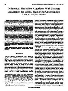
use the fitness value of best known solutions ( f (x* ) ) newly updated in [2]. The error values achieved when FES=5e+3, FES=5e+4, FES=5e+5 for the 24 test functions are listed in Tables I-IV. We record the FES needed in each run for finding a solution satisfying the successful condition [2] in Table V. The success rate, feasible rate, and success performance are also listed. The convergence maps of SaDE on functions 1-6, functions 7-12, functions 13-18, and functions 19-24 are plotted in Figures 1-4 respectively.
i = 1,…q max{gi ( x),0} i = q + 1,…, m hi (x)
Gi ( x) =
Therefore, the objective of our algorithm is to minimize the fitness function f (x) , at the same time the optimum solutions obtained must satisfy all the constraints Gi ( x) .
15
Among various constraints handling methods mentioned in the introduction, some methods based on superiority of feasible solutions, such as the approach proposed by Deb [5], has demonstrated promising performance, as indicated in [6][7] which deal with constraints using DE. Besides this, Deb’s selection criterion [5] has no parameter to fine-tune, which is also the motivation of our SaDE too - no fine-tuning of parameters as much possible. Hence, we incorporate this constraints handling technique as follows: During the selection procedure, the trial vector is compared to that of its corresponding target vector in the current population considering both the fitness value and constraints. The trial vector will replace the target vector and enter the population of the next generation if any of the following conditions is true. 1) The trial vector is feasible and the target vector is not. 2) The trial vector and target vector are both feasible and trial vector has smaller or equal fitness value (for minimization problem) than the corresponding target vector. 3) The trial vector and target vector are both infeasible, but trial vector has a smaller overall constrain violation. The overall constrain violation is a weighted mean value of all the constraints, which is expressed as following,
v( x) = where wi =
∑
m i =1
5
log(f(x)-f(x*))
0 -5 -10 -15 -20 -25 -30 -35
0
0.5
1
1.5
2
2.5 FES
3
3.5
4
4.5
8 g01 g02 g03 g04 g05 g06
6 4 2
log(v)
0 -2 -4 -6 -8
∑ i=1 wi m
-10
G max i is the
-12
0
0.5
1
1.5 FES
2
2.5
(1-b) log(v) vs FES Figure 1: Convergence Graph for Function 1-6
1 which varies during the G maxi
evolution in order to accurately normalize the constraints of the problem, thus the overall constrain violation can represent all constraints more equally. 20
5 5
x 10
(1-a) log(f(x)-f(x*)) vs FES
maximum violation of the constraints Gi (x) obtained so far. Here, we set wi as
g01 g02 g03 g04 g05 g06
10
wi (Gi ( x))
1 is a weighted parameter, G maxi
EXPERIMENTAL RESULTS
3 4
x 10
20
6 g07 g08 g09 g10 g11 g12
10
2 0
0
-2 log(v)
log(f(x)-f(x*))
g13 g14 g15 g16 g17 g18
4
-10
-4 -6
-20
-8 -10
-30
-12 -40
0
0.5
1
1.5
2
2.5 FES
3
3.5
4
4.5
-14
5
0
0.5
1
1.5 FES
5
x 10
2
2.5
3 4
x 10
(3-b) log(v) vs FES
(2-a) log(f(x)-f(x*)) vs FES
Figure 3 Convergence Graph for Function 13-18 15 g07 g08 g09 g10 g11 g12
10
10 g19 g20 g21 g22 g23 g24
5 0
log(f(x)-f(x*))
log(v)
5
0
-5 -10 -15
-5 -20
-10
-25
0
1000
2000
3000 FES
4000
5000
6000 -30
(2-b) log(v) vs FES
0
0.5
1
1.5
2
2.5 FES
3
3.5
4
4.5
5 x 10
5
(4-a) log(f(x)-f(x*)) vs FES
Figure 2 Convergence Graph for Function 7-12 25
g19 g20 g21 g22 g23 g24
20
10 g13 g14 g15 g16 g17 g18
log(f(x)-f(x*))
0
15 10
log(v)
5
-5
5 0
-10
-5
-15
-10 -15
-20
-25
0
0.5
1
1.5
2
2.5 FES
3
3.5
4
4.5
0
0.5
1
1.5
2
2.5 FES
3
3.5
4
4.5
5 5
x 10
(4-b) log(v) vs FES Figure 4 Convergence Graph for Function 19-24
5 5
x 10
(3-a) log(f(x)-f(x*)) vs FES
From the results, we could observe that, for all problems, the SaDE algorithm could reach the newly updated best known solutions except problems 20 and 22. As shown in Table V, the feasible rates of all problems are 21
100%, except problem 20 and 22. Problem 20 is highly constrained and no algorithm in the literature found feasible solutions. The successful rates are very encouraging, as most problems have 100%. Problems 2, 3, 10, 14, 18, 21 and 23 have 84%, 96%, 80%, 92%, 60% and 88% respectively. Problem 17 has 4%, with successfully finding better solution only once. Although the successful rate of problem 22 is 0, the result we obtained indeed is much better than previous best known solutions, and approximates the newly updated best known solutions. We set MAX_FES as 5e+5, however from the experiment results we could find that SaDE actually achieved the best known solutions within 5e+4 for many problems. We calculate the algorithm complexity according to [2] show in Table VI. We use Matlab 6.5 to implement the algorithm and the system configurations are:
[7]
Intel Pentium® 4 CPU 3.00 GHZ 2 GB of memory Windows XP Professional Version 2002 TABLE VI: COMPUTATIONAL COMPLEXITY
T1 4.9182
T2 8.3405
(T2-T1)/T1 0.6958
VI. CONCLUSION In this paper, we generalized the Self-adaptive Differential Evolution algorithm for handling optimization problem with multiple constraints, without introducing any additional parameters. The performance of our approach was evaluated on the testbed for CEC2006 special session on constrained real parameter optimization. The SaDE algorithm demonstrated effectiveness and robustness. REFERENCES [1]
[2]
[3] [4] [5] [6]
A. K. Qin and P. N. Suganthan, “Self-adaptive Differential Evolution Algorithm for Numerical Optimization” In: IEEE Congress on Evolutionary Computation (CEC 2005) Edinburgh, Scotland, Sep 02-05, 2005. J. J. Liang, T. P. Runarsson, E. Mezura-montes, M. Clerc, P.N.Suganthan, C. A. C. Coello, and K.Deb, “Problem Definitions and Evaluation Criteria for the CEC 2006 Special Session on Constrained Real-Paremeter Optimization,” Technical Report, 2005. http://www.ntu.edu.sg/home/EPNSugan Z. Michalewicz and M. Schoenauer, “Evolutionary Algorithms for Constrained Parameter Optimization Problems,” Evolutionary Computation, 4(1):1–32, 1996. R. Storn and K. V. Price, “Differential evolution-A simple and Efficient Heuristic for Global Optimization over Continuous Spaces,” Journal of Global Optimization 11:341-359. 1997. K. Deb. “An Efficient Constraint Handling Method for Genetic Algorithms”, Computer Methods in Applied Mechanics and Engineering, 186(2/4):311–338, 2000. J. Lampinen. “A Constraint Handling Approach for the Differential Evolution Algorithm.” In Proceedings of the Congress on Evolutionary Computation 2002 (CEC’2002), volume 2, pages 1468–1473, Piscataway, New Jersey, May 2002.
22
R. Landa-Becerra and C. A. C. Coello. “Optimization with Constraints using a Cultured Differential Evolution Approach.” In Proceedings of the Genetic and Evolutionary ComputationConference (GECCO'2005), volume 1, pages 27-34, New York, June 2005. Washington DC, USA, ACM Press.
TABLE I ERROR VALUES ACHIEVED WHEN FES= 5×10³ , FES= 5×10⁴, FES= 5×10⁵ FOR PROBLEMS 1-6 Prob. FES
5×10³
Best Median Worst c
5×10⁴
Mean Std Best Median Worst c
5×10⁵
Mean Std Best Median Worst c
v
v
v
Mean Std
g01
g02
g03
g04
g05
g06
2.9525e+000(0) 4.2828e+000(0) 5.2143e+000(0) 0, 0, 0 0 4.1779e+000 5.2257e-001 2.8414e-010(0) 2.9675e-010(0) 3.0000e-010(0) 0, 0, 0 0 2.9488e-010 4.9526e-012 0(0) 0(0) 0(0) 0, 0, 0 0 0 0
3.2958e-001(0) 3.7275e-001(0) 4.3843e-001(0) 0, 0, 0 0 3.7920e-001 2.9111e-002 4.2504e-003(0) 2.2353e-002(0) 3.8493e-002(0) 0, 0, 0 0 2.1825e-002 8.2730e-003 8.0719e-010(0) 3.0800e-009(0) 1.8353e-002(0) 0, 0, 0 0 2.0560e-003 4.9786e-003
3.3141e-001(0) 8.4884e-001(0) 8.8551e-001(1) 0, 0, 0 0 7.8931e-001 1.5394e-001 5.9753e-005(0) 9.9222e-004(0) 7.1664e-001(0) 0, 0, 0 0 6.2425e-002 1.5421e-001 1.3749e-010(0) 1.7770e-008(0) 1.3389e-004(0) 0, 0, 0 0 1.3532e-005 3.4743e-005
3.5714e+001(0) 7.5864e+001(0) 1.1877e+002(0) 0, 0, 0 0 7.7970e+001 2.1465e+001 2.5043e-007(0) 2.9835e-007(0) 3.3795e-007(0) 0, 0, 0 0 2.9795e-007 2.5148e-008 2.1667e-007(0) 2.1667e-007(0) 2.1667e-007(0) 0, 0, 0 0 2.1667e-007 1.8550e-012
2.2578e+001(3) 2.7489e+002(3) 1.0948e+002(3) 0, 1, 3 4.7389e-003 1.5908e+002 1.1344e+002 1.0004e-011(0) 5.2481e-004(0) 1.3955e-003(0) 0, 0, 0 0 6.3977e-004 5.4286e-004 0(0) 0(0) 0(0) 0, 0, 0 0 0 1.8190e-013
6.4548e+001(0) 3.4622e+002(0) 1.7502e+003(0) 0, 0, 0 0 4.3473e+002 3.6649e+002 4.5475e-011(0) 4.5475e-011(0) 4.5475e-011(0) 0, 0, 0 0 4.5475e-011 0 4.5475e-011(0) 4.5475e-011(0) 4.5475e-011(0) 0, 0, 0 0 4.5475e-011 0
TABLE II ERROR VALUES ACHIEVED WHEN FES= 5×10³ , FES= 5×10⁴, FES= 5×10⁵ FOR PROBLEMS 7-12 Prob.
g07
g08
g09
g10
g11
g12
5×10³
Best Median Worst c
5×10⁴
Mean Std Best Median Worst c
5×10⁵
Mean Std Best Median Worst c
3.8845e+000(0) 6.7238e+000(0) 1.2048e+001(0) 0, 0, 0 0 7.1258e+000 2.6450e+000 6.8221e-008(0) 2.7655e-003(0) 2.0290e-002(0) 0, 0, 0 0 4.9297e-003 5.9290e-003 6.8180e-008(0) 1.4608e-007(0) 6.3431e-005(0) 0, 0, 0 0 4.7432e-006 1.4993e-005
8.1964e-011(0) 8.1964e-011(0) 8.1964e-011(0) 0, 0, 0 0 8.1964e-011 1.0599e-017 8.1964e-011(0) 8.1964e-011(0) 8.1964e-011(0) 0, 0, 0 0 8.1964e-011 6.0492e-018 8.1964e-011(0) 8.1964e-011(0) 8.1964e-011(0) 0, 0, 0 0 8.1964e-011 3.8426e-018
4.1400e-001(0) 7.0402e-001(0) 1.8411e+000(0) 0, 0, 0 0 8.1345e-001 3.5365e-001 3.7440e-007(0) 7.1033e-007(0) 3.8943e-005(0) 0, 0, 0 0 4.4545e-006 8.7853e-006 3.7440e-007(0) 3.7440e-007(0) 3.7440e-007(0) 0, 0, 0 0 3.7440e-007 7.9851e-014
9.2363e+002(0) 1.4735e+003(0) 2.0997e+003(0) 0, 0, 0 0 1.4603e+003 2.7973e+002 1.9910e-006(0) 1.3888e-001(0) 3.4904e+000(0) 0, 0, 0 0 3.9758e-001 7.4290e-001 6.6393e-011(0) 1.8120e-006(0) 7.8300e-006(0) 0, 0, 0 0 1.6907e-006 1.5244e-006
3.3473e-004(0) 9.6840e-002(0) 2.1645e-001(0) 0, 0, 0 0 1.0756e-001 6.8547e-002 0(0) 0(0) 9.9985e-005(0) 0, 0, 0 0 9.3997e-006 2.7549e-005 0(0) 0(0) 0(0) 0, 0, 0 0 0 0
1.9651e-014(0) 1.2552e-012(0) 1.2816e-010(0) 0, 0, 0 0 1.0822e-011 2.6763e-011 0(0) 0(0) 0(0) 0, 0, 0 0 0 0 0(0) 0(0) 0(0) 0, 0, 0 0 0 0
FES
v
v
v
Mean Std
TABLE III ERROR VALUES ACHIEVED WHEN FES= 5×10³ , FES= 5×10⁴, FES= 5×10⁵ FOR PROBLEMS 13-18 Prob.
g13
g14
g15
g16
g17
g18
5×10³
Best Median Worst c
5×10⁴
Mean Std Best Median Worst c
9.4326e-001(3) 8.3030e-001(3) 5.2140e-001(3) 0, 2, 3 5.6738e-002 1.1713e+000 1.2511e+000 5.3102e-006(0) 8.3300e-006(0) 3.8491e-001(0) 0, 0, 0 0 1.0778e-001 1.7638e-001
4.3915e+000(3) 5.4314e+000(3) 2.4726e+000(3) 0, 3, 3 3.7325e-002 4.9550e+000 1.7242e+000 1.5331e-005(0) 1.4460e-004(0) 4.4106e-004(0) 0, 0, 0 0 1.6058e-004 1.0951e-004
6.6347e-002(2) 9.4042e-001(2) 1.6126e+000(2) 0, 1, 2 1.3524e-002 1.4324e+000 1.5740e+000 6.0822e-011(0) 6.8150e-005(0) 1.4563e-004(0) 0, 0, 0 0 6.3430e-005 6.0058e-005
2.8438e-002(0) 5.7669e-002(0) 1.1087e-001(0) 0, 0, 0 0 5.9573e-002 1.9716e-002 6.5214e-011(0) 6.5251e-011(0) 6.5455e-011(0) 0, 0, 0 0 6.5277e-011 6.7594e-014
9.1761e+001(4) 9.3311e+001(4) 9.5509e+001(4) 0, 3, 4 5.5918e-002 1.0664e+002 6.1893e+001 3.9816e+001(0) 7.4058e+001(0) 7.4058e+001(0) 0, 0, 0 0 7.2688e+001 6.8484e+000
1.2814e-001(0) 2.6913e-001(0) 4.1448e-001(0) 0, 0, 0 0 2.7886e-001 7.7546e-002 2.7581e-011(0) 1.0178e-010(0) 1.9163e-001(0) 0, 0, 0 0 1.5312e-002 5.2992e-002
FES
v
v
Mean Std
23
5×10⁵
Best Median Worst c
v
Mean Std
4.1898e-011(0) 4.1898e-011(0) 1.0696e-006(0) 0, 0, 0 0 8.0263e-008 2.7832e-007
TABLE IV
2.9050e-006(0) 1.4793e-005(0) 2.5233e-004(0) 0, 0, 0 0 4.6979e-005 6.4986e-005
6.0822e-011(0) 6.0822e-011(0) 6.0822e-011(0) 0, 0, 0 0 6.0822e-011 0
6.5214e-011(0) 6.5214e-011(0) 6.5214e-011(0) 0, 0, 0 0 6.5214e-011 0
8.1858e-011(0) 7.4058e+001(0) 7.4058e+001(0) 0, 0, 0 0 6.9670e+001 1.6168e+001
1.5561e-011(0) 1.5561e-011(0) 1.9104e-001(0) 0, 0, 0 0 1.5284e-002 5.2898e-002
ERROR VALUES ACHIEVED WHEN FES= 5×10³ , FES= 5×10⁴, FES= 5×10⁵ FOR PROBLEMS 19-24
Prob.
g19
g20
g21
g22
g23
g24
5×10³
Best Median Worst c
5×10⁴
Mean Std Best Median Worst c
5×10⁵
Mean Std Best Median Worst c
9.9842e+001(0) 1.5038e+002(0) 1.9265e+002(0) 0, 0, 0 0 1.4462e+002 2.2065e+001 5.8659e-007(0) 8.5695e-004(0) 1.1303e-001(0) 0, 0, 0 0 6.0660e-003 2.2429e-002 5.4456e-011(0) 1.3868e-010(0) 3.1141e-009(0) 0 0 4.2052e-010 7.2976e-010
1.2960e+001(20) 1.5603e+001(20) 1.3569e+001(20) 2, 18, 20 5.6112e+000 1.4265e+001 1.7690e+000 1.8020e-002(6) 5.1702e-001(19) 4.5755e+000(19) 1, 15, 19 1.5836e-001 2.1193e+000 2.4755e+000 1.8020e-002(6) 2.3757e-001(20) 5.3597e-001(20) 0, 16, 20 8.8255e-002 2.5564e-001 1.0638e-001
4.6515e+002(5) 3.9781e+002(5) 4.0739e+002(5) 0, 3, 5 6.3055e-002 4.1002e+002 1.2050e+002 4.6858e-002(0) 6.1550e-002(0) 6.2397e-002(0) 0, 0, 0 0 6.0340e-002 3.8090e-003 0(0) 2.5785e-008(0) 6.0712e-003(0) 0, 0, 0 0 7.6753e-004 1.5058e-003
1.6363e+004(19) 7.8714e+003(19) 1.3480e+004(19) 14, 19, 19 1.7472e+007 1.2034e+004 2.9316e+003 3.0199e+001(0) 1.0372e+002(0) 1.1282e+004(16) 0, 0, 0 0 5.3477e+003 6.2993e+003 1.9483e+000(0) 4.6907e+001(0) 1.2204e+002(0) 0, 0, 0 0 5.0203e+001 3.0415e+001
6.1159e+002(4) 2.8993e+002(4) 4.4529e+002(5) 0, 2, 4 6.0069e-003 4.0600e+002 8.0627e+001 7.6219e-003(0) 5.5090e-002(0) 5.5144e-002(0) 0, 0, 0 0 5.0237e-002 1.3633e-002 0(0) 3.9790e-013(0) 1.3788e-003(0) 0, 0, 0 0 1.2061e-004 3.4116e-004
1.7199e-005(0) 9.3936e-005(0) 1.7135e-004(0) 0, 0, 0 0 8.4004e-005 4.5396e-005 4.6372e-012(0) 4.6372e-012(0) 4.6372e-012(0) 0, 0, 0 0 4.6372e-012 0 4.6372e-012(0) 4.6372e-012(0) 4.6372e-012(0) 0, 0, 0 0 4.6372e-012 0
FES
v
v
v
Mean Std
Prob. g01 g02 g03 g04 g05 g06 g07 g08 g09 g10 g11 g12 g13 g14 g15 g16 g17 g18 g19 g20 g21 g22 g23 g24
TABLE VI NUMBER OF FES TO ACHIEVE THE FIXED ACCURACY LEVEL ( ( f(x) - f(x*)) ≤ 0.0001), SUCCESS RATE, FEASIBLE RATE AND SUCCESS PERFORMANCE Feasible Success Best Median Worst Mean Std Rate Rate 25115 25115 25115 25115 0 100% 100% 76915 128970 188990 142570 100% 84% 30000 261000 243520 135990 100% 96% 25107 25107 25113 25107 2 100% 100% 35500 65000 152000 74340 30484 100% 100% 12546 14404 18347 14394 1242 100% 100% 25195 101240 422860 143090 124800 100% 100% 782 1272 1775 1268 242 100% 100% 12960 16787 33166 18560 5170 100% 100% 26000 52000 153000 58760 33968 100% 100% 12643 25111 25120 23353 3482 100% 100% 463 1717 2576 1611 582 100% 100% 25161 25219 126080 42372 29775 100% 100% 32000 77000 154320 179040 100% 80% 25500 41500 97000 45240 18928 100% 100% 13144 14433 15797 14545 748 100% 100% 443000 497720 11400 100% 4% 26000 26000 65400 130870 100% 92% 25531 51588 78048 48733 13552 100% 100% 0% 0% 98500 320000 327660 166180 100% 60% 100% 0% 82500 298500 294540 137090 100% 88% 4280 4843 5657 4847 360 100% 100%
24
Success Performance 25115 183850 298960 25107 73000 12546 27637 1323 21446 44167 25111 2576 25168 45000 27000 14948 12500000 28261 52165 164170 129550 4624