Self-adaptive Integer and Decimal Mutation Operators for Genetic Algorithms Ghodrat Moghadampour, PhD Vaasa University of Applied Sciences Wolffintie 30 65200, Vaasa, Finland
[email protected]
1. INTRODUCTION ABSTRACT Evolutionary algorithms are affected by more parameters than optimization methods typically. This is at the same time a source of their robustness as well as a source of frustration in designing them. Adaptation can be used not only for finding solutions to a given problem, but also for tuning genetic algorithms to the particular problem. Adaptation can be applied to problems as well as to evolutionary processes. In the first case adaptation modifies some components of genetic algorithms to provide an appropriate form of the algorithm, which meets the nature of the given problem. These components could be any of representation, crossover, mutation and selection. In the second case, adaptation suggests a way to tune the parameters of the changing configuration of genetic algorithms while solving the problem. In this paper two new self-adaptive mutation operators; integer and decimal mutation are proposed for implementing efficient mutation in the evolutionary process of genetic algorithm for function optimization. Experimentation with 27 test cases and 1350 runs proved the efficiency of these operators in solving optimization problems.
Categories and Subject Descriptors I.2.2 [ArtiFicial Intelligence]: Automatic Programming| program synthesis, program modifcation
General Terms Algorithms, Theory, Design, Experimentation, Performance
Keywords Evolutionary algorithm, genetic algorithm, function optimization, mutation operator, self-adaptive mutation operators, integer mutation operator, decimal mutation operator, fitness evaluation and analysis
Evolutionary algorithms are heuristic algorithms, which imitate the natural evolutionary process and try to build better solutions by gradually improving present solution candidates. It is generally accepted that any evolutionary algorithm must have five basic components: 1) a genetic representation of a number of solutions to the problem, 2) a way to create an initial population of solutions, 3) an evaluation function for rating solutions in terms of their “fitness”, 4) “genetic” operators that alter the genetic composition of offspring during reproduction, 5) values for the parameters, e.g. population size, probabilities of applying genetic operators [9]. Genetic algorithm is an evolutionary algorithm, which starts the solution process by randomly generating the initial population and then refining the present solutions through natural like operators, like crossover and mutation. The behaviour of the genetic algorithm can be adjusted by parameters, like the size of the initial population, the number of times genetic operators are applied and how these genetic operators are implemented. Deciding on the best possible parameter values over the genetic run is a challenging task, which has made researchers busy with developing even better and efficient techniques than the existing ones.
2. GENETIC ALGORITHM Most often genetic algorithms (GAs) have at least the following elements in common: populations of chromosomes, selection according to fitness, crossover to produce new offspring, and random mutation of new offspring. A simple GA works as follows: 1) A population of l -bit strings (chromosomes) is randomly generated, 2) the fitness of each chromosome in the population is calculated, 3) chromosomes are selected to go through crossover and mutation operators with p c and p m probabilities respectively, 4) the old population is replace by the new one, 5) the process is continued until the termination conditions are met. However, more sophisticated genetic algorithms typically include other intelligent operators, which apply to the specific problem. In addition, the whole algorithm is normally implemented in a novel way with user-defined features while for instance measuring and controlling parameters, which affect the behaviour of the algorithm.
2.1 Genetic Operators For any evolutionary computation technique, the representation of an individual in the population and the set of operators used to alter its genetic code constitute probably the two most important components of the system. Therefore, an appropriate representation (encoding) of problem variables must be chosen along with the appropriate evolutionary computation operators. The reverse is also true; operators must match the representation. Data might be represented in different formats: binary strings, real-valued vectors, permutations, finite-state machines, parse trees and so on. Decision on what genetic operators to use greatly depends on the encoding strategy of the GA. For each representation, several operators might be employed [9]. The most commonly used genetic operators are crossover and mutation. These operators are implemented in different ways for binary and real-valued representations. In the following, these operators are described in more details.
2.1.1 Crossover Crossover is the main distinguishing feature of a GA. The simplest form of crossover is single-point: a single crossover position is chosen randomly and the parts of the two parents after the crossover position are exchanged to form two new individuals (offspring). The idea is to recombine building blocks (schemas) on different strings. However, single-point crossover has some shortcomings. For instance, segments exchanged in the singlepoint crossover always contain the endpoints of the strings; it treats endpoints preferentially, and cannot combine all possible schemas. For example, it cannot combine instances of 11*****1 and ****11** to form an instance of 11***11*[10]. Moreover, the single-point crossover suffers from “positional bias” [10]: the location of the bits in the chromosome determines the schemas that can be created or destroyed by crossover. Consequently, schemas with long defining lengths are likely to be destroyed under single-point crossover. The assumption in singlepoint crossover is that short, low-order schemas are the functional building blocks of strings, but the problem is that the optimal ordering of bits is not known in advance [10]. Moreover, there may not be any way to put all functionally related bits close together on a string, since some particular bits might be crucial in more than one schema. This might happen if for instance in one schema the bit value of a locus is 0 and in the other schema the bit value of the same locus is 1. Furthermore, the tendency of singlepoint crossover to keep short schemas intact can lead to the preservation of so-called hitchhiker bits. These are bits that are not part of a desired schema, but by being close on the string, hitchhike along with the reproduced beneficial schema [10]. In two-point crossover, two positions are chosen at random and the segments between them are exchanged. Two-point crossover reduces positional bias and endpoint effect, it is less likely to disrupt schemas with large defining lengths, and it can combine more schemas than single-point crossover [10]. Two-point crossover has also its own shortcomings; it cannot combine all schemas. Multipoint-crossover has also been implemented, e.g. in one method, the number of crossover points for each parent is chosen from a Poisson distribution whose mean is a function of the length of the chromosome. Another method of implementing multipointcrossover is the “parameterized uniform crossover” in which each bit is exchanged with probability p , typically 0.5 p 0.8
[10]. In parameterized uniform crossover, any schemas contained at different positions in the parents can potentially be recombined in the offspring; there is no positional bias. This implies that uniform crossover can be highly disruptive of any schema and may prevent coadapted alleles from ever forming in the population [10]. There has been some successful experimentation with a crossover method, which adapts the distribution of its crossover points by the same process of survival of the fittest and recombination [9]. This was done by inserting into the string representation special marks, which keep track of the sites in the string where crossover occurred. The hope was that if a particular site produces poor offspring, the site dies off and vice versa. The one-point and uniform crossover methods have been combined by some researchers through extending a chromosomal representation by additional bit. There has also been some experimentation with other crossovers: segmented crossover and shuffle crossover [4], [9]. Segmented crossover, a variant of the multipoint, allows the number of crossover points to vary. The fixed number of crossover points and segments (obtained after dividing a chromosome into pieces on crossover points) are replaced by a segment switch rate, which specifies the probability that a segment will end at any point in the string. The shuffle crossover is an auxiliary mechanism, which is independent of the number of the crossover points. It 1) randomly shuffles the bit positions of the two strings in tandem, 2) exchanges segments between crossover points, and 3) unshuffles the string [9]. In gene pool recombination, genes are randomly picked from the gene pool defined by the selected parents. There is no definite guidance on when to use which variant of crossover. The success or failure of a particular crossover operator depends on the particular fitness function, encoding, and other details of GA. Actually, it is a very important open problem to fully understand interactions between particular fitness function, encoding, crossover and other details of a GA. Commonly, either two-point crossover or parameterized uniform crossover has been used with the probability of occurrence p 0.7 0.8 [10]. Generally, it is assumed that crossover is able to recombine highly fit schemas. However, there is even some doubt on the usefulness of crossover, e.g. in schema analysis of GA, crossover might be considered as a “macro-mutation” operator that simply allows for large jumps in the search space [10].
2.1.2 Mutation The common mutation operator used in canonical genetic algorithms to manipulate binary strings a (a1 ,... a ) I {0,1} of fixed length was originally introduced by Holland [6]for general finite individual spaces I A1 ... A , where
Ai { i1 ,..., ik } . By this definition, the mutation operator l
proceeds by: i.
determining the position i1 ,..., ih (i j {1,..., l}) to undergo
mutation by a uniform random choice, where each position has the same small probability p m of undergoing mutation, independently of what happens at other position ii. forming the new vector
ai (a1 ,..., ai11 , ai , ai11 ,..., ai 1 , ai , ai 1 ,... a ) , 1 h h h
where
ai Ai is drawn uniformly at random from the set of
admissible values at position i . The original value a i at a position undergoing mutation is not excluded from the random choice of ai Ai . This implies that although the position is chosen for mutation, the corresponding value might not change at all [2]. Mutation rate is usually very small, like 0.001 [10]. A good starting point for the bit-flip mutation operation in binary encoding is Pm 1 L , where L is the length of the chromosome [12]. Since 1
corresponds to flipping one bit per genome on L average, it is used as a lower bound for mutation rate. A mutation rate of range Pm 0.005,0.01 is recommended for binary encoding [16]. For real-value encoding the mutation rate is usually Pm 0.6,0.9 and the crossover rate is Pm 0.7,1.0 [16]. Crossover is commonly viewed as the major instrument of variation and innovation in GAs, with mutation, playing a background role, insuring the population against permanent fixation at any particular locus [10], [2]. Mutation and crossover have the same ability for “disruption” of existing schemas, but crossover is a more robust constructor of new schemas [15], [10]. The power of mutation is claimed to be underestimated in traditional GA, since experimentation has shown that in many cases a hill-climbing strategy works better than a GA with crossover [12], [10]. While recombination involves more than one parent, mutation generally refers to the creation of a new solution form one and only one parent. Given a real-valued representation where each element in a population is an n -dimensional vector x n , there are many methods for creating new offspring using mutation. The general form of mutation can be written as: x m(x) ,
(1)
where x is the parent vector, m is the mutation function and x is the resulting offspring vector. The more common form of mutation generated offspring vector: x x M ,
(2)
where the mutation M is a random variable. M has often zero mean such that E( x) x .
(3)
the expected difference between the real values of a parent and its offspring is zero [2]. Some forms of evolutionary algorithms apply mutation operators to a population of strings without using recombination, while other algorithms may combine the use of mutation with recombination. Any form of mutation applied to a permutation must yield a string, which also presents a permutation. Most mutation operators for permutations are related to operators, which have also been used in neighbourhood local search strategies [17]. Some other variations of the mutation operator for more specific problems have been introduced in Chapter 32 in [2]. Some new methods and techniques for applying crossover and mutation operators have also been presented in [11].
It is not a choice between crossover and mutation but rather the balance among crossover, mutation, selection, details of fitness function and the encoding. Moreover, the relative usefulness of crossover and mutation change over the course of a run. However, all these remain to be elucidated precisely [10].
2.1.3 Other Operators and Mating Strategies In addition to common crossover and mutation there are some other operators used in GAs including inversion, gene doubling and several operators for preserving diversity in the population. For instance, a “crowding” operator has been used in [3], [10] to prevent too many similar individuals (“crowds”) from being in the population at the same time. This operator replaces an existing individual by a newly formed and most similar offspring. In [7] a probabilistic crowding niching algorithm in which subpopulations are maintained reliably, is presented. It is argued that like the closely related deterministic crowding approach, probabilistic crowding is fast, simple, and requires no parameters beyond those of classical genetic algorithms. The same result can be accomplished by using an explicit “fitness sharing” function [10], whose idea is to decrease each individual’s fitness by an explicit increasing function of the presence of other similar population members. In some cases, this operator induces appropriate “speciation”, allowing the population members to converge on several peaks in the fitness landscape [10]. However, the same effect could be obtained without the presence of an explicit sharing function [14], [10]. Diversity in the population can also be promoted by putting restrictions on mating. For instance, distinct “species” tend to be formed if only sufficiently similar individuals are allowed to mate [10]. Another attempt to keep the entire population as diverse as possible is disallowing mating between too similar individuals, “incest” [4], [10]. Another solution is to use a “sexual selection” procedure; allowing mating only between individuals having the same “mating tags” (parts of the chromosome that identify prospective mates to one another). These tags, in principle, would also evolve to implement appropriate restrictions on new prospective mates [5]. Another solution is to restrict mating spatially. The population evolves on a spatial lattice, and individuals are likely to mate only with individuals in their spatial neighborhoods. Such a scheme would help preserve diversity by maintaining spatially isolated species, with innovations largely occurring at the boundaries between species [10]. The efficiency of genetic algorithms has also been tried by imposing adaptively, where the algorithm operators are controlled dynamically during runtime [5]. These methods cn be categorized as deterministic, adaptive, and self-adaptive methods [1], [5]. Adaptive methods adjust the parameters’ values during runtime based on feedbacks from the algorithm [5], which are mostly based on the quality of the solutions or speed of the algorithm [13].
2.1.4 Other Operators and Mating Strategies In addition to common crossover and mutation there are some other operators used in GAs including inversion, gene doubling and several operators for preserving diversity in the population. For instance, a “crowding” operator has been used in [3], [10] to prevent too many similar individuals (“crowds”) from being in the population at the same time. This operator replaces an existing individual by a newly formed and most similar offspring. In [7] a
probabilistic crowding niching algorithm in which subpopulations are maintained reliably, is presented. It is argued that like the closely related deterministic crowding approach, probabilistic crowding is fast, simple, and requires no parameters beyond those of classical genetic algorithms. The same result can be accomplished by using an explicit “fitness sharing” function [10], whose idea is to decrease each individual’s fitness by an explicit increasing function of the presence of other similar population members. In some cases, this operator induces appropriate “speciation”, allowing the population members to converge on several peaks in the fitness landscape [10]. However, the same effect could be obtained without the presence of an explicit sharing function [14], [10].
Apparently, changes of different magnitudes are required at different stages of the evolutionary process. Thus, two types of decimal mutation operators have been implemented: 1.
For modifying variables with integer values. The bounds for the absolute values of such changes are at least 1 and at most the integer part of the real value representation of the variable. This means that the upper bound of the range may vary even for each variable of the same individual. The randomly selected mutation value may be either positive or negative. Thus, if the integer part of the variable is int(variable) , the integer mutation range is 1, int(variable) .
Diversity in the population can also be promoted by putting restrictions on mating. For instance, distinct “species” tend to be formed if only sufficiently similar individuals are allowed to mate [10]. Another attempt to keep the entire population as diverse as possible is disallowing mating between too similar individuals, “incest” [4], [10]. Another solution is to use a “sexual selection” procedure; allowing mating only between individuals having the same “mating tags” (parts of the chromosome that identify prospective mates to one another). These tags, in principle, would also evolve to implement appropriate restrictions on new prospective mates [5]. Another solution is to restrict mating spatially. The population evolves on a spatial lattice, and individuals are likely to mate only with individuals in their spatial neighborhoods. Such a scheme would help preserve diversity by maintaining spatially isolated species, with innovations largely occurring at the boundaries between species [10]. The efficiency of genetic algorithms has also been tried by imposing adaptively, where the algorithm operators are controlled dynamically during runtime [5]. These methods cn be categorized as deterministic, adaptive, and self-adaptive methods [1], [5]. Adaptive methods adjust the parameters’ values during runtime based on feedbacks from the algorithm [5], which are mostly based on the quality of the solutions or speed of the algorithm [13].
3. Self-adaptive Mutation Operators One major problem with the classical implementation of binary mutation, the multipoint mutation or the crossover operator is that it is difficult to control their effect or to restrict changes caused by them within certain values. Therefore, several techniques are developed here to implement the genetic operators intelligently so that the resulting modifications on the binary string will cause changes in the real values within the desired limits. This idea is implemented so that the real value of the variable is randomly changed within the desired limits and the modified value then is converted to the binary representation and stored as the value of the variable. In this way we can cause more precise mutations in the bit strings and make sure that changes in real values are within the desired bounds.
2.
For modifying variables with values from the range 0,1 . The lower bound for the absolute value of such changes is determined by the required precision of the real value presentation of the variable, like 106 . The upper bound for the absolute value of such changes is determined by decimal part of the variable. Here also the mutation value can be either positive or negative. Thus, if the number of digits after the decimal point for a variable is precision(variable ) , and the decimal part of the variable is decimal(var iable) , the range for the real mutation values is precision( var iable ) 10 , decimal(var iable) .
3.1 The Integer Mutation Operator The integer mutation (IM) operator mutates the individuals of the population in relatively great magnitudes. This operator is naturally applied only to individuals with integer part equal or greater or than 1. During this operation an integer mutation value is selected randomly from the following range:
1, i nt(variable)
(4)
and added to the variable under mutation. Here, i nt(variable) stands for the absolute value of the integer part of the variable. Clearly, this integer part does not necessarily cover the whole range of the variable. To avoid wasting resources special care is taken to make sure that the generated random number is not 0. Thus, the upper bound for the integer mutation value is different for each variable and is defined by the absolute value of the integer part of the variable. This will make the process more flexible and smart. If the resulting value of the variable is outside of its pre-defined variable range, the change will be rejected. If the upper bound of the mutation value is set to a fixed value, the operator becomes inefficient or the probability for its failure will rise. For instance, if the optimal value of a variable is 0.05 and its present value 80.64, we will need 80 successful integer mutations of magnitude 1 in order to get close to the optimal value of the variable. However, if the magnitude of the integer mutation value can be dynamically determined by the magnitude of the variable, the operator will have a much greater chance to improve the value of the variable dramatically in a short time. During this operation a randomly generated integer number within the specified bounds is added to the value of the variable and the binary representation of the resulting offspring is updated. The
offspring is then evaluated and put through the survivor selection procedure. There is no fixed rate for this operator. All population members go through this operator at least once.
3.2 The Decimal Mutation Operator The decimal mutation (DM) operator is used in order to implement changes of smaller magnitudes on individuals. This operator is naturally applied only to variables with decimal part greater than 0. During this operation non-zero decimal numbers in the specific range are randomly generated and added to the randomly selected variables in the individual. The upper bound for the decimal mutation values is determined by the absolute value of the decimal part of variables. If the decimal part of a variable is denoted by decimal(variable) , the maximum distance of the mutation values from 0 is decimal(variable) . The lower bound of the mutation range is determined by the number of digits after the decimal point. Thus, if precision(variable) shows the number of required decimal places of a variable, the decimal mutation value is determined in the following way:
10 precision(variable ) , decimal(var iable)
(5)
Table 1. Summary of test runs with three different operator sets: CoMu (crossover & mutation), CoMuImDm (crossover, mutation, integer mutation & decimal mutation) and ImDm (integer mutation & decimal mutation) to solve Ackely’s functions (A1-A50), Colville’s function (C4), Grienwank’s functions (G1-G50), Rastrigin’s function (Ra1-Ra50), Rosenbrock’s function (Ro1-Ro50), Schaffer’s F6 (S62) and F7 (S72) functions. Fn. stands for function, F. for fitness and FE. for function evaluation. Fn.
Operator Set CoMu
If the resulting value of the variable is outside of the pre-defined range of the variable, the change will be rejected. The difference between this operator and the integer mutation operator is the way the mutation value is determined. Otherwise, these operators are similar. After each operator application, new offspring are evaluated and compared to the population individuals. Newly generated offspring will replace the worst individual in the population if they are better than the worst individual. Therefore, the algorithm is a steady state genetic algorithm.
4. EXPERIMENTATION The self-adaptive integer and decimal mutation operators were applied as part of a genetic algorithm to solve the following minimization problems: Ackley’s function, Colville’s function, Griewank’s function F1, Rastrigin’s function, Rosenbrock’s function and Schaffer’s F6 and F7 functions. For multidimensional problems with optional number of dimensions ( n ), the algorithm was tested for n 1, 2, 3, 5, 10, 50 . The population size was set to 9. The efficiency of the proposed operators was compared against classical crossover (with 55%- 88% crossover rate) and mutation operator (with 1% mutation rate). Experimentations were carried out with three different configurations. In the first configuration only classical mutation and crossover operators were used to solve the problems. In the second configuration classical mutation and crossover and proposed self-adaptive integer and decimal mutation operators were used to solve the problems. Finally, in the third configuration only proposed self-adaptive integer and decimal mutation operators were used to solve the problems. For each configuration the worst individual in the population was replaced by a better offspring produced as a result of applying an operator. Each algorithm was run 50 times for each problem. The following table summarises the results of applying three different sets of operators to solve functions mentioned earlier. Functions and different variations of their variables make 27 different test cases.
F.
CoMuIm_Dm
ImDm
FE.
F.
FE.
F.
FE.
A1
1.12E-06
5804
8.00E-08
3276
4.00E-06
10005
A2
2.98E-01
10017
1.76E-06
8174
4.00E-06
10005
A3
1.440
10009
8.30E-01
9844
8.02E-01
10006
A5
4.390
10015
0.278
10010
1.89
10006
A10
9.495
10009
1.188
10011
3.86
10006
A50
18.754
10019
8.925
10013
10.17
10005
C4
5.486
10012
0.564
5380
1.57
6688
G1
1.10E-03
5960
0.000
1740
7.89E-04
2723
G2
0.022
9998
0.017
9391
0.036
9644
G3
0.147
10017
0.110
10012
0.633
10005
G5
0.911
10007
0.531
10008
1.273
10004
G10
5.412
10006
2.860
10014
5.248
10006
G50
349.603
10018
56.67
10005
88.485
10006
Ra1
0.000
2650
0.000
494
0.00E+00
177
Ra2
0.073
9772
0.000
1111
0.00E+00
695
Ra3
0.593
10020
0.000
1867
0.239
4268
Ra5
2.951
10014
0.388
6300
2.688
9617
Ra10
19.720
10020
3.987
9417
9.830
10006
Ra50
149.98
10154
119.41
10076
114.50
10008
Ro1
0.000
18
6.46E-06
9832
5.56E-05
10008
Ro2
11.61
10013
5.32E-04
8259
3.56E-05
8474
Ro3
39.21
10010
0.111
10008
1.48
10008
Ro5
1.96E+04
10006
55.95
10012
116.87
10008
Ro10
3.29E+04
10011
1576
10026
9651
10008
Ro50
8.55E+07
10112
3.87E+05
10144
4.58E+07
10006
S62
1.07E-02
8746
5.05E-03
6822
3.69E-03
4807
S72
5.28E-02
7976
0.00E+00
780
0.00E+00
388
Studying results in Table 1 reveals that the integer and decimal mutation operators have successfully managed to improve the efficiency of the algorithm either by decreasing the required
number of function evaluations or improving the quality of the solutions or by resulting in both improvements simultaneously. Using the integer and decimal mutation operators in conjunction with classical crossover and mutation operators resulted in better fitness values in 93% of test cases and in less required function evaluations in 74% of test case. Furthermore, using integer and decimal mutation operators in combination with the crossover and mutation operator improved the quality of the solution by at least 90% in 44% of test cases. The integer and decimal mutation operators proved to outperform the classical crossover and mutation operators in 78% of test cases in terms of the quality of the solution and in 85% of test cases in terms of required function evaluations. In 56% of test cases the integer and decimal mutation operators resulted in at least 50% of improvement in the quality of solutions than the classical crossover and mutation operators.
5. CONCLUSIONS Two new genetic operators namely integer and decimal mutation operators were proposed in this paper. The operators were described and tested for solving some classical minimization problems. Furthermore, the efficiency of the proposed operators against the classical crossover and mutation operators was tested. Experimentation proved that the proposed operators are efficient and can lead into better results in solving optimization problems.
6. REFERENCES [1]
A. Eiben and J. Smith 2007. Introduction to Evolutionary Computing. Natural Computing Series. Springer, 2nd edition.
[2]
Bäck, Thomas, David B. Fogel, Darrell Whitely & Peter J. Angeline 2000. Mutation operators. In: Evolutionary Computation 1, Basic Algorithms and Operators. Eds T. Bäck, D.B. Fogel & Z. Michalewicz. United Kingdom: Institute of Physics Publishing Ltd, Bristol and Philadelphia. ISBN 0750306645.
[3] De Jong, K. A. 1975. An Analysis of the Behavior of a Class of Genetic Adaptive Systems. Ph.D. thesis, University of Michigan. Michigan: Ann Arbor. [4] Eshelman, L. J. & J.D. Schaffer 1991. Preventing premature convergence in genetic algorithms by preventing incest. In Proceedings of the Fourth International Conference on Genetic Algorithms. Eds R. K. Belew & L. B. Booker. San Mateo, CA : Morgan Kaufmann Publishers. [5] G. Eiben and M. C. Schut 2008. New Ways To Calibrate Evolutionary Algorithms. In Advances in Metaheuristics for Hard Optimization, pages 153–177.
[6] Holland, J. H. 1975. Adaptation in Natural and Artificial Systems. Ann Arbor: MI: University of Michigan Press. [7] Mengshoel, Ole J. & Goldberg, David E. 2008. The crowding approach to niching in genetic algorithms. Evolutionary Computation, Volume 16 , Issue 3 (Fall 2008). ISSN:1063-6560. [8] Michalewicz, Zbigniew 1996. Genetic Algorithms + Data Structures = Evolution Programs. Third, Revised and Extended Edition. USA: Springer. ISBN 3-540-60676-9. [9] Michalewicz, Zbigniew 2000. Introduction to search operators. In Evolutionary Computation 1, Basic Algorithms and Operators. Eds T. Bäck, D.B. Fogel & Z. Michalewicz. United Kingdom: Institute of Physics Publishing Ltd, Bristol and Philadelphia. ISBN 0750306645. [10] Mitchell, Melanie 1998. An Introducton to Genetic Algorithms. United States of America: A Bradford Book. First MIT Press Paperback Edition. [11] Moghadampour, Ghodrat 2006. Genetic Algorithms, Parameter Control and Function Optimization: A New Approach. PhD dissertation. ACTA WASAENSIA 160, Vaasa, Finland. ISBN 952-476-140-8. [12] Mühlenbein, H. 1992. How genetic algorithms really work: 1. mutation and hill-climbing. In: Parallel Problem Solving from Nature 2. Eds R. Männer & B. Manderick. NorthHolland. [13] S. K. Smit and A. E. Eiben 2009. Comparing Parameter Tuning Methods for Evolutionary Algorithms. In IEEE Congress on Evolutionary Computation (CEC), pages 399– 406, May 2009. [14] Smith, R. E., S. Forrest & A.S. Perelson 1993. Population diversity in an immune system model: implications for genetic search. In Foundations of Genetic Algorithms 2. Ed. L.D. Whitely. Morgan Kaufmann. [15] Spears, W. M. 1993. Crossover or mutation? In: Foundations of Genetic Algorithms 2. Ed. L. D. Whitely. Morgan Kaufmann. [16] [Ursem, Rasmus K. 2003. Models for Evolutionary Algorithms and Their Applications in System Identification and Control Optimization (PhD Dissertation). A Dissertation Presented to the Faculty of Science of the University of Aarhus in Partial Fulfillment of the Requirements for the PhD Degree. Department of Computer Science, University of Aarhus, Denmark. [17] Whitley, Darrell 2000. Permutations. In Evolutionary Computation 1, Basic Algorithms and Operators. Eds T. Bäck, D.B. Fogel & Z. Michalewicz. United Kingdom: Institute of Physics Publishing Ltd, Bristol and Philadelphia. ISBN 0750306645.