Self-Adaptive Revised Land Use Regression Models for ... - MDPI

sustainability Article

Self-Adaptive Revised Land Use Regression Models for Estimating PM2.5 Concentrations in Beijing, China Lujin Hu 1, *, Jiping Liu 1 and Zongyi He 2 1 2

*

Research Center of Government Geographic Information System, Chinese Academy of Surveying & Mapping, Beijing 100830, China; [email protected] School of Resource & Environmental Sciences, Wuhan University, Wuhan 430072, China; [email protected] Correspondence: [email protected]; Tel.: +86-10-6388-0566

Academic Editor: Daniel A. Vallero Received: 8 March 2016; Accepted: 4 August 2016; Published: 11 August 2016

Abstract: Heavy air pollution, especially fine particulate matter (PM2.5 ), poses serious challenges to environmental sustainability in Beijing. Epidemiological studies and the identification of measures for preventing serious air pollution both require accurate PM2.5 spatial distribution data. Land use regression (LUR) models are promising for estimating the spatial distribution of PM2.5 at a high spatial resolution. However, typical LUR models have a limited sampling point explanation rate (SPER, i.e., the rate of the sampling points with reasonable predicted concentrations to the total number of sampling points) and accuracy. Hence, self-adaptive revised LUR models are proposed in this paper for improving the SPER and accuracy of typical LUR models. The self-adaptive revised LUR model combines a typical LUR model with self-adaptive LUR model groups. The typical LUR model was used to estimate the PM2.5 concentrations, and the self-adaptive LUR model groups were constructed for all of the sampling points removed from the typical LUR model because they were beyond the prediction data range, which was from 60% of the minimum observation to 120% of the maximum observation. The final results were analyzed using three methods, including an accuracy analysis, and were compared with typical LUR model results and the spatial variations in Beijing. The accuracy satisfied the demands of the analysis, and the accuracies at the different monitoring sites indicated spatial variations in the accuracy of the self-adaptive revised LUR model. The accuracy was high in the central area and low in suburban areas. The comparison analysis showed that the self-adaptive LUR model increased the SPER from 75% to 90% and increased the accuracy (based on the root-mean-square error) from 20.643 µg/m3 to 17.443 µg/m3 for the PM2.5 concentrations during the winter of 2014 in Beijing. The spatial variation analysis for Beijing showed that the PM2.5 concentrations were low in the north, especially in the northwest region, and high in the southern and central portions of Beijing. This spatial variation was consistent with the fact that the northern region is mountainous and has fewer people and less traffic, which results in lower air pollution, than in the central region, which has a high population density and heavy traffic. Moreover, the southern region is adjacent to Hebei province, which contains many polluting enterprises; thus, this area exhibits higher air pollution levels than Beijing. Therefore, the self-adaptive revised LUR model is effective and reliable. Keywords: self-adaptive; land use regression; fine particulate matter; PM2.5 ; accuracy; spatial variation

1. Introduction Sustainability is important for human living environment, but the heavy air pollution in developed cities (e.g., Beijing in China), makes environmental sustainability more difficult to achieve. Thus, effective measures of preventing air pollution are indispensable to achieving sustainability. Accurate air pollution distribution is the analysis base for effective measures of preventing air Sustainability 2016, 8, 786; doi:10.3390/su8080786

www.mdpi.com/journal/sustainability

Sustainability 2016, 8, 786

2 of 23

pollution, especially PM2.5 pollution, which is the most serious air pollutant. Specifically, accurate PM2.5 pollution distribution can help us find the PM2.5 pollution level in different regions and hence make corresponding protection measures. In addition, the regions discovered to have heavy air pollution should strengthen air protection through policies and regulations, exploration of new green energy sources, and individual efforts. Fine particulate matter (PM2.5 ) consists of particles less than 2.5 µm that are suspended in the atmosphere in solid or liquid form [1]. Because of their irregular shape, small size, and strong enrichment effect, PM2.5 can easily enter the human body through respiratory bronchioles and alveoli and penetrate the blood, leading to respiration, circulation, immunity, endocrine, and central nervous systems problems and causing carcinogenic, teratogenic, mutagenic, and skin diseases. Currently, PM2.5 is the dominant form of air pollution and cause of adverse health effects [2–4]. According to epidemiological studies, the adverse health effects of long-term exposure to air pollution are associated with morbidity [5,6], mortality [7–12], low birth rate [13–16], short life expectancy [17,18], and population burden of disease [19,20]. In Beijing, which is the capital of China, PM2.5 pollution is two to three times higher than the World Health Organization (WHO) Level 1 Interim Target [21]. To persistently and effectively control environmental pollution, the Beijing Municipal Government has enacted vehicle use restrictions [22] and closed several polluting enterprises. In addition, the Beijing municipal environmental monitoring center has established air quality monitoring points in different regions of the city. However, only 35 monitoring points were established [23], and the established points are not evenly distributed throughout Beijing. Hence, it is difficult to determine the accurate distribution of urban PM2.5 , although epidemiological studies always require highly accurate information regarding the spatial variability of PM2.5 [24]. Therefore, we must use existing environmental monitoring data to estimate the environmental quality of unknown regions. Among the available estimation methods, land use regression (LUR) modeling is one of the best approaches [10]. Briggs [25] proposed applying the LUR model to environmental pollution mapping. Since then, the LUR model has been widely used to study the spatial distribution of environmental pollutants (such as fine particulate pollutants [24,26–29], black carbon [30,31], NO2 [12,32–34], NOx [12], and O3 [35]). The LUR model uses geographic information systems (i.e., spatial analysis, spatial overlay, and buffer analysis) to compute the quantitative values of several predictor variables (such as land use, road traffic, and terrain variables) for specific buffers. In this case, the predictor variable is considered as the independent variable and the air pollutant concentration is considered as the dependent variable to establish a regression model that is combined with a spatial interpolation method (such as Kriging and inverse distance weighing) to predict the air pollutant concentrations in regions without monitoring sites. Numerous studies have used LUR models to focus on the following aspects: model improvement, spatio-temporal analysis of PM2.5 distributions, and the links between PM2.5 pollution and public health. The studies for the model improvement have aimed to improve the accuracy of the typical LUR model. For example, a hybrid approach was proposed in which a typical LUR model and a machine learning method were selected and combined the Bayesian Maximum Entropy (BME) interpolation of the LUR space–time residuals [24]. A novel LUR model was proposed using data generated from a dispersion model instead of available monitoring data [36]. Moreover, LUR models and dispersion modeling methods were compared to determine the most appropriate approaches for specific areas and specific air pollutants [37]. Spatio-temporal analysis has also been the focus of many recent works because different time scales can be applied for spatio-temporal analysis when using LUR models. For example, yearly data were used to analyze the temporal variations in Taibei [38]. A two-stage spatio-temporal model was developed to predict daily fine particulate matter distributions [29]. Moreover, real-time hourly data were used to formulate separate morning and afternoon models [2]. Another focus of LUR model studies is the association between PM2.5 concentrations and public health. For example, the LUR was used to determine the association between natural mortality and mortality due to long-term exposure to the elemental components of particulate matter [11]. In addition, a national LUR model was generated to evaluate the associations between long-term


3 of 23

exposure to air pollution and non-accidental mortality and the mortality resulting from specific causes in the Netherlands [39]. All of these studies have resolved problems. However, some challenges remain for the LUR modeling community regarding the application of LUR models. One of the most important of these challenges is obtaining an accurate sampling point explanation rate (SPER, i.e., the rate of the sampling points with reasonable predicted concentrations to the total number of sampling points) for LUR models. However, the SPER is limiting for all the sampling locations when using LUR, especially for fine spatial scale analysis, e.g., the LUR models for interurban areas [40]. In addition, the SPER is low when estimating PM2.5 in Beijing and results in some negative concentration estimations, which is not consistent with the fact that the minimum PM2.5 concentration should be zero [41]. In some recent studies, attempts were made to improve the accuracy of PM2.5 estimates by using the following two approaches: (1) adding more predictor variables, e.g., on-road mobile emissions and stationary emissions data were added to LUR models in [27], satellite data were added in [33], and industry, commerce, and construction activities were added in [42]; and (2) combining LUR models with other models, e.g., a dispersion model in [36], and the Bayesian maximum entropy method in [38]. The first approach has more restrictions because the use of different regions in different countries results in different types of variables. Meanwhile, data regarding some air pollution predictors cannot be obtained because these data are not open-source. For the second approach, current studies have focused on combining LUR models with other estimation methods; however, this method requires more work than the first approach and only focuses on specific applications. Recognizing the above challenges, a self-adaptive revised LUR models were proposed herein to obtain higher SPERs for sampling locations in the target region to improve the accuracy of the LUR models. Specifically, we combined self-adaptive LUR groups for the removed sampling locations during the general LUR (typical LUR) model screening. For the typical LUR model, if the model accuracy was not sufficiently high for the predicted concentrations (e.g., the predicted results included multiple negative values estimated by LUR in [41]), the minimum predicted concentration should be zero and should be removed from the model. However, in this study, we constructed self-adaptive LUR models to address this issue based on exiting predictor variables and predicted concentrations. Self-adaptive means that a multivariable regression model is adapted to the independent variables at individual sampling locations; thus, a specific LUR model can be constructed for every sampling location. 2. Materials and Methods 2.1. Study Area Beijing is the capital of China and is located in the northern part of the North China Plain (39˝ 561 N and 116˝ 201 E). Beijing is surrounded by Tianjin Municipality to the east and Hebei Province to the north, west, and south and covers a total area of 16,410.54 square km with 16 districts and counties. By June 2015, the population in Beijing reached 21.689 million. Beijing is located in a warm temperate zone with a semi-humid climate and four distinctive seasons: spring, autumn, summer, and winter. Hot and wet conditions occur during the summer, and cold and dry conditions persist throughout the winter. Air pollution is more serious in Beijing during the winter because pollution is emitted from traffic, industries, coal combustion, and biomass combustion for cooking and winter heating [43]. In‘addition, activities such as lighting fireworks for spring festivals contribute to air pollution in Beijing. It is difficult to accurately estimate air pollution when the total air pollution is high. Consequently, the winter period of 2014 was selected as the study period for determining the characteristics of and spatial variations in the PM2.5 pollution in Beijing. 2.2. PM2.5 Data and Predictor Variables The data discussed and analyzed in this paper include PM2.5 monitoring data and statistical data for predictor variables.


4 of 23

2.2. PM2.5 Data and Predictor Variables The data discussed and analyzed in this paper include PM2.5 monitoring data and statistical 4 of 23 data for predictor variables.


2.2.1. Environmental Pollutant Monitoring Data for PM2.5 2.2.1. Environmental Pollutant Monitoring Data for PM2.5 PM2.5 monitoring data were obtained online from the Beijing municipal environmental PM2.5 monitoring data were obtained online from the Beijing municipal environmental monitoring monitoring center. Since 1 January 2013, the third version of the Ambient Air Quality Standards center. Since 1 January 2013, the third version of the Ambient Air Quality Standards (NAAQS) (NAAQS) (GB3095-2012) [44] , which is the same as the Technical Regulation on Ambient Air Quality (GB3095-2012) [44] , which is the same as the Technical Regulation on Ambient Air Quality Index Index (on trial) [45], has been applied in Beijing. The new version of the NAAQS is different from the (on trial) [45], has been applied in Beijing. The new version of the NAAQS is different from the old version regarding which pollutants have concentration limits. In the new standards, the national old version regarding which pollutants have concentration limits. In the new standards, the national standard for fluoride was abolished, and 24 h and annual average concentrations for fine particulate standard for fluoride was abolished, and 24 h and annual average concentrations for fine particulate matter (i.e., PM2.5) were added. matter (i.e., PM2.5 ) were added. Overall, 35 monitoring sites are managed by the Beijing municipal environmental monitoring Overall, 35 monitoring sites are managed by the Beijing municipal environmental monitoring center. Continuous real-time environmental monitoring data are released hourly from the center. Continuous real-time environmental monitoring data are released hourly from the monitoring monitoring sites and include SO2, NO2, PM10, PM2.5, O3, and CO concentrations. Among the sites and include SO2 , NO2 , PM10 , PM2.5 , O3 , and CO concentrations. Among the monitored monitored environmental pollutants, PM2.5 is one of the most important in terms of air quality and environmental pollutants, PM2.5 is one of the most important in terms of air quality and public public health impacts, which is why PM2.5 was analyzed in this study. The 35 monitoring sites were health impacts, which is why PM2.5 was analyzed in this study. The 35 monitoring sites were divided divided into four categories, including 12 urban environmental evaluation sites, 11 rural into four categories, including 12 urban environmental evaluation sites, 11 rural environmental environmental evaluation sites, seven regional background and control sites, and five traffic evaluation sites, seven regional background and control sites, and five traffic pollution monitoring pollution monitoring sites. The distributions of these 35 monitoring sites are shown in Figure 1, sites. The distributions of these 35 monitoring sites are shown in Figure 1, which is overlain by a vector which is overlain by a vector map of Beijing. From Figure 1, the minimum distance between each set map of Beijing. From Figure 1, the minimum distance between each set of two nearest monitoring of two nearest monitoring stations is more than 2000 m, and the maximum distance is more than stations is more than 2000 m, and the maximum distance is more than 20,000 m. The monitoring 20,000 m. The monitoring sites are also unevenly distributed across the site, and the distances sites are also unevenly distributed across the site, and the distances between two nearest monitoring between two nearest monitoring sites are greater in the suburban area than in the urban area. This sites are greater in the suburban area than in the urban area. This distribution is related to higher distribution is related to higher environmental pollution levels near the city center. Moreover, as environmental pollution levels near the city center. Moreover, as described in Section 2.1, the most described in Section 2.1, the most serious air pollution occurs during the winter and the model serious air pollution occurs during the winter and the model proposed in this paper is found to have proposed in this paper is found to have performance better at high levels of pollution; thus, data for performance better at high levels of pollution; thus, data for the winter of 2014 (i.e., 1 December 2014 to the winter of 2014 (i.e., 1 December 2014 to 1 February 2015) were collected and analyzed in this 1 February 2015) were collected and analyzed in this paper. Daily PM2.5 data were calculated from the paper. Daily PM2.5 data were calculated from the hourly updated data, and the average PM2.5 hourly updated data, and the average PM2.5 concentrations for the three-month period were calculated concentrations for the three-month period were calculated for each monitoring site. The average for each monitoring site. The average PM2.5 concentrations for winter at different monitoring sites PM2.5 concentrations for winter at different monitoring sites are shown in Figure 2, in which different are shown in Figure 2, in which different colored circles represent different concentration ranges of colored circles represent different concentration ranges of PM2.5. According to Figure 2, the southern PM2.5 . According to Figure 2, the southern area of Beijing had the most severe PM2.5 pollution within area of Beijing had the most severe PM2.5 pollution within the studied area. the studied area.

Figure 1. Distribution of the monitoring sites in Beijing. Different symbols represent different types of monitoring sites.


5 of 23

Figure 1. Distribution of the monitoring sites in Beijing. Different symbols represent different types 5 of 23 of monitoring sites.


Figure 2. The average PM2.5 concentrations at different monitoring sites. Circles of the same size but Figure 2. The average PM2.5 concentrations at different monitoring sites. Circles of the same size but different colors represent different PM2.5 concentration ranges. different colors represent different PM2.5 concentration ranges.

2.2.2. Predictor Variables 2.2.2. Predictor Variables Nine classes of predictor factors and 16 predictor variables were used in this study. Each of the Nine classes of predictor factors and 16 predictor variables were used in this study. Each of the predictor factors contains one or more predictor variables. predictor factors contains one or more predictor variables. (1) Land use. Land use data for Beijing were primarily obtained from the latest national census (1) Land use. Land use data for Beijing were primarily obtained from the latest national census dataset of year 2012 and were classified according to the Chinese National Land Use Classification dataset of year 2012 and were classified according to the Chinese National Land Use Classification Standard [46]. After extracting the land use variables for Beijing, it was observed that the Standard [46]. After extracting the land use variables for Beijing, it was observed that the main main types of land use were farmland, forest land, garden plots, urban land, water, grassland, types of land use were farmland, forest land, garden plots, urban land, water, grassland, and and roadways. Due to the small roadways and grassland areas, these two types of land use were roadways. Due to the small roadways and grassland areas, these two types of land use were not not considered in this paper. Thus, five predictor variables were used for land class at the area of considered in this paper. Thus, five predictor variables were used for land class at the area of Beijing: farmland x1 , forest land x2 , garden plots x3 , urban land x4 , and water x5 . Beijing: farmland x1, forest land x2, garden plots x3, urban land x4, and water x5. (2) Terrain. The terrain of Beijing consists of mountains in the northwest and plains in the southeast. (2) Terrain. The terrain of Beijing consists of mountains in the northwest and plains in the Thus, the terrain is more complex in the northwest region of Beijing and less complex in the southeast. Thus, the terrain is more complex in the northwest region of Beijing and less complex southeast. Terrain data were obtained from the ASTER GDEM with a resolution of 30 m. For the in the southeast. Terrain data were obtained from the ASTER GDEM with a resolution of 30 m. terrain class, two predictor variables were selected: the average elevation, x6 , and the average For the terrain class, two predictor variables were selected: the average elevation, x6, and the slope in degrees, x7 . average slope in degrees, x7. (3) Transportation. The transportation lines in Beijing are more densely located in the center of (3) Transportation. The transportation lines in Beijing are more densely located in the center of the the city than in the suburbs and include fine street lines x8 , railways x9 and water lines x10 . city than in the suburbs and include fine street lines x8, railways x9 and water lines x10. Transportation data were obtained from Open Street Map [47], which is an open-source resource. Transportation data were obtained from Open Street Map [47], which is an open-source (4) Population. resource. Demographic data were obtained from the Beijing 2014 statistical yearbook [48]. Based on the different administrative the population x11 distribution was yearbook used as the (4) Population. Demographic data wereunits, obtained from the Beijing 2014 statistical [48]. main statistic. Based on the different administrative units, the population x11 distribution was used as the main (5) Polluting statistic.enterprises. Enterprises that release pollutants to the environment are important factors for estimating the environmental pollutant Numbers and locations of the (5) Polluting enterprises. Enterprises that release concentrations. pollutants to the environment are important polluting havethe been obtained from the National Administration for Code factors enterprises for estimating environmental pollutant concentrations. Numbers andAllocation locations of to the Organization, and the data were collected in 2012. Based on the national organization code, polluting enterprises have been obtained from the National Administration for Code polluting enterprises can be extracted. The number of polluting enterprises, x12 , was selected as the predictor variable for this class.


6 of 23

(6)

Points of interest (POIs). As the Open Geospatial Consortium (OGC) defined [49], a “point of interest” (POI) is a location for which information is available. A POI can be as simple as a set of coordinates, a name, and a unique identifier, or more complex. In practice, POIs are usually those places that serve a public function. As such, POIs generally exclude facilities such as private residences, but include many private facilities that seek to attract the general public such as retail businesses, amusement parks, industrial buildings, etc. POI data were primarily obtained from the Open Street Map [49] for the area of Beijing. The number of POIs x13 was selected as the predictor variable for this class. (7) Distance to the city center. Because most companies and people are distributed in the heart of the city, the distance to the city center x14 from the different monitoring points was selected as a predictor variable. (8) Buildings. Buildings influence the distribution of people and environmental pollutants. Building data were obtained from Open Street Map [47], and a geometric correction was needed for the source data. The area at the top of building, x15 , was used as a predictor variable. (9) Natural landscape. The natural landscape is different from the land uses discussed above and is defined as the area x16 that has not been affected by human activities. Therefore, area was selected as the predictor variable for this class. Natural landscape information was also collected from Open Street Map [47].

In this paper, the nine types of predictor factors, which included 16 predictor variables, were computed for 10 buffers (semi-diameters of 500 m, 1000 m, 1500 m, 2000 m, 2500 m, 3000 m, 3500 m, 4000 m, 4500 m, and 5000 m), with the monitoring stations located at the centers of the buffers. Thus, 151 total predictor variables were used in this study because the distance to center x14 was not considered in the different buffers. Details of the 151 predictor variables are provided in Table 1. Table 1. Details of the predictor variables. Predicted Variable Type

Predicted Variable Name

Unit

Land use

Cropland Forest land Garden plots Urban land Water

Terrain

Mean elevation Mean slope degree

Height (unit: m) Angle (unit: degree)

Transport

Street Railway and subway Waterway

Length (unit: m) Length (unit: m) Length (unit: m)

Population

Population

number

Polluting enterprise

Polluting enterprise

number

Area (unit: Area (unit: Area (unit: Area (unit: Area (unit:

m2 ) m2 ) m2 ) m2 ) m2 )

Point of interest

Point of interest

number

Distance to city center


Length (unit: m)

Buildings

Buildings

Area (unit: m2 )

Natural landscape

Natural landscape

Area (unit: m2 )

2.3. Self-Adaptive Revised LUR Model In this paper, a self-adaptive revised LUR models based on the typical LUR model was applied to revise and improve the accuracy of the typical LUR model. 2.3.1. Traditional LUR Model LUR models are often used to estimate the spatial distributions of air pollutants (PM10 , PM2.5 , NO2 , O3 , etc.). LUR models are established based on multivariate regression models. The dependent


7 of 23

variable for the regression equations is the monitored environmental pollutant concentration, and the independent variables for the regressions are the predictor variables calculated for different buffers at the center of the monitoring sites. Specifically, three procedures can be used to apply LUR models and estimate the concentrations of environmental pollutants. First, the basic predictor variables are selected and screened. These variables, which are listed in Section 2.2.2, should be selected as the variables that are most closely related to the environmental pollutant concentrations, and multicollinearity between each set of two predictor variables should be avoided. The basic predictor variables are screened based on a correlation analysis, in which the dependent variable is the monitored concentration of the environmental pollutants and the independent variables are the basic predictor variables in different buffer zones around the monitoring sites. The screen of the predictor variables should adhere to the following rule: the predictor variables with correlation coefficients less than 0.3 and p-values of more than 0.05 should be removed. For the remaining predictor variables, many buffers exist for one type of predictor variable; however, the performance of the predictor variable is affected by the buffer. Thus, it is important to choose the best buffer variable for the available predictors, which is the variable with the highest correlation coefficient among all of the buffers. Thus, an optimal buffer variable can be obtained for the remaining predictor variables and the maximum to minimum correlation coefficients can be recorded. To avoid multicollinearity among all of the best buffer variables, correlation tests were performed between each set of two best buffer predictor variables. For every set of two predictor variables, one variable that is less related to the PM2.5 concentrations should be removed if the correlation coefficient is greater than 0.6. Second, the LUR model is constructed using regression analysis, and independent variables are selected from the available predictor variables and the dependent variable (i.e., the PM2.5 concentration). After determining the PM2.5 concentrations at the sampled points, data truncation is necessary because some predicted values may differ substantially from the true values (i.e., the predicted values are outside the predicted data range). The data range is set as 60% of the observed minimum value to 120% of the observed maximum value for each monitoring site (which is applied in [39,45]). Third, the PM2.5 concentration map is computed based on sampling points in the target area, and the pollutant concentrations at the sampling points are computed using the derived LUR model. Even points are always sampled in the target area. The resolution of the sampling points directly influences the output resolution of the distribution map; hence, a higher resolution results in better results. Simultaneously, the sampling point interval can be slightly coarser than the output resolution because studies [49] have indicated that the LUR model is more accurate when it is combined with the Kriging interpolation method. Therefore, if an output concentration map with a resolution of 1000 m is desired, points should be sampled every 2500 m to 5000 so that the required 1000 m resolution can be obtained via interpolation. Thus, the best method for sampling points in the target area is to sample at a distance that closely resembles the resolution of the output map and the available computing resources. If the computing performance is not very good, it is difficult to compute the statistical values of the predictor variables when the sampled interval is less than 1000 m (e.g., for the buildings layer). In this case, it is very complicated to compute and overlay the 10 buffers when many polygons with small areas are present; thus, every two buffers can be overlain on each other. Finally, to obtain a fine-scale pollutant concentration map based on the sampled points, a finer-scale interpolation method is needed. Four key points must be addressed when applying the derived LUR model for estimating the concentrations of environmental pollutants. First, the optimal buffer semi-diameter is determined by the scale and area of the predictor variables. Therefore, the statistics for each variable over the different buffer distances must be computed from low to high. Second, a unified standard for defining the predictor variables to be used in the LUR model does not exist. Predictor variables are always derived from different data sources, and the target region is different, which results in different predictor variables in all studies. However, the most commonly used predictor variables in LUR models are


8 of 23

land use (green land, residential land, and construction land), transportation, water, and terrain data. In addition, researchers [39] have applied POI data, such as restaurant data, crossroads, bus stops, etc. Third, most studies have used linear regressions as prediction models because they are easy to implement. Finally, the choice of the spatial interpolation method is critical. Most studies have found that the final pollutant concentration distribution map is more accurate when combined with the Kriging interpolation method [50]. 2.3.2. Self-Adaptive Revised LUR Model Self-adaptive means that the LUR model can adapt to its independent variables and can change locally. The self-adaptive method is used to improve the SPER of LUR, and low SPERs result when the various prediction concentrations of sampling points are outside of the concentration data range (we also refer to this as being out of range in this study). No rigorous standards exist for computing the predicted concentration data range; however, negative values should not exist among the prediction values because the minimum PM2.5 should be zero. We found that negative results primarily resulted from the improper selection of the best related buffer variables for particulate sampling points at a specific local region. Because the best predictor variables may not exist for different regions of the experimental area, the given predictor variable will not be the best for this sampling location. In this situation, rather than only examining the predictor variable with the highest correlation score with PM2.5 , other predictor variables were examined for the LUR model to select the models that provided the best performance. Thus, the final accuracy of the LUR model can be improved. Consequently, a special LUR model should be computed for each out-of-range sampling point based on the existing and re-selected best predictor buffer variables. The self-adaptive LUR model can change in real time and when the variable type is changed in the target area. The procedures for applying self-adaptive LUR revised models to estimate the concentrations of environmental pollutants at the fine-scale are based on the typical LUR method. Thus, the typical LUR model should be calculated first. Then, all of the points with results that are out of range should be identified. Next, the self-adaptive LUR model can be applied to these points. Compared with the typical LUR method, the procedures for the self-adaptive revised LUR models are different for the first and last steps, and the second step is the same. Figure 3 shows the improved steps in brown. The main steps for the self-adaptive revised LUR model are discussed in the following paragraph. First, compared with the typical LUR model, all of the related predictor variable correlation coefficient values must be recorded for the self-adaptive LUR model. Moreover, for each predictor variable, the most related buffers must be computed for the typical LUR model if the predictor variable is closely related with the PM2.5 concentrations. A correlation analysis can be performed using the PM2.5 concentrations at the 35 monitoring sites as the dependent variable and an independent variable selected from the 151 predictor variables. The variables selected for the self-adaptive LUR models are likely different from those used in the typical LUR model. In the typical LUR model, most of the correlated variables are only computed once. However, in the self-adaptive LUR model, the sampled points with out-of-range data are removed, resulting in a different set of best predictor variables. For each point with out-of-range data in the target area, most of the correlated variables must be determined from the existing variables obtained from the sampling points in the different buffers. Second, correlation tests should be computed to avoid multicollinearity among all of the best buffer variables before generating a general LUR model based on the correlation test rule described in Section 2.3.1. After this process, the values of the predictor variables from the monitoring sites can be used as independent variables, and the PM2.5 data from all of the monitoring sites can be used as dependent variables. Next, a stepwise regression method can be used to avoid the problem of multicollinearity in the independent variables and to build the typical LUR model.


9 of 23


9 of 23

x1

Basic predicted selecting variables

x2

……

x3

xi

……

xn

i indicates the kind of variables

Basic predicted variables selecting and screening

Statistical variables of the different buffer distances

500 m, xi,1

1000 m, xi,2

1500 m, xi,3

2000 m, xi,4

2500 m, xi,5

3000 m, xi,6

3500 m, xi,7

4000 m, xi,8

4500 m, xi,9

5000 m, xi,10

xi,j indicates the i-th kind variable in j-th type of buffer distance

Correlation analysis

Pollutant concentration (PM10 ,NO2,O3)

Dependent values

output Typical method: obtain the best buffer semi-diameter for each variable Screening the predicted variables

xi,bes t ( i is the i-th variable, which is related to the pollutant concentration)

Improved method: remove the variables in different buffers that are not related to the pollutant density. xi,j ( i is the i-th variable, which is related to the pollutant concentration) (j is the j-th buffer, which is related to the pollutant concentration)

Typical method:

LUR model generation

Regression analysis

Sampling points at target area

Distribution map output

One LUR model： Y=Ax1+Bx2+Cx3+...+TxNn

Input the predicted variables in the unique LUR model

Spatial interpolation

Fine scale distribution map

Input the predicted variables in the LUR model groups

Screen the sampling points that are outside of the data range

For sampling point k,(k=1,…,np)

Construct buffers j for variable i. (i=1,...nv) (j=1,…,nt)

Improved method:

Judge whether the variable statistics exist for variables xi,j,k

Screen variables, choose the best related buffer, xi,bes t,k

Regression analysis with the existing nv*nt variables

x1,bes t,k x2,bes t,k …… xn v,bes t,k

LUR model for current point Y=Ax1+Bx2+Cx3+... +TxNn

LUR model group

Figure 3. Flow chart for the distribution of environmental pollutant concentrations based on the Figure 3. Flow chart for the distribution of environmental pollutant concentrations based on the typical typical method with improvements in the self-adaptive revised LUR model (brown background). method with improvements in the self-adaptive revised LUR model (brown background).


10 of 23

Third, the generation component of the concentration map is divided into two different parts. The first part requires computing the PM2.5 concentrations by using the typical LUR model, and the second part involves the construction of the self-adaptive LUR model after removing the out-of-range points. The concentrations at the out-of-range points are computed again using the self-adaptive LUR model. For the first part, points in the target area should be sampled and the quantitative values should be computed for all of the predictor variables used in the typical LUR model. Then, these values should be input into the LUR model to obtain the PM2.5 concentrations at each sampled point. The maximum PM2.5 concentration observed between the 35 monitoring sites was 177.830 µg/m3 , and the minimum concentration was 53.447 µg/m3 . Thus, the data range for the predicted concentration was [213.395, 32.068]. Out-of-range data can be extracted based on this data range. For all of the out-of-range points, self-adaptive LUR models must be constructed. In a typical method, a single regression model is generated using pollutant concentration as the dependent variable and a selected variable as the independent variable. However, for the self-adaptive method, a group of LUR models is generated and the screened variables are calculated from the first step while removing the variables that do not exist for the considered sample point. The best buffer is selected based on the current variable. Next, the LUR model can be generated for a sampled point by using pollutant concentration as the dependent variable and the best correlated variables among the computed buffers at the current sampled point as the independent variables. In the self-adaptive method, the LUR model may be different for every out-of-range sampled point because the selected variables are different. When computing the LUR model for each out-of-range point, the predicted pollutant concentrations can be determined from the new LUR model. Meanwhile, for all of the LUR models, the out-of-range points should be screened to ensure that the adjusted R-square is greater than 0.5 and the p-value is less than 0.05, which indicates that the point is significant. After these two steps are completed, the final concentrations of the sampled points are determined based on the concentration primarily predicted by the sampled points in the general LUR model and the concentrations predicted by the self-adaptive LUR model for the removed sampled points. Then, the final results are screened based on the defined data range. Finally, the selected sampled points are interpolated to obtain a final concentration map. 3. Results from the Constructed Self-Adaptive Revised LUR Model for Beijing In this section, the results for each step in the construction of the self-adaptive revised LUR model for Beijing are shown. The first step is the data processing component, which is used to determine the predictor variables and the main environmental pollutant concentrations observed from all of the monitoring sites in Beijing. The second step is the construction of the typical LUR model and the self-adaptive LUR models for the out-of-range points in the target area. The final step is to obtain the results, which are the PM2.5 concentrations based on spatial interpolation. 3.1. Data Processing and Predictor Variable Screening PM2.5 data were obtained for the winter of 2014 (1 December 2014 to 30 February 2015). The average seasonal PM2.5 data were used as the dependent variable. Using Matlab software, the average seasonal PM2.5 values were extracted from the source data, which included 24-h data for the main environmental pollutants at the 35 monitoring sites in Beijing. As shown in Table 1 in Section 2.2.1, statistical parameters were determined for the predictor variables in each of the buffers. For the spatial city scale, all of the monitoring sites behaved in the same way as the predictor variables, which is shown in reference [39]. For higher spatial scales, e.g., the national scale, the monitoring sites located in different regions of the nation may behave differently than the predictor variables. Hence, under this assumption, a correlation analysis can be used to screen the results (see Table 2). Statistical significance values are shown in Table 2, in which the listed p-values are all less than 0.05. The p-values that were not significant in Table 2 are denoted by dashed lines and were removed.


11 of 23

Table 2. The screened variable correlation coefficients for each predictor variable and the correlations between the PM2.5 concentrations and the statistical values of the predictor variables from the different monitoring sites for the winter of 2014 in Beijing. Variable Type

Buffer Semi-Diameter

500 m (j = 1)

1000 m (j = 2)

1500 m (j = 3)

2000 m (j = 4)

2500 m (j = 5)

3000 m (j = 6)

3500 m (j = 7)

4000 m (j = 8)

4500 m (j = 9)

5000 m (j = 10)

Land use

Cropland (i = 1) Forest land (i = 2) Garden plots (i = 3) Urban land (i = 4) Water (i = 5)

0.632 – – – –

0.641 ´0.355 – – –

0.592 ´0.385 – 0.424 ´0.324

0.531 ´0.387 – – ´0.332

0.486 ´0.393 – – ´0.334

0.446 ´0.413 – – ´0.334

0.418 ´0.434 – – ´0.329

0.389 ´0.452 – – ´0.324

0.373 ´0.467 – – –

0.348 ´0.479 – – –

Terrain

Mean Elevation (i = 6) Mean slope (i = 7)

´0.326 –

´0.341 –

´0.348 –

´0.352 –

´0.358 –

´0.364 –

´0.368 –

´0.373 –

´0.379 –

´0.383 –

Transport

Street (i = 8) Railway and subway (i = 9) Waterway (i = 10)

– – –

– – –

– – –

– 0.428 –

– – –

– – –

– – –

– – –

– – –

– – –

Population (i = 11)

–

–

–

–

–

–

–

–

–

–

Polluting enterprise (i = 12)

–

–

–

–

–

–

–

–

–

–

Point of interest (i = 13)

–

–

–

–

–

–

–

–

–

–

Distance to city center (i = 14)

´0.633

Buildings (i = 15)

–

–

–

–

–

–

–

–

–

–

Natural landscape (i = 16)

–

–

–

–

–

–

–

–

–

–


12 of 23

From Table 2, the predictor variables of garden plots, average slope, population, streets, waterways, polluting enterprises, buildings, and natural landscapes were not significantly related to the PM2.5 concentrations. The absence of correlations for these features potentially occurred for the following reasons. The distributions of the garden plots, waterways, buildings, and natural landscape predictor variables were uneven, with many values of zero in the best buffers. For the street predictor variable, the analysis scale was not suitable for city scale analysis. For the population and polluting enterprise variables, high correlations were observed for the summer and spring (data not shown), mainly because the winter PM2.5 pollution concentrations were different between winter and other seasons. Table 2 shows the screened predictor variables for the self-adaptive LUR model. The best buffers for each variable must be determined. The results in Table 2 were screened using the highest correlation coefficient as the primary indicator of the best buffer. These findings are listed in Table 3. Table 3. Best buffers for predictor variables based on a correlation analysis of PM2.5 in the winter of 2014 in Beijing. Predictor Variable

Predictor Variable Name (Unit)

Best Buffer Semi-Diameter

Correlation Coefficient

p-Value

Land use

Urban land x1 (m2 ) Cropland x2 (m2 ) Forest x3 (m2 ) Garden plots x4 (m2 ) Water x5 (m2 )

– 1000 5000 – 3000

– 0.641 ´0.479 – ´0.334

– 0.000 0.004 – 0.049

Terrain

Elevation x6 (m) Slope x7 (degree)

5000 –

´0.383 –

0.023 –

Transport

Street x8 (m) Railway and subway x9 (m) Waterway x10 (m)

– 2000 –

– 0.428 –

– 0.010 –

Population

Population x11 (people)

–

–

–

Polluted enterprises

Polluted enterprises x12 (number)

–

–

–

POI

POI x13 (number)

–

–

–


Distance to city center x14 (m)

–

´0.633

0.00

–

–

–

–

–

–

Buildings Natural landscape

Buildings x15

(m2 )

Natural landscape x16

(m2 )

3.2. Typical LUR Model Construction and Evaluations of Initial PM2.5 Concentrations The typical LUR model and initial PM2.5 concentration evaluation were used as a basis for the self-adaptive revised LUR model. (1)

The typical LUR model (which is also called the general LUR model in this paper) was constructed as follows. As shown in Figure 3, after the optimal semi-diameter buffer for each variable has been selected via correlation analysis, the correlation analyses between each two predictor variables should be used to remove the collinear variable based on the rules described in Section 2.2.1. The general LUR model for winter 2014 (the predicted R-squared value is 0.736, the adjusted R-squared value is 0.679 and the p-value of the model is 5.405 ˆ 10´7 ) is expressed as follows: y “ 75.067 ` 8.798 ˆ 10´6 ˆ x2 ´ 3.559 ˆ 10´7 ˆ x3 ´ 1.012 ˆ 10´6 ˆ x5 ´ 3.725 ˆ 10´1 ˆ x6 ´ 1.050 ˆ 10´2 ˆ x9 ` 4.741 ˆ 10´4 ˆ x14

(1)

where x1 , x2 , . . . , x16 represent the predictor variable names; the units are shown in Table 3; and Y represents the PM2.5 concentrations in µg/m3 .


(2)

Initial PM2.5 concentration evaluation Sustainability 2016, 8, 786

13 of 23

13 of 23

To evaluate the initial PM2.5 concentrations, the two following procedures are used. In the first To evaluate the initial PM2.5 concentrations, the two following procedures are used. In the first procedure, even points are sampled in the target area to calculate the predicted PM2.5 concentrations. procedure, even points are sampled in the target area to calculate the predicted PM2.5 concentrations. In the second procedure, the predicted concentration is screened based on the method described in In the second procedure, the predicted concentration is screened based on the method described in Section 2.3.2.2.3.2. In this study, thethe output was set setasas1000 1000m,m,and and interval between Section In this study, outputresolution resolution was thethe interval between the the sampled points was set m. Hence, 11191119 points were contained within thethe target area, as as shown sampled points wasasset5000 as 5000 m. Hence, points were contained within target area, in Figure 4. in Figure 4. shown

Figure 4. Even sampling points in the target area (1191 points are shown in the Beijing area).

Figure 4. Even sampling points in the target area (1191 points are shown in the Beijing area).

For the second method, the predicted values beyond this range were removed. Overall, 280

For the second method, the predicted values beyond this range wereThese removed. Overall, 280were sampling sampling points were observed for the concentration data range. sampling points extracted and used for the LUR model. points were observed theself-adaptive concentration data range. These sampling points were extracted and used for the self-adaptive LUR model. 3.3. Self-Adaptive LUR Model Computation

3.3. Self-Adaptive LUR Model According to the flowComputation chart for calculating the PM2.5 concentrations (Figure 3), the self-adaptive LUR modelstomust be calculated determine the the PM concentrations. After the According the flow chart fortocalculating PM2.52.5output concentrations (Figure 3), screening the self-adaptive predictor variables and determining the out-of-range points, self-adaptive LUR models can be LUR models must be calculated to determine the PM2.5 output concentrations. After screening computed. the predictor variables and determining the out-of-range points, self-adaptive LUR models can Three main steps are used for the construction of self-adaptive LUR models. be computed. First, compared with the screened predictor variables listed in Table 2 for the 151 predictor Three main are used for theofconstruction of in self-adaptive variables (xi,j,steps the quantitative value the ith variable the jth buffer,LUR e.g., models. if j = 2, the semi-diameter First, with thevariables screened listed indata Table for the 151 is 1000compared m), 38 predictor arepredictor left. Oncevariables the out-of-range are2 removed andpredictor the out-of-range points are of extracted, the quantitative values of e.g., the predictor values at the variables (xi,j , the sampling quantitative value the ith variable in the jth buffer, if j = 2, the semi-diameter sampling points should be calculated. example, for sample point theremoved variable xand i is the is 1000 m), 38 predictor variables are left.For Once the out-of-range data k, are thepredictor out-of-range variable of the water if i = 5 and is zero for the buffers when j = 1 (buffer 500 m) and j = 2 (buffer 1000 sampling points are extracted, the quantitative values of the predictor values at the sampling points m). Thus, the statistical values of the nonzero buffers j = 3 through j = 10 must be computed. should be calculated. For example, for sample point k, the variable xi is the predictor variable However, if i = 4, the values must be checked during screening (Table 2), which indicates that the of the water if i = 5 and is zero for the buffers when j = 1 (buffer 500 m) and j = 2 (buffer buffer semi-diameter of 1500 m is nonzero. In this case, the values must be calculated for this 1000 m). Thus, the statistical values of the nonzero buffers j = 3 through j = 10 must be computed. variable. Thus, for every out-of-range sampling point, 38 predictor variables must be computed (a However, i =× 4, the= values must be checked during screening (Table 2), which indicates that the total ofif38 1119 42,522 calculations). buffer semi-diameter of 1500 m is nonzero. In this case, the values must be calculated for this variable. Second, independence for every out-of-range point must be examined. For every out-of-range Thus,point, for every out-of-range sampling point, 38 predictor variables must be computed (a the total of the best variable from the remaining options must be selected. For each sampled point, 38 ˆ 1119 = 42,522 calculations).


14 of 23

Second, independence for every out-of-range point must be examined. For every out-of-range point, the best variable from the remaining options must be selected. For each sampled point, the values can be calculated and screened, and for every variable type i (if it is not removed at the screening step), the value must be calculated, compared for all of the buffers, and checked for zero values. Some variables are unevenly distributed in the target areas, which is shown in Figure 1. For example, the water area is zero south of Beijing. Then, the values are compared with the values in Table 2, and the best buffer jbest is chosen for variable i based on the highest correlation. For example, for the water variable (i = 5), the screened buffers are 1500 m (buffer j = 3), 2000 m (buffer j = 4), 2500 m (buffer j = 5), 3000 m (buffer j = 6), 3500 m (buffer j = 7), and 4000 m (buffer j = 8). For the sample point k = 1, the water statistic is zero up to the buffer j = 3, 4, 5, 6, and only buffers j = 7 and j = 8 have non-zero values. The best buffer is chosen based on these findings. As shown in Table 2, buffer 7 had a higher correlation coefficient among j = 7 and 8. Thus, the best buffer is j = 7 for variable 5, which means that the variable x5,7 was chosen for the LUR model. If the statistical values of the predictor variables are zero for all of the buffers, this predictor variable should be removed for the sampled point. After determining the best buffers, the corresponding statistical values of the prediction variables at the monitoring sites were used as independent variables, while the PM2.5 concentrations at the different monitoring sites were used as dependent values. For example, for sample point k, the basic variables were cropland, water area and terrain. After step 2, the cropland values were zero in all regions; thus, this variable was removed from the analysis. The final set was x5,best and x6,best , which corresponded with x5,6 and x6,10 . Finally, the LUR model was computed for every sampled point. The LUR model is a regression model based on the screened variables. To avoid the problem of multicollinearity, correlation analyses between each of two best buffer predictor variables should be conducted using the rules described in Section 2.3.1 while using a stepwise regression method, and the adjusted R-square value should be more than 0.5. If the adjusted R-square value is not adjusted, the model for the sampling point should be removed. After determining all of the regression models (i.e., self-adaptive LUR models), the LUR model group was defined for the target area. The algorithm used for constructing the self-adaptive models is described below. First, the following variables must be defined: k represents the sampled points, with a total of 1119 sampled points; t represents the monitoring site, with a total of 35 monitoring sites; i represents an individual variable (16 variables were considered); j represents the buffer, with a total of 10 buffers; Sk,i,j represents the value of variable i in buffer j for the sampled point k; Xt ,i,j represents the value of variable i in buffer j for the monitored site t; Xk,i,j represents the value of variable i in buffer j for the out-of-range sampling point k; Coi,j represents the coefficients for the variable i in the buffer j (shown in Table 2). Step 1: define k as the current computation point id, i as the current computation variable id, and j as the current computation buffer id; Step 2: define the loop for k with an initial value of 0; if k < 1119, k increases by one; Step 3: define the loop for i with an initial value of 0; if i < 16, i increases by one; Step 4: define the loop for j with an initial value of 0; if j < 10, j increases by one; Step 5: if Sk,i,j equals 0, go step 4; otherwise, go step 6; Step 6: find the maximum value of Coi,j as the best related buffer j (i.e., Coi,best ); if found, go to step 3 until i = 16; then go to step 7; Step 7: compute an array x to store all values of the variables at the 35 monitoring sites using the selected best buffer, i.e., x[i][t] = xt ,i,best ; Step 8: compute the regression coefficients of A,B,C, . . . T; [Ak,Bk,Ck . . . Tk] = regress (X[1],X[2], . . . X[16]), if k = 1119, end; otherwise, go to step 1.

Sustainability 2016, 8, 786 Sustainability 2016, 8, 786

15 of 23 15 of 23

3.4. PM2.5 Map Generation

3.4. PM2.5 Map Generation

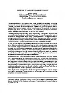
The following map (Figure 5) shows the final concentration map based on the self-adaptive The following map (Figure 5) shows the final concentration map based on the self-adaptive revised LURLUR model for for winter 2014 ininBeijing. withFigure Figure2,2, Figure 5 shows PM2.5 revised model winter 2014 Beijing.Compared Compared with Figure 5 shows highhigh PM2.5 concentrations in the southern regions low PM PM2.52.5concentrations concentrations in the north concentrations in the southern regionsofofBeijing Beijing and and low in the north and and northwestern regions of Beijing. northwestern regions of Beijing.

Figure 5. The distribution of PM 2.5 in the winter of 2014 in Beijing based on the self-adaptive revised Figure 5. The distribution of PM 2.5 in the winter of 2014 in Beijing based on the self-adaptive revised LUR model spatial interpolation. LUR model and and spatial interpolation.

4. Discussion of the Results

4. Discussion of the Results

In this section, we analyze the results from the three following aspects: accuracy analysis,

In this section, we typical analyze the results the threeanalysis following accuracy analysis, comparison with the LUR model, andfrom a characteristic of theaspects: PM2.5 concentrations for comparison with the typical LUR model, and a characteristic analysis of the PM Beijing in the winter of 2014. The reliability, superiority, and limitations of the self-adaptive revised for 2.5 concentrations Beijing in model the winter of 2014.inThe superiority, and limitations of the self-adaptive revised LUR are discussed thereliability, final portions of this section. LUR model are discussed in the final portions of this section. 4.1. Accuracy Analysis

4.1. Accuracy For Analysis the general LUR model, we use leave-one-out (LOO) cross-validation to evaluate the accuracy [34,41]. LOO N-1 sampling (herein the (LOO) monitoring sites) to train ortoconstruct a the For the general LURuses model, we usepoints leave-one-out cross-validation evaluate model and then uses the remaining true values observed at the sites to evaluate the accuracy of the accuracy [34,41]. LOO uses N-1 sampling points (herein the monitoring sites) to train or construct model prediction at a site. This procedure was repeated N times so that all sites were used as the a model and then uses the remaining true values observed at the sites to evaluate the accuracy of the evaluation site. However, the self-adaptive revised LUR model is a model group that combines the model prediction at a site. This procedure was repeated N times so that all sites were used as the general LUR model; thus, we use the accuracy of the final map to evaluate its stability. To obtain the evaluation site. However, the self-adaptive revised LUR model is a model group that combines the general LUR model; thus, we use the accuracy of the final map to evaluate its stability. To obtain the accuracy of the final map, we extracted the prediction values at the monitoring sites and compared them


16 of 23

with the true values. This analysis was carried out for the 35 monitoring sites based on the differences between the true values and the predicted values. Accuracy was determined using the following four evaluation methods: the mean error (ME), root-mean-square error (RMSE), standard deviation (SD), and mean error rate (MER). These accuracy metrics were computed using the following equations: N ř

εi ME “ i“1 N g fN fÿ RMSE “ e ε i 2 {N

(2)

(3)

i“1

g fN fÿ SD “ e pε i ´ MEq2 {N

(4)

i “1 N ř |ε|

MER “

i “1

Ti

ˆ 100% N

(5)

where ε i represents the difference between the true value and the predicted value for the ith predictor variable, N is the total number of true values involved in the accuracy analysis, and Ti is the true value of the ith variable. These four error evaluation methods have the following meanings. Smaller RMSEs correspond with higher accuracies. If the errors are distributed around the mean, the ME should be nearly zero. When the RMSE and SD are nearly the same, the accuracy is high. The MER reflects the proportion of the error relative to the true value, with smaller MERs indicating higher accuracy. In this paper, accuracy was evaluated from two perspectives. First, the accuracy was determined based on the PM2.5 concentration errors in the winter (as shown in Table 4 in Section 4.2, the general LUR model is evaluated based on the LOO validation and the accuracy of the final map). Second, a statistical analysis of the different monitoring sites (shown in Table 5 in Section 4.2) was conducted to determine the characteristics of the spatial variations in accuracy based on the self-adaptive and revised LUR models. As shown in Table 4 (comparison analysis), the total average error for winter based on the RMSE was 17.443 µg/m3 , and the SD was 17.395 µg/m3 , which is near the RMSE. In addition, the ME was 1.296 µg/m3 , which is nearly 0. Thus, the accuracy was sufficient. As shown in Table 5, the variations of the spatial accuracy based on the self-adaptive revised LUR models show specific characteristics. The traffic pollution monitoring sites had the lowest RMSEs and MERs, and the RMSEs and the SDs were nearly 0. Moreover, the MEs were nearly 0. Thus, the prediction model (self-adaptive revised LUR model) had the highest accuracy for the traffic pollution monitoring sites. In addition, the suburban environmental evaluation sites and the regional background control sites exhibited lower accuracy than the urban environmental evaluation sites and the traffic pollution monitoring sites. As shown in Figure 1, the urban environmental evaluation sites and traffic pollution monitoring sites are located around the city center, and suburban pollution monitoring and regional background control sites are located in the suburbs. Thus, the self-adaptive revised LUR model was more accurate near the center of Beijing than in the suburbs. 4.2. Comparison with the Typical LUR Method We also compared the self-adaptive and revised methods using the typical LUR model from the following two aspects: SPER and accuracy.


(1)

17 of 23

SPER

One of the most obvious advantages of the self-adaptive revised LUR model is its ability to improve the SPER relative to the typical LUR model. The SPER of the typical LUR model for the winter of 2014 in Beijing is 75%, while our method improves it to 90%. (2)

Accuracy

In this study, the typical LUR model and the self-adaptive revised LUR model were constructed using the same predictor variables. Then, we compared the ME, RMSE, SD, and ME for the self-adaptive LUR model and the typical LUR model using the final map accuracy with LOO cross-validation to evaluate the accuracy. The results are shown in Table 4. In addition, we compared the accuracies of the different monitoring sites (by evaluating the accuracy of the final map) to determine the spatial variation of the accuracy (shown in Table 5). Table 4. Accuracy of the PM2.5 estimations based on four metrics for Beijing in 2014. Error

ME (µg/m3 )

RMSE (µg/m3 )

SD (µg/m3 )

MER (%)

Self-adaptive LUR models (Final map accuracy) Typical model (Final map accuracy) Typical model (LOO cross validation)

1.296 9.982 1.438

17.443 20.643 24.7389

17.395 18.069 24.6971

14.658 19.488 21.365

Table 5. Accuracies of PM2.5 estimations at the different monitoring sites in Beijing in 2014. Monitoring Sites in the Different Regions

ME (µg/m3 )

RMSE (µg/m3 )

SD (µg/m3 )

MER (%)

Urban environmental evaluation site

Self-adaptive LUR models Typical model

0.768 13.414

11.897 17.546

11.873 11.311

10.598 17.147

Suburban environmental evaluation site


5.070 12.600

18.748 19.792

18.050 15.263

17.475 20.369

Regional background control site


1.243 ´2.112

25.946 28.639

25.916 28.561

23.004 26.371

Traffic pollution monitoring site


´5.666 12.914

8.629 15.298

6.508 8.201

6.526 13.535

According to Table 4, the ME, RMSE, SD, and MER computed from the self-adaptive LUR models were all smaller than those computed using the typical LUR model based on both final map accuracy and LOO cross-validation. Specifically, the ME was closer to 0, the predicted values all changed around the true value, and the RMSE and MER were small, which indicated higher accuracy. Moreover, the RMSE was closer to the SD for the self-adaptive LUR model than the typical model, which also indicated higher accuracy. Generally, the accuracy of the PM2.5 concentrations was computed using the self-adaptive LUR model and was higher than the typical LUR model. In addition, the accuracy of the typical LUR model evaluated using LOO cross validation (result before Kriging interpolation) was less than the final map accuracy, which verified that Kriging improves the accuracy of the LUR model [50]. According to Table 5, the MEs, RMSEs, SDs, and MERs were all small when computed using the self-adaptive revised LUR model than the typical model. For the suburban environmental evaluation sites, the self-adaptive revised LUR model and the typical model exhibited similar accuracies. Generally, the self-adaptive revised LUR model improved the accuracy of the typical LUR model. 4.3. Spatial Variations of the PM2.5 Concentrations We also analyzed the spatial distribution characteristics of PM2.5 in Beijing during the winter. To make this analysis more intuitive, we drew a line from north to south that successively crossed the different ring roads in Beijing as well as the center of Beijing, which is the brown line shown in

Sustainability2016, 2016,8,8,786 786 Sustainability

18ofof23 23 18

To make make this this analysis analysis more more intuitive, intuitive, we we drew drewaa line line from from north north toto south south that that successively successively To 18 of 23 crossed the different ring roads in Beijing as well as the center of Beijing, which is the brown line crossed the different ring roads in Beijing as well as the center of Beijing, which is the brown line shownininFigure Figure6.6.In Inaddition, addition,we weextracted extractedthe thePM PM2.52.5concentrations concentrationsfor forthe thearea areadenoted denotedininFigure Figure shown 6, which are also shown in Figure 7, to analyze changes in the PM 2.5concentrations concentrations in the different 6, which are also shown in Figure 7, to analyze changes in the PM 2.5 in the different Figure 6. In addition, we extracted the PM2.5 concentrations for the area denoted in Figure 6, which regions. regions. are also shown in Figure 7, to analyze changes in the PM2.5 concentrations in the different regions.


Figure6.6.Profile Profileline linefrom fromnorth northtotosouth southininBeijing. Beijing. Figure

Figure PM concentration variation profile for winter 2014 in Beijing. 2.5 Figure7. PM 2.5concentration concentrationvariation variationprofile profilefor forwinter winter2014 2014in inBeijing. Beijing. Figure 7.7.PM 2.5

According to Figure spatialdistribution distributioncharacteristics characteristics can summarized as follows. Accordingto toFigure Figure5,5,the thespatial spatial distribution characteristics can bebe summarized asfollows. follows. (1) can be summarized as (1) (1) The PM concentrations in the region southeast of Beijing were generally higher than those in The PM 2.5concentrations concentrations the region southeast ofBeijing Beijing were generally higher than those the The PM 2.5 ininthe region southeast of were generally higher than those ininthe 2.5 the northwest; The most seriously polluted areas Beijingin inthe thewinter winterwere werethe the Tongzhou northwest; (2)(2) The most seriously polluted areas Beijing in the winter theTongzhou Tongzhouand and northwest; (2) The most seriously polluted areas ininin Beijing Daxing DaxingDistricts, Districts,the thesouthwest southwestregion regionofofthe theFangshan FangshanDistrict, District,Miyun MiyunCounty Countyand andits itssurrounding surrounding area, region ofof Yanqing County, the the southern region of the Pinggu District, and the south area,the thesouthwest southwest region ofYanqing Yanqing County, thesouthern southern region of thePinggu Pinggu District, and the area, the southwest region County, region of the District, and the regions of the Shunyi, Chaoyang, and Dongcheng Districts. Districts. To analyze the characteristics of the spatial southregions regions ofthe theShunyi, Shunyi,Chaoyang, Chaoyang, andDongcheng Dongcheng Districts. To analyze thecharacteristics characteristics south of and To analyze the ofof variation of PM2.5 in Beijing, we analyzed the PM2.5 concentration profile (Figure 7). Figure 7 shows that the spatial distribution of PM2.5 in Beijing varied from north to south as follows: (1) the PM2.5


19 of 23

concentration generally increased from north to south, validating the first characteristic discussed above; and (2) the highest PM2.5 concentration during the winter was observed from the south fourth ring road to the southern suburban area and the lowest PM2.5 concentration during the winter was found in the northern suburban area. Overall, the spatial distribution of PM2.5 in Beijing in 2014 exhibited the following main characteristics: the PM2.5 concentrations were low in the north, particularly in the northwest, and were high in the central and southern regions. 4.4. Reliability, Superiority, and Limitations of the Revised LUR Model and Future Research Reliability of the self-adaptive revised LUR model: The accuracy analysis showed that the overall accuracy is satisfactory, and the analysis of spatial variations in accuracy showed that the accuracy was highest near the city center, which is consistent with the fact that the monitoring sites are concentrated in central Beijing. The spatial variation analysis showed that the PM2.5 concentrations were low to the north, particularly in the northwest region of Beijing, and high in the southern and central regions of Beijing. The spatial variation analysis results were consistent with the fact that the northern region of Beijing is mountainous and contains few people; thus, less transportation is used in this region than in other regions, resulting in reduced pollutant concentrations. In the central region, a high population density and heavy traffic resulted in high pollution levels. Furthermore, the area south and southwest of Beijing, which is adjacent to Hebei province, contains many polluting enterprises. Consequently, high PM2.5 concentrations were found in this region. Therefore, the results are consistent and show the reliability of the self-adaptive revised LUR model. An error distribution map is shown in Figure 8, which is consistent with the results that suburban environmental evaluation sites have low accuracies in Section 4.1. The spatial autocorrelated analysis also showed the errors are not autocorrelated, which increased the reliability of this model. (2) Superiority of the self-adaptive LUR model: The SPER of the self-adaptive LUR model relative to the typical LUR model increased from 75% to 90%. In addition, the accuracy increased with RMSE from 20.643 µg/m3 to 17.443 µg/m3 . Meanwhile, the adjusted R-squared value for the general LUR model was 0.679, and the adjusted R-squared values for the self-adaptive LUR models for the out-of-range sampling points were more than 0.5. Hence, the self-adaptive revised LUR model was superior to the typical LUR model. (3) Limitations of the self-adaptive LUR model: When the typical LUR model does not result in an SPER of at least 80%, or when negative values are observed in the prediction results, the self-adaptive revised LUR model can be used for improving the SPER and accuracy. If the SPER is at least 90%, the self-adaptive LUR model will not improve the accuracy of the typical LUR model. Thus, if the explanation ability of the model is high and we want to improve the accuracy, the best predictor variables should be chosen because previous studies have indicated that more comprehensive predictor variables result in more accurate final LUR models. (4) Future work: The effectiveness of the self-adaptive revised LUR model for estimating the PM2.5 concentrations for winter 2014 in Beijing is shown in this study. The presented approach will be effective for estimating the concentrations of other pollutants and other periods (e.g., spring, summer, and autumn of a year) in the future. Furthermore, this method can be used at high spatial scales, such as the national scale, because more sampled points will be outside of the data range, and the self-adaptive revised LUR model will be more effective. However, we used several open-sourced predictor variables. Thus, if possible, more predictor variables (i.e., meteorological data) should be used in future studies.

(1)

which is adjacent to Hebei province, contains many polluting enterprises. Consequently, high PM2.5 concentrations were found in this region. Therefore, the results are consistent and show the reliability of the self-adaptive revised LUR model. An error distribution map is shown in Figure 8, which is consistent with the results that suburban environmental evaluation sites have low accuracies not Sustainability 2016, 8, 786 in Section 4.1. The spatial autocorrelated analysis also showed the errors are 20 of 23 autocorrelated, which increased the reliability of this model.

Figure 8. The error distribution map of the self-adaptive revised LUR model at different monitoring Figure 8. The error distribution map of the self-adaptive revised LUR model at different monitoring sites. Circles of the same size but with different colors represent different error ranges. sites. Circles of the same size but with different colors represent different error ranges.

5. (2) Conclusions Superiority of the self-adaptive LUR model: The SPER of the self-adaptive LUR model relative to the typicalwith LURprevious model increased to 90%. In addition, accuracyofincreased with Compared studies,from we 75% aimed to improve the the accuracy LUR model. Thus, we introduced a novel approach for estimating PM2.5 concentrations in this paper (i.e., a self-adaptive revised LUR model). The developed self-adaptive revised LUR model combines the typical LUR model and the self-adaptive LUR model group. The typical LUR model was used as a general model for predicting the sampled points in the target area. The self-adaptive LUR model group was used to remove sampled points that did not satisfy the concentration range. Moreover, the self-adaptive LUR model (a regression model) is adaptive to its own independent variables, which are nonzero for each sample point. The self-adaptive LUR model is a real-time model and may provide different results for each sample point. The self-adaptive LUR model group is only suitable for sampled points that are removed by the typical LUR model because of negative or out-of-range values. The PM2.5 concentrations were estimated for winter 2014 to illustrate the model. Both the typical and self-adaptive revised LUR models were used. The results were discussed, and the reliability and superiority of the self-adaptive revised LUR model were shown. The self-adaptive, revised LUR model can improve the accuracy of air pollution distributions. The results of this investigation demonstrate that such enhancements can contribute to the tools needed to predict future scenarios, which is an important part of pollution prevention and sustainable solutions. Thus more effective measures for air pollution can be realized based on different methods for different level of air pollution in different districts, or villages. For example, we can analyze the specific reason for different level of air pollution though the way of overlaying the air pollution distribution maps with the other thematic maps. e.g., if the accurate PM2.5 distribution map is overlaid with a road map, then we can find out whether the area with high road density has a high level of air pollution; if the accurate PM2.5 distribution map is overlaid with a land use map, we can see which type of land use has higher air pollution and which has less, and the measures can be made for the high air pollution areas with less forest land through planting more trees. Moreover, with the highest and the lowest rank of the air pollution for different districts of a city, which were obtained from the air pollution distribution map, the government can advocate for effective measures from regions with less air pollution. In short, a novel, effective way to achieve accurate distribution of PM2.5 air pollution is an analysis base for preventing air pollution and improving environmental sustainability.


21 of 23

Acknowledgments: This work was supported by the Fundamental Research Funds for the Central Universities, No. 2014205020203, and Special Funds Scientific Research Projects in Public Welfare Industry for Surveying and Mapping Geographic Information, No. 201512032. Assistant Qiu and Researcher Tao provided many suggestions and carefully reviewed the article; we express our appreciation for their significant contributions to this article. Author Contributions: Lujin Hu conceived and designed the self-adaptive revised LUR model and performed the main portions of the experiment. Jiping Liu and Zongyi He provided advice regarding the self-adaptive revised LUR model method and performed part of the experimental analysis. Conflicts of Interest: The authors declare no conflict of interest.

References 1.

2. 3.

4. 5. 6.

7. 8. 9. 10.

11.

12.

13.

14. 15.

Air Quality Expert Group to the Department for Environment. Fine Particulate Matter (PM2.5 ) in the United Kingdom. Available online: http://UKair.defra.gov.UK/assets/documents/reports/cat11/1212141150_ AQEG_Fine_Particulate_Matter_in_the_UK.pdf (accessed on 25 November 2015). Martinelli, N.; Olivieri, O.; Girelli, D. Air particulate matter and cardiovascular disease: A narrative review. Eur. J. Intern. Med. 2013, 24, 295–302. [CrossRef] [PubMed] Fantke, P.; Jolliet, O.; Evans, J.S.; Apte, J.S.; Cohen, A.J.; Hanninen, O.O.; Hurley, F.; Jantunen, M.J.; Jerrett, M.; Levy, J.I.; et al. Health effects of fine particulate matter in life cycle impact assessment: Findings from the Basel Guidance Workshop. Int. J. Life Cycle Assess. 2015, 20, 276–288. [CrossRef] LUKe, C.; Rea, W.; Smith-Willis, P.; Fenyves, E.; Pan, Y. Adverse health effects of outdoor air pollutants. Environ. Int. 2006, 32, 815–830. Giorginia, P.; Di Giosia, P.; Grassi, D.; Rubenfire, M.; Brook, R.D.; Ferri, C. Air pollution exposure and blood pressure: An updated review of the literature. Curr. Pharm. Des. 2016, 22, 28–51. [CrossRef] Wang, M.; Gehring, U.; Hoek, G.; KeUKen, M.; Jonkers, S.; Beelen, R.; Eeftens, M.; Postma, D.S.; Brunekreef, B. Air pollution and lung function in dutch children: A comparison of exposure estimates and associations based on land use regression and dispersion exposure modeling approaches. Environ. Health Perspect. 2015, 123, 847–851. [CrossRef] [PubMed] Madaniyazi, L.; Nagashima, T.; Guo, Y.M.; Yu, W.W.; Tong, S.L. Projecting fine particulate matter-related mortality in east China. Environ. Sci. Technol. 2015, 49, 11141–11150. [CrossRef] [PubMed] Dugord, P.A.; Lauf, S.; Schuster, C.; Kleinschmit, B. Land use patterns, temperature distribution, and potential heat stress risk—The case study Berlin, Germany. Comput. Environ. Urban Syst. 2014, 48, 86–98. [CrossRef] Ito, K.; Kinney, P.L.; Thurston, G.D. Variations in PM10 concentrations within 2 metropolitan-areas and their implications for health-effects analyses. Inhal. Toxicol. 1995, 7, 735–745. [CrossRef] Hoek, G.; Krishnan, R.M.; Beelen, R.; Peters, A.; Ostro, B.; Brunekreef, B.; Kaufman, J.D. Long-term air pollution exposure and cardio- respiratory mortality: A review. Environ. Health 2013, 12. [CrossRef] [PubMed] Beelen, R.; Hoek, G.; Raaschou-Nielsen, O.; Stafoggia, M.; Andersen, Z.J.; Weinmayr, G.; Hoffmann, B.; Wolf, K.; Samoli, E.; Fischer, P.H.; et al. Natural-cause mortality and long-term exposure to particle components: An analysis of 19 European cohorts within the multi-center ESCAPE project. Environ. Health Perspect. 2015, 123, 525–533. [CrossRef] [PubMed] Beelen, R.; Hoek, G.; Vienneau, D.; Eeftens, M.; Dimakopoulou, K.; Pedeli, X.; Tsai, M.Y.; Kunzli, N.; Schikowski, T.; Marcon, A.; et al. Development of NO2 and NOx land use regression models for estimating air pollution exposure in 36 study areas in Europe—The ESCAPE project. Atmos. Environ. 2013, 72, 10–23. [CrossRef] Ross, Z.; Ito, K.; Johnson, S.; Yee, M.; Pezeshki, G.; Clougherty, J.E.; Savitz, D.; Matte, T. Spatial and temporal estimation of air pollutants in New York City: Exposure assignment for use in a birth outcomes study. Environ. Health 2013, 12. [CrossRef] [PubMed] Wu, J.; Wilhelm, M.; Chung, J.; Ritz, B. Comparing exposure assessment methods for traffic-related air pollution in an adverse pregnancy outcome study. Environ. Res. 2011, 111, 685–692. [CrossRef] [PubMed] Lakshmanan, A.; Chiu, Y.H.M.; Coull, B.A.; Just, A.C.; Maxwell, S.L.; Schwartz, J.; GryParis, A.; Kloog, I.; Wright, R.J.; Wright, R.O. Associations between prenatal traffic-related air pollution exposure and birth weight: Modification by sex and maternal pre-pregnancy body mass index. Environ. Res. 2015, 137, 268–277. [CrossRef] [PubMed]


16. 17. 18. 19.

20.

21.

22.

23. 24.

25.

26.

27. 28.

29.

30.

31.

32.

33.

34.

22 of 23

Nieuwenhuijsen, M.J.; Basagana, X.; Dadvand, P.; Martinez, D.; Cirach, M.; Beelen, R.; Jacquemin, B. Air pollution and human fertility rates. Environ. Int. 2014, 70, 9–14. [CrossRef] [PubMed] Krstic, G. A reanalysis of fine particulate matter air pollution versus life expectancy in the United States. J. Air Waste Manag. Assoc. 2013, 63, 133–135. [CrossRef] [PubMed] Pope, C.A., III; Ezzati, M.; Dockery, D.W. Fine particulate air pollution and life expectancies in the United States: The role of influential observations. J. Air Waste Manag. Assoc. 2013, 63, 129–132. [CrossRef] [PubMed] Cohen, A.J.; Anderson, H.R.; Ostro, B.; Pandey, K.D.; Krzyzanowski, M.; Kunzli, N.; Gutschmidt, K.; Pope, A.; Romieu, I.; Samet, J.M.; et al. The global burden of disease due to outdoor air pollution. J. Toxicol. Environ. Health A 2005, 68, 1301–1307. [CrossRef] [PubMed] Mehta, S.; Shin, H.; Burnett, R.; North, T.; Cohen, A.J. Ambient particulate air pollution and acute lower respiratory infections: A systematic review and implications for estimating the global burden of disease. Air Qual. Atmos. Health 2013, 6, 69–83. [CrossRef] [PubMed] WHO Press (2006) WHO Air Quality Guidelines for Particulate Matter, Ozone, Nitrogen Dioxide and Sulfur Dioxide. World Health Organization. Available online: http://whqlibdoc.who.int/hq/2006/WHO_SDE_ PHE_OEH_06.02_eng.pdf (accessed on 25 October 2014). Restrictions Announcement of Traffic Management Measures of Beijing Municipal People’s Government on Weekday Peak Areas. Available online: http://zhengwu.Beijing.gov.cn/gzdt/gggs/t1430212.htm (accessed on 5 October 2015). Air Quality of Beijing. Available online: http://zx.bjmemc.com.cn/ (accessed on 5 October 2015). Beckerman, B.S.; Jerrett, M.; Serre, M.; Martin, R.V.; Lee, S.J.; van Donkelaar, A.; Ross, Z.; Su, J.; Burnett, R.T. A hybrid approach to estimating national scale spatiotemporal variability of PM2.5 in the contiguous United States. Environ. Sci. Technol. 2013, 47, 7233–7241. [PubMed] Briggs, D.J.; Collins, S.; Elliott, P.; Fischer, P.; Kingham, S.; Lebret, E.; Pryl, K.; Van Reeuwijk, H.; Smallbone, K.; Van Der Veen, A. Mapping urban air pollution using GIS: A regression-based approach. Int. J. Geogr. Inf. Sci. 1997, 11, 699–718. [CrossRef] Aguilera, I.; Eeftens, M.; Meier, R.; Ducret-Stich, R.E.; Schindler, C.; Ineichen, A.; Phuleria, H.C.; Probst-Hensch, N.; Tsai, M.Y.; Kunzli, N. Land use regression models for crustal and traffic-related PM2.5 constituents in four areas of the SAPALDIA study. Environ. Res. 2015, 140, 377–384. [CrossRef] [PubMed] Reyes, J.M.; Serre, M.L. An LUR/BME framework to estimate PM2.5 explained by on road mobile and stationary sources. Environ. Sci. Technol. 2014, 48, 1736–1744. [CrossRef] [PubMed] Wu, C.F.; Lin, H.I.; Ho, C.C.; Yang, T.H.; Chen, C.C.; Chan, C.C. Modeling horizontal and vertical variation in intraurban exposure to PM2.5 concentrations and compositions. Environ. Res. 2014, 133, 96–102. [CrossRef] [PubMed] Chen, C.C.; Wu, C.F.; Yu, H.L.; Chan, C.C.; Cheng, T.J. Spatiotemporal modeling with temporal-invariant variogram subgroups to estimate fine particulate matter PM2.5 concentrations. Atmos. Environ. 2012, 54, 1–8. [CrossRef] Hankey, S.; Marshall, J.D. Land use regression models of on-road particulate air pollution (particle number, black carbon, PM2.5 , particle size) using mobile monitoring. Environ. Sci. Technol. 2015, 49, 9194–9202. [CrossRef] [PubMed] Saraswat, A.; Apte, J.S.; Kandlikar, M.; Brauer, M.; Henderson, S.B.; Marshall, J.D. Spatiotemporal land use regression models of fine, ultrafine, and black carbon particulate matter in New Delhi, India. Environ. Sci. Technol. 2013, 47, 12903–12911. [CrossRef] [PubMed] Wang, M.; Beelen, R.; Basagana, X.; Becker, T.; Cesaroni, G.; de Hoogh, K.; Dedele, A.; Declercq, C.; Dimakopoulou, K.; Eeftens, M.; et al. Evaluation of land use regression models for NO2 and particulate matter in 20 European study areas: The ESCAPE project. Environ. Sci. Technol. 2013, 47, 4357–4364. [CrossRef] [PubMed] Vienneau, D.; de Hoogh, K.; Bechle, M.J.; Beelen, R.; van Donkelaar, A.; Martin, R.V.; Millet, D.B.; Hoek, G.; Marshall, J.D. Western European land use regression incorporating satellite- and ground-based measurements of NO2 and PM10 . Environ. Sci. Technol. 2013, 47, 13555–13564. [CrossRef] [PubMed] Liu, W.; Li, X.D.; Chen, Z.; Zeng, G.M.; Leon, T.; Liang, J.; Huang, G.H.; Gao, Z.H.; Jiao, S.; He, X.X.; et al. Land use regression models coupled with meteorology to model spatial and temporal variability of NO2 and PM10 in Changsha, China. Atmos. Environ. 2015, 116, 272–280. [CrossRef]


35.

36.

37.

38.

39.

40. 41. 42.

43.

44. 45. 46. 47. 48. 49. 50.

23 of 23

Kerckhoffs, J.; Wang, M.; Meliefste, K.; Malmqvist, E.; Fischer, P.; Janssen, N.A.H.; Beelen, R.; Hoek, G. A national fine spatial scale land-use regression model for ozone. Environ. Res. 2015, 140, 440–448. [CrossRef] [PubMed] Molter, A.; Lindley, S.; de Vocht, F.; Simpson, A.; Agius, R. Modelling air pollution for epidemiologic research—Part i: A novel approach combining land use regression and air dispersion. Sci. Total Environ. 2010, 408, 5862–5869. [CrossRef] [PubMed] De Hoogh, K.; Korek, M.; Vienneau, D.; Keuken, M.; Kukkonen, J.; Nieuwenhuijsen, M.J.; Badaloni, C.; Beelen, R.; Bolignano, A.; Cesaroni, G.; et al. Comparing land use regression and dispersion modelling to assess residential exposure to ambient air pollution for epidemiological studies. Environ. Int. 2014, 73, 382–392. [CrossRef] [PubMed] Yu, H.L.; Wang, C.H.; Liu, M.C.; Kuo, Y.M. Estimation of fine particulate matter in Taipei using landuse regression and bayesian maximum entropy methods. Int. J. Environ. Res. Public Health 2011, 8, 2153–2169. [CrossRef] [PubMed] Fischer, P.H.; Marra, M.; Ameling, C.B.; Hoek, G.; Beelen, R.; de Hoogh, K.; Breugelmans, O.; Kruize, H.; Janssen, N.A.H.; Houthuijs, D. Air pollution and mortality in seven million adults: The dutch environmental longitudinal study (DUELS). Environ. Health Perspect. 2015, 123, 697–704. [CrossRef] [PubMed] Ryan, P.H.; LeMasters, G.K. A review of land-use regression for characterizing intraurban air models pollution exposure. Inhal. Toxicol. 2007, 19, 127–133. [CrossRef] [PubMed] Wu, J.S.; Li, J.C.; Peng, J.; Li, W.F.; Xu, G.; Dong, C.C. Applying land use regression model to estimate spatial variation of PM2.5 in Beijing, China. Environ. Sci. Pollut. Res. 2015, 22, 7045–7061. [CrossRef] [PubMed] Lee, J.H.; Wu, C.F.; Hoek, G.; de Hoogh, K.; Beelen, R.; Brunekreef, B.; Chan, C.C. Lur models for particulate matters in the Taipei metropolis with high densities of roads and strong activities of industry, commerce and construction. Sci. Total Environ. 2015, 514, 178–184. [CrossRef] [PubMed] Carter, E.M.; Shan, M.; Yang, X.D.; Li, J.R.; Baumgartner, J. Pollutant emissions and energy efficiency of Chinese gasifier cooking stoves and implications for future intervention studies. Environ. Sci. Technol. 2014, 48, 6461–6467. [CrossRef] [PubMed] National Bureau of Technical Supervision of the People’s Republic of China, GB3095-2012. Ambient Air Quality Standards; Chinese Standard Press: Beijing, China, 2013. National Bureau of Technical Supervision of the People’s Republic of China, HJ633-2012. Technical Regulation on Ambient Air Quality Index (on Trial); Chinese Standard Press: Beijing, China, 2013. National Bureau of Technical Supervision of the People’s Republic of China, 21010-2007, G.T. Current Land Use Classification Standard; Chinese Standard Press: Beijing, China, 2007. Openstreetmap Geofabrik Downloads. Available online: http://download.geofabrik.de/ (accessed on 5 October 2015). Beijing statistics Bureau. Beijing Statistical Yearbook of 2014; China Statistic Press: Beijing, China, 2014. Points of Interest SWG. Available online: http://www.opengeospatial.org/projects/groups/poiswg (accessed on 15 May 2016). Zou, B.; Luo, Y.Q.; Wan, N.; Zheng, Z.; Sternberg, T.; Liao, Y.L. Performance comparison of LUR and OK in PM2.5 concentration mapping: A multidimensional perspective. Sci. Rep. 2015, 5. [CrossRef] [PubMed] © 2016 by the authors; licensee MDPI, Basel, Switzerland. This article is an open access article distributed under the terms and conditions of the Creative Commons Attribution (CC-BY) license (http://creativecommons.org/licenses/by/4.0/).

Self-Adaptive Revised Land Use Regression Models for ... - MDPI

Self-Adaptive Revised Land Use Regression Models for ... - MDPI

Suggest Documents

Development of land use regression models for nitrogen dioxide ...

Development of temporally refined land-use regression models ...

Land Use Regression Modeling of PM2.5 Concentrations at ... - MDPI

Land Use Regression Modeling of Outdoor Noise Exposure in ... - MDPI

Comparison of Land-Use Regression Modeling with ... - MDPI

Use of Pollutant Load Regression Models with Various ... - MDPI

Integrating Address Geocoding, Land Use Regression, and ...

Comparing land use regression and dispersion ...

Concurrent Spatiotemporal Daily Land Use Regression ... - bioRxiv

A Land Use Regression Model for Predicting Ambient Concentrations ...

Development of Land Use Regression Models for PM2. 5, PM2. 5 ...

Empirical Regression Models for Estimating Multiyear Leaf ... - MDPI

Agent-based land-use models - Core

overview of land-use transport models - CiteSeerX

Current and Future Land Use Models - CiteSeerX

OVERVIEW OF LAND-USE TRANSPORT MODELS

INTEGRATED BIO-ECONOMIC LAND USE MODELS

DIAGNOSTIC TECHNIQUES FOR REGRESSION MODELS

Integrative Assessment of Land Use Conflicts - MDPI

Scenario-Based Simulation on Dynamics of Land-Use-Land ... - MDPI

Integrating Biophysical and Socio-Economic Models for Land Use ...

Walkability, Land Use and Physical Activity - MDPI

Comparison of regression models with land-use and emission data to ...

Comparison of regression models with land-use and emission data to ...