Self-avoiding walk on nonunimodular transitive graphs

Self-avoiding walk on nonunimodular transitive graphs

arXiv:1709.10515v1 [math.PR] 29 Sep 2017

Tom Hutchcroft∗ October 2, 2017

Abstract We study self-avoiding walk on graphs whose automorphism group has a transitive nonunimodular subgroup. We prove that self-avoiding walk is ballistic, that the bubble diagram converges at criticality, and that the critical two-point function decays exponentially in the distance from the origin. This implies that the critical exponent governing the susceptibility takes its mean-field value, and hence that the number of self-avoiding walks of length n is comparable to the nth power of the connective constant. We also prove that the same results hold for a large class of repulsive walk models with a self-intersection based interaction, including the weakly self-avoiding walk. All these results apply in particular to the product Tk × Zd of a k-regular tree (k ≥ 3) with Zd , for which these results were previously only known for large k.

1

Introduction

A self-avoiding walk (SAW) on a graph G is a path in G that visits each vertex at most once. In the probabilistic study of self-avoiding walk, one fixes a graph (often the hypercubic lattice Zd ), and is interested in both enumerating the number of n-step SAWs and studying the asymptotic behaviour of a uniformly random SAW of length n. This leads to two particularly important questions. Question 1.1. What is the asymptotic rate of growth of the number of SAWs of length n? Question 1.2. How far from the origin is the endpoint of a typical SAW of length n? These questions are simple to state but are often very difficult to answer. Substantial progress has been and continues to be made for SAW on Euclidean lattices. In particular, a very thorough understanding of SAW on Zd for d ≥ 5 has been established in the seminal work of Hara and Slade [24, 23]. The low-dimensional cases d = 2, 3, 4 continue to present serious challenges. For a comprehensive introduction to and overview of this literature, we refer the reader to [31, 2]. Recently, the study of SAW on more general graphs has gathered momentum. In particular, a systematic study of SAW on transitive graphs has been initiated in a series of papers by Grimmett and Li [11, 17, 13, 16, 18, 14, 15], which is primarily concerned with properties of the connective constant. Other works on SAW on non-Euclidean transitive graphs include [12, 33, 3, 29, 32, 10]. See [19] for a survey of these results. ∗

Statistical Laboratory, DPMMS, Univeristy of Cambridge, and Trinity College, Cambridge.

1

In this paper, we given complete answers to Question 1.1 and Question 1.2 for self-avoiding walk on graphs whose automorphism group admits a nonunimodular transitive subgroup (defined in the next subsection). Although graphs whose entire automorphism group is nonunimodular are generally considered to be rather contrived and unnatural, the class of graphs with a nonunimodular transitive subgroup of automorphisms is much larger. Indeed, it includes natural examples such as the product Tk × Zd of a k-regular tree with Zd for every k ≥ 3 (or indeed Tk × H where H is an arbitrary transitive graph), for which the results of this paper were only previously known for large values of k (see the discussion at the end of this subsection). Our proofs are inspired by the analysis we carried out for percolation on the same class of graphs in our forthcoming paper [25], which relies on similar methodology. It should be remarked that although every graph possessing a transitive nonunimodular subgroup of automorphisms is necessarily nonamenable [36], we never use this fact in our analysis. Our first theorem answers Question 1.1 in the nonunimodular context. Let G be a transitive graph, let 0 be a fixed root vertex of G, and let Z(n) be the number of length n SAWs in G starting at 0. Hammersley and Morton [20] observed that Z(n) satisfies the submultiplicative inequality Z(n + m) ≤ Z(n)Z(m), from which it follows by Fekete’s Lemma that there exists a constant µc = µc (G), known as the connective constant of G, such that µc = lim Z(n)1/n = inf Z(n)1/n , n→∞

n≥1

so that in particular µnc ≤ Z(n) ≤ µn+o(n) c for every n ≥ 0. We also define the susceptibility χ(z) to be the generating function χ(z) =

X

z n Z(n),

n≥0

which has radius of convergence zc := µ−1 c . The connective constant is not typically expected to have a nice or interesting value (a notable exception is the hexagonal lattice [34, 9]), and it is typically much more interesting to estimate the subexponential correction to Z(n) than it is to estimate µc . We stress that submultiplicativity arguments alone do not yield any control of this subexponential correction whatsoever. Theorem 1.3 (Counting walks). Let G be a connected, locally finite graph, and suppose that Aut(G) has a transitive nonunimodular subgroup. Then there exists a constant C such that Czc zc ≤ χ(z) ≤ zc − z zc − z

and

µnc ≤ Z(n) ≤ Cµnc

for every 0 ≤ z < zc and n ≥ 0. In fact we are able to obtain explicit estimates on the constants that appear in this theorem, see Remark 3.5. The lower bounds of the theorem are trivial consequences of submultiplicativity. The upper bounds on χ(z) and Z(n) in this theorem are equivalent up to the choice of constant, 2

see Lemma 3.4. Probabilistically, the upper bound on Z(n) means that the concatenation of two uniformly chosen n-step SAWs has probability at least 1/C > 0 to be self-avoiding for every n ≥ 0. Our next theorem answers Question 1.2 in the nonunimodular context. We define Pn to be the uniform measure on self-avoiding walks of length n in G starting at 0, and denote the random self-avoiding walk sampled from Pn by X = (Xi )ni=0 . For each z ≥ 0 and x ∈ V , we define the two-point function G(z; x) =

X

ω∈Ω


X n z |ω| 1 ω : 0 → x self-avoiding = z Z(n)Pn (Xn = x) . n≥0

In the following theorem, d(0, x) denotes the graph distance between 0 and x. Theorem 1.4 (Speed and two-point function decay). Let G = (V, E) be a connected, locally finite graph, and suppose that Aut(G) has a transitive nonunimodular subgroup. Then there exists a positive constant c such that   G(zc ; x) ≤ exp −cd(0, x) for every x ∈ V and

for every n ≥ 0.


Pn d(0, Xn ) ≥ cn ≥ 1 − exp [−cn]

Let us briefly survey related theorems in the literature. It is reasonable to conjecture that the conclusions of Theorems 1.3 and 1.4 hold for every transitive nonamenable graph. Indeed, it is plausible that the conclusion of Theorem 1.3 holds for every transitive graph with at least quintic volume growth. The conjectures are trivial when the graph is a tree. Li [29] has shown that SAW is ballistic on any infinitely ended transitive graph, and Madras and Wu [32] and Benjamini [3] have shown that SAW on certain specific hyperbolic lattices has linear mean displacement. Gilch and M¨ uller [10] have proven that the conclusions of Theorem 1.3 hold for free products of quasitransitive graphs (which are always infinitely ended), and Madras and Wu [32] have shown that they hold for certain hyperbolic lattices. Nachmias and Peres [33] proved that the conclusions of Theorems 1.3 and 1.4 hold for every transitive nonamenable graph satisfying (d − 1)ρ < µc ,

(1.1)

where d is the degree of the graph, ρ is its spectral radius, and µc is its connective constant. In particular, this holds whenever ρ ≤ 1/2 [35], as well as for nonamenable transitive graphs of large girth (where what constitutes ‘large’ depends on the spectral radius and the degree). However, it is possible to show that the criterion does does not apply to Tk × Zd unless k is reasonably large. For the hypercubic lattice, Hara and Slade [24, 23] proved that Z(n) grows like µnc as n → ∞ whenever d ≥ 5. In the same setting, they also proved that the distance from the origin to the endpoint of an n-step SAW is typically of order n1/2 . Hara [22] later proved that the critical twopoint function decays like kxk−d+2 . (Both behaviours are the same as for simple random walk). For d = 4 it is conjectured that similar asymptotics hold up to logarithmic corrections. See [1] and references therein for an account of substantial recent progress on four dimensional weakly 3

self-avoiding walk. For d = 2, 3 the gap between what is known and what is conjectured is very large; important results include those of [21, 28, 8, 7]. See [2, 31] and references therein for more details.

1.1

Tilted walks and the modular function

We now define unimodularity and nonunimodularity. Let G = (V, E) be a connected, locally finite graph, and let Aut(G) be the group of automorphisms of G. Recall that a subgroup Γ ⊆ Aut(G) is said to be transitive if it acts transitively on G, that is, if for any two vertices u, v ∈ V there exists γ ∈ Γ such that γu = v. The modular function ∆ = ∆Γ : V 2 → (0, ∞) of a transitive subgroup Γ ⊆ Aut(G) is defined to be ∆(x, y) =

| Staby x| , | Stabx y|

where Stabx y is the orbit of y under the stabilizer of x in Γ. The group Γ is said to be unimodular if ∆ ≡ 1, and nonunimodular otherwise. The most important properties of the modular function are the cocycle identity, which states that ∆(x, y)∆(y, z) = ∆(x, z) for every x, y, z ∈ V , and the tilted mass-transport principle, which states that if F : V 2 → [0, ∞] is invariant under the diagonal action of Γ, meaning that F (γx, γy) = F (x, y) for every γ ∈ Γ and x, y ∈ V , then X X F (x, y) = F (y, x)∆(x, y). y∈V

y∈V

See [30, Chapter 8] for proofs of these properties and further background, and [4, §4] for a probabilistic interpretation of the modular function. Note that ∆ is itself invariant under the diagonal action of Γ. We say that v is higher than u if ∆(u, v) > 1 and that v is lower than u if ∆(u, v) < 1. The prototypical example of a pair (G, Γ) of a graph together with a nonunimodular transitive subgroup Γ ⊆ Aut(G) is given by the k-regular tree Tk with k ≥ 3 together with the group Γξ of automorphisms fixing some specified end ξ of Tk . Let us briefly give an explicit description of the modular function in this example. Every vertex v of Tk has exactly one neighbour that is closer to the end ξ than it is. We call this vertex the parent of v. All other neighbours of v are said to be children of v. This leads to a partition of T into levels (Ln )n∈Z , unique up to choice of index, such that if v is in Ln then its parents are in Ln+1 and its children are in Ln−1 . The modular function in this example is given explicitly by ∆(u, v) = (k − 1)n ⇐⇒ u ∈ Lm and v ∈ Lm+n for some n ∈ Z. From this example many further examples can be built. In particular, if G is an arbitrary transitive graph and Tk × G is the product of Tk with G, then Aut(Tk × G) has a nonunimodular transitive subgroup of automorphisms isomorphic Γ to Γξ × Aut(G) and with modular function

4

∆Γ ((u, x), (v, y)) = ∆Γξ (u, v)∆Aut(G) (x, y). See e.g. [5, 37, 25] for further examples. As in [25], the key to our analysis is to define tilted versions of classical quantities such as the susceptibility. These quantities will be similar to their classical analogues, but will have an additional parameter, λ, and will be weighted in some sense by the modular function to the power λ. We will show that these tilted quantities behave in similar ways to their classical analogues (corresponding to λ = 0) but, crucially, will have different critical values associated to them. For each λ ∈ R and n ≥ 0, we define Z(λ; n) =

1 ω : 0 → x self-avoiding ∆λ (0, x),

XX 



x∈V ω∈Ω

and define the tilted susceptibility to be χw (λ, z) =

X

z n Zw (λ; n).

n≥0

Since every self-avoiding walk ω of length n + m is the concatenation of two self-avoiding walks ω1 and ω2 of lengths n and m respectively, the cocycle identity implies that Z(λ; n + m) ≤ Z(λ; n)Z(λ; m) for every n, m ≥ 0. It follows by Fekete’s Lemma, as before, that µc,λ = µc,λ (G, Γ) := lim Z(λ; n)1/n = inf Z(λ; n)1/n n→∞

n≥1

(1.2)

and that zc,λ = zc,λ (G, Γ) := µ−1 c,λ is the radius of convergence of χ(z; λ). The tilted mass-transport principle leads to a symmetry between λ and 1 − λ. Indeed, it implies that Z(λ; n) =

XX   1 ω : 0 → x self-avoiding ∆λ (0, x)

x∈V ω∈Ω

=

XX   1 ω : x → 0 self-avoiding ∆λ (x, 0)∆(0, x)

x∈V ω∈Ω

=

1 ω : 0 → x self-avoiding ∆1−λ (0, x) = Z(1 − λ; n)

XX 



c∈V ω∈Ω

(1.3)

for every λ ∈ R and n ≥ 0, and hence that χ(z, λ) = χ(z, 1 − λ) for every λ ∈ R, and z ≥ 0. In particular, it follows that zc,λ = zc,1−λ for every λ ∈ R. Moreover, it is easy to see that Z(λ, n) is a convex function of λ for each fixed n, and combined with (1.3) this implies that both Z(λ, n) and χw (z, λ) are decreasing on (−∞, 1/2] and increasing on [1/2, ∞), while zc,λ (w) is increasing on (−∞, 1/2] and decreasing on [1/2, ∞). This leads to a special role for λ = 1/2, which we call the critical tilt. We call zt = zc,1/2 the tiltability threshold and call 5

[0, zt ) the tiltable phase. The main technical result of this paper is the following. We will show in Section 3 that it easily implies Theorems 1.3 and 1.4. Theorem 1.5. Let G be a connected, locally finite graph, and let Γ be a transitive nonunimodular subgroup of Aut(G). Then the function R → (0, zt ],

λ 7→ zc,λ

is continuous, and is strictly increasing on (−∞, 1/2]. Besides implying Theorems 1.3 and 1.4, Theorem 1.5 also immediately yields tilted versions of those theorems, at least when λ does not take its critical value of 1/2. We define a probability measure on the set of self-avoiding walks of length n starting at 0 by Pλ,n ({ω}) = Z(λ; n)−1 ∆λ (0, ω + ), where ω + denotes the endpoint of ω. Note that item 3 of the following theorem also yields additional information concerning the untilted case λ = 0. Theorem 1.6. Let G be a connected, locally finite graph, let Γ be a transitive nonunimodular subgroup of Aut(G). Then the following hold. 1. For every λ 6= 1/2, there exists a constant Cλ such that zc,λ Cλ zc,λ ≤ χ(z, λ) ≤ zc,λ − z zc,λ − z

and

µnc ≤ Zw (λ; n) ≤ Cλ µnc,λ

for every 0 < z < zc,λ and n ≥ 0. 2. For every z ∈ [0, zt ), there exists a constant cz such that G(z; x) ≤ e−cz d(0,x) for every x ∈ V . 3. For every λ 6= 1/2, there exist positive constants cλ and c′λ such that h i Pλ,n sgn(λ − 1/2) log ∆(0, Xn ) ≥ cλ n ≥ 1 − e−cλ n for every n ≥ 0 and hence

for every n ≥ 0.

h i ′ Pλ,n d(0, Xn ) ≥ c′λ n ≥ 1 − e−cλ n .

This theorem naturally leads to questions concerning the critically tilted case λ = 1/2. We present some such questions along with some partial results in Section 4. 6

1.2

Other repulsive walk models

All our results apply more generally to a large family of repulsive walk models, including the selfavoiding walk as a special case. This generalization does not add substantial complications to the proof. In this section we define the family of models that we will consider and state the generalized theorem. Let G be a connected, locally finite graph, let Γ be a transitive subgroup of Aut(G), and let E → be the set of oriented edges of G. An oriented edge e of G is oriented from its tail e− to its head e+ and has reversal e← . Let n ≥ 0. A path of length n in G is a pair of functions {0, . . . , n} → V and {(i, j) : 0 ≤ i, j ≤ n : |i − j| = 1} → E → such that ω(i + 1, i) = ω(i, i + 1)← for every 0 ≤ i < n and ω(i, i + 1)− = ω(i) and ω(i, i + 1)+ = ω(i + 1) for every 0 ≤ i < n. In other words, a path of length n is a multi-graph homomorphism from the line graph with n edges into G. A path in G is a path of some length n, and we write |ω| for the length of the path ω. Note that length one paths are just oriented edges, while length zero (a.k.a. trivial) paths are just vertices. We write ω − and ω + for the first and last vertices of ω, and write ω ← for the reversal of ω. We say that two paths ω1 and ω2 in G are contiguous if ω1+ = ω2− . Given two contiguous paths ω1 and ω2 , we define their concatenation ω1 ◦ ω2 in the natural way. By slight abuse of terminology, we say that two contiguous paths ω1 , ω2 are disjoint if ω1 (i) 6= ω2 (j) for every i < |ω1 | and j > 0. Let G be a graph, let Γ be a transitive group of automorphisms of G, and let Ω be the set of paths of finite length in G. Consider a weight function w : Ω → [0, ∞), which is always taken to give weight one to every trivial path. We say that w is Γ-invariant if w(γω) = w(ω) for every γ ∈ Γ and ω ∈ Ω. We say that w is reversible if w(ω) = w (ω ← ) for every ω ∈ Ω. We say that w is repulsive if w(ω ◦ η) ≤ w(ω)w(η) for every two contiguous ω, η ∈ Ω. We say that a weight function w : Ω → [0, ∞) is nondegenerate if w(ω) = 1 for every ω with |ω| = 0, and w(ω) ≥ 1 for every ω with |ω| = 11 . We say that the weight function w is zero-range if w(ω ◦ η) = w(ω)w(η) whenever ω and η are contiguous and disjoint. For brevity, we will call a weight function good if it is Γ-invariant, reversible, non-degenerate, zero-range, and repulsive. Important examples of good weight functions include w(ω) = 1 [ω is self-avoiding] which is the weight function for self-avoiding walk, and   |ω| X
w(ω) = exp −g 1 ω(i) = ω(j)  i,j=0

1

It might be more natural to call w non-degenerate if there exists ε > 0 such that w assigns a weight of at least ε to each edge. However, in practice the distinction between the two definitions is not important since any w satisfying this property is non-degenerate in our sense once we multiply by ε−|ω| . Multiplying by such a factor does not affect anything other than parameterization.

7

for g ≥ 0, which is the weight function for weakly self-avoiding walk (a.k.a. the Domb-Joyce model [6]). Another very natural example is the anisotropic self-avoiding walk on T × Zd : h i   w(ω) = 1 ω self-avoiding exp a #{Zd edges used by ω} + b #{tree edges used by ω}

for a, b ≥ 0, which is the weight function of a walk that either prefers to use tree edges (if b > a) or prefers to use Zd edges (if a > b). Finally, to illustrate the flexibility of the definition, let us also give examples of some more exotic good weight functions2 : w(ω) = 1 [ω does not visit any vertex more than twice] ,   w(ω) = 1 ω(i) 6= ω(j) if |i − j| is not prime ,

w(ω) = 1 [the subgraph of G spanned by the edges traversed by ω is a tree] .

For each Γ-invariant weight function w, we define Zw (n) =

X

ω∈Ω

  w(ω)1 ω − = 0, |ω| = n

to be the total weight of all walks of length n. For every n with Zw (n) > 0, we define a probability measure on the set of paths of length n starting at 0 by Pw,n({ω}) = Zw (n)−1 w(ω). The two-point function Gw (z; x), the susceptibility χw (z), and the critical parameter zc (w) are defined analogously to the case of self-avoiding walk, as are the tilted variants χw (z, λ), zc,λ (w), and Pw,λ,n . Note that the tilted quantities all depend implicitly on the choice of Γ. Similarly to the case of SAW, if w is Γ-invariant and reversible then the tilted mass-transport principle implies that Zw (λ; n) = Zw (1 − λ; n), for every λ ∈ R and n ≥ 0, and hence that χw (λ; z) = χw (1 − λ; z) and zc,λ (w) = zc,1−λ (w) for every λ ∈ R. The same statements concerning monotonicity of these quantities on (−∞, 1/2] and [1/2, ∞) hold for arbitrary good weight functions as they did for SAW, and for the same reasons. If w is Γ-invariant and repulsive then Zw (λ; n) is submultiplicative for every λ by the cocycle identity, so that µc,λ (w) := zc,λ (w)−1 = lim Zw (λ; n)1/n = inf Zw (λ; n)1/n ∈ [−∞, ∞) n→∞

n≥1

is well-defined by Fekete’s Lemma. If furthermore w is good then the non-degeneracy and zero-range properties imply the lower bound µc,λ ≥ 1 for every λ ∈ R. We will prove the following generalization of Theorem 1.5 to arbitrary good weight functions. Again, we stress that this applies in particular to any graph of the form T × G, where T is a regular 2

Tyler Helmuth has informed us that the first of these examples is related to φ6 field theory.

8

tree of degree at least 3 and G is an arbitrary transitive graph. Theorem 1.7. Let G be a connected, locally finite graph, let Γ be a transitive nonunimodular subgroup of Aut(G), and let w : Ω → [0, ∞) be a good weight function. Then the function R → (0, zt (w)],

λ 7→ zc,λ (w)

is continuous, and is strictly increasing on (−∞, 1/2]. Theorem 1.7 has the following straightforward consequences, which generalize Theorem 1.6. In particular, analogues of Theorems 1.3 and 1.4 for general good weight functions w follow from the untilted case λ = 0. Theorem 1.8. Let G be a connected, locally finite graph, let Γ be a transitive nonunimodular subgroup of Aut(G), and let w : Ω → [0, ∞) be a good weight function. Then the following hold. 1. For every λ 6= 1/2, there exists a positive constant Cλ such that Cλ zc,λ zc,λ ≤ χw (z, λ) ≤ zc,λ − z zc,λ − z

and

µnc ≤ Zw (λ; n) ≤ Cλ µnc,λ .

for every 0 < z < zc,λ = zc,λ (w) and n ≥ 0. 2. For every z ∈ [0, zt ), there exists a positive constant cz such that Gw (z; x) ≤ e−cz d(0,x) for every x ∈ V . 3. For every λ 6= 1/2, there exist positive constants cλ , c′λ such that h i Pw,λ,n sgn(λ − 1/2) log ∆(0, Xn ) ≥ cλ n ≥ 1 − e−cλ n for every n ≥ 0 and hence h i ′ Pw,λ,n d(0, Xn ) ≥ c′λ n ≥ 1 − e−cλ n . for every n ≥ 0.

1.3

About the proofs and organization

The proof of Theorems 1.5 and 1.7 starts by using Fekete’s Lemma to get bounds on bridges at zc,λ . The fact that Fekete’s lemma can be used to obtain surprisingly strong bounds for critical models on graphs of exponential growth was first exploited in [26], and is also central to our work on percolation in the nonunimodular setting [25]. We then convert this control of bridges into a control of walks: this conversion centres around a tilted version of a generating function inequality of Madras and Slade [31]. In Section 3 we use Theorem 1.7 to prove Theorem 1.8. In Section 4 9

we examine the critically tilted case λ = 1/2, posing several open problems and giving some small partial results.

2

Proof of Theorems 1.5 and 1.7

Let G be a connected, locally finite graph, let Γ ⊆ Aut(G) be transitive and nonunimodular, let 0 be a fixed root vertex, and let w be a good weight function. We define the height of a vertex v to be log ∆(0, v), and define H = {log ∆(u, v) : u, v ∈ V } to be the set of height differences that appear in G. We also define H+ = H ∩ (0, ∞) and H≥0 to be the sets of positive and non-negative heights that appear in G respectively. Although we shall not use this fact, the reader may find it illuminating to note that, by the cocycle identity, H can always be expressed as   d  X ni log qi : n1 , n2 , . . . , nd ∈ Z H=   i=1

for some d ≥ 1 and some rational numbers q1 , . . . , qd . We define the level Lt to be

Lt = {v ∈ V : log ∆(0, v) = t} be the set of vertices at height t. We also define  t0 = sup log ∆(u, v) : u ∼ v

be the maximum height difference between adjacent vertices, and define the slab St to be St = {v ∈ V : t ≤ log ∆(0, v) < t + t0 }. We say that ω ∈ Ω is an up-bridge if its endpoint ω + is not lower than any of its other points, and its starting point ω − is not higher any of its other points. Similarly, we say that ω ∈ Ω is a down-bridge if its endpoint ω + is not higher than any of its other points, and its starting point ω − is not lower any of its other points. Thus, ω is an up-bridge if and only if its reversal ω ← is a down-bridge. We will specify that a walk ω is an up-bridge by writing a superscript of ‘u.b.’, and a down-bridge by writing a superscript of ‘d.b.’. For each t ∈ R we define aw (z; t) =

X

ω∈Ω

w(ω)z |ω| 1 ω : 0 −−→ Lt u.b.




and

dw (z; t)

=

X

ω∈Ω


d.b. w(ω)z |ω| 1 ω : 0 −−→ L−t ,

both of which are equal to zero off of the set H≥0 . By Γ-invariance and reversibility of w, the tilted

10

mass-transport principle implies that aw (z; t) = e−t dw (z; t)

(2.1)

for every t ∈ H≥0 . Finally, define the sequence (Aw (z; n))n≥0 by Aw (z; n) =

X

ω∈Ω

  u.b. w(ω)z |ω| 1 ω : 0 −−→ Snt0 =

X

aw (z; t).

nt0 ≤t max{λ, 1 − λ}. In particular, βw (zc,λ (w)) ≤ max{λ, 1 − λ}. Proof. By definition, χw (z, λ) =

XX

v∈V ω∈Ω


w(ω)z |ω| 1 ω : 0 → v ∆λ (0, v)

for every λ ∈ R and z ≥ 0. Recall also the submultiplicativity of Zw (λ, n) implies that χw (zc,λ (w), λ) = ∞ for every λ ∈ R. Using the assumptions that Γ is transitive and w is Γ-invariant and reversible, we apply the the tilted mass-transport principle to obtain that XX

v∈V ω∈Ω


w(ω)z |ω| 1 ∆(0, v) < 0, ω : 0 → v ∆λ (0, v) =

XX

v∈V ω∈Ω


w(ω)z |ω| 1 ∆(0, v) > 0, ω : 0 → v ∆1−λ (0, v),

and hence that χw (z, λ) ≍

XX

w(ω)z |ω| 1 ∆(0, v) ≥ 0, ω : 0 → v

v∈V ω∈Ω


h

i ∆λ (0, v) + ∆1−λ (0, v) .

Indeed, χw (z, λ) is upper bounded by the right-hand side and lower bounded by half the right-hand side. We deduce that i Xh χw (z, λ) ≍λ eλt0 n + e(1−λ)t0 n bw (z; n), n=0

where this equality holds up to a constant depending on λ. Applying (2.5), it follows that χw (z, λ) < ∞ if and only if βw (z) > max{λ, 1 − λ}. Moreover, we have the following. Lemma 2.4. Let G be a connected, locally finite graph, let Γ ⊆ Aut(G) be transitive and nonunimodular, and let w : Ω → [0, ∞) be a good weight function. Then αw (z) is left-continuous on (0, ∞) and βw (z) is right-continuous on (0, zt (w)). Moreover, both αw (z) and βw (z) are strictly decreasing when they are positive. Proof. Both αw (z) and βw (z) are clearly decreasing in z for z > 0. For each n ≥ 0, Aw (z; n) and bw (z; n) are both defined as power series in z with non-negative coefficients. It follows that they are each left-continuous in z for z > 0 and are continuous in z within their respective radii of

13

convergence. If z > 0 and we define αw (z−) := inf αw (z − ε) = lim αw (z − ε), 0 0. Lemma 2.4 has the following very useful consequence. Lemma 2.5. Let G be a connected, locally finite graph, let Γ ⊆ Aut(G) be transitive and nonunimodular, and let w : Ω → [0, ∞) be a good weight function. Then αw (zc,λ (w)) ≥ max{λ, 1 − λ} for every λ ∈ R. Proof. We trivially have that αw (z) ≥ βw (z) for every z > 0, and hence by Lemma 2.3 that αw (z) > max{λ, 1 − λ} for every 0 < z < zc,λ (w). Thus, the claim follows by left-continuity of αw (z).

2.1

Relating walks and bridges

We now wish to relate the quantities αw (z) and βw (z). The following proposition, which is the central idea behind this proof, is a tilted analogue of a well-known inequality relating generating functions for walks and bridges in Zd due to Madras and Slade [31, Corollary 3.1.8] and related to the work of Hammersley and Welsh [21]. Indeed, the idea of the proof here is to combine that proof with a judicious use of the tilted mass-transport principle. Proposition 2.6. Let G be a connected, locally finite graph, let Γ ⊆ Aut(G) be transitive and nonunimodular, and let w be a good weight function. Then the estimate     X X 1 1 Aw (z; n)e(n+1)t0 /2  χw (z, 1/2) ≤ exp 2 aw (z; t)et/2  ≤ exp 2 z z n≥0

t∈H+

14

holds for every z ≥ 0. Proof. We say that ω is a upper half-space walk if ∆(ω − , ω(i)) > 1 for every i > 0, that is, if ω is strictly higher than its starting point at every positive time. Similarly, we call ω a reverse descent if ∆(ω − , ω(i)) ≥ 1 for every i > 0, that is, if ω is at least as high as its starting point at every positive time. A path ω is a descent if its reversal is a reverse descent. Define hw (z; t) =

XX

v∈V ω∈Ω

rw (z; t) =

XX

v∈V ω∈Ω


w(ω)z |ω| 1 ω : 0 → Lt is an upper half-space walk ,
w(ω)z |ω| 1 ω : 0 → Lt is a reverse descent ,

and Hw (z, λ) =

X

hw (z; t)eλt .

t∈H≥0

Note that hw (z; 0) = 1, as the only upper half-space walk ending in L0 is the trivial path at 0. Let η be a path of length 1 ending in 0 whose starting point η − = v has height −t0 . Then for every t ≥ 0 and every reverse descent ω : 0 → Lt , the composition η ◦ ω is an upper half-space walk η ◦ ω : v → Lt+t0 . Using the fact that w is zero-range, non-degenerate, and Γ-invariant, this yields the inequality hw (z; t + t0 ) ≥ zrw (z; t) (2.7) for every t ∈ H≥0 . Let ω ∈ Ω. Let ω1 be the portion of ω up until the last time that it visits a point of minimal height, and let ω2 be the remaining portion of ω, so that ω = ω1 ◦ ω2 . This decomposition is defined in such a way that ω1 is a descent and ω2 is an upper half-space walk. Thus, using repulsivity, Γ-invariance, and reversibility of w, we have that χw (z, λ) ≤

X

t∈H≥0

=

X

t∈H≥0

=

X

t∈H≥0

w(ω1 )z |ω1 | 1 0 − → L−t d.

w(ω1 )z |ω1 | 1

d.


X

s∈H≥0


u.h.s. w(ω2 )z |ω2 | 1 ω1+ −−−→ Ls (ω1+ ) eλ(s−t)

X
hw (z; s)eλs 0− → L−t e−λt s∈H≥0

rw (z; t)e(1−λ)t

X

hw (z; s)eλs ,

s∈H≥0

where the superscripts d. and u.h.s. denote descents and upper half-space walks respectively and where the tilted mass-transport principle is used in the final equality. Applying (2.7) we obtain that 1 χw (z, λ) ≤ Hw (z, λ)Hw (z, 1 − λ) z for every z > 0 and λ ∈ R. Thus, to conclude the proof of the present proposition, it suffices to

15

prove that the inequality 



  X aw (z; t)et/2  Hw (z, 1/2) ≤ exp 

(2.8)

t∈H≥0

holds for every z ≥ 0. Let t ∈ H+ and let ω : 0 → Lt be an upper half-space walk. We decompose ω = ω1 ◦ ω2 ◦ · · · ◦ ωk for some k ≥ 1 recursively as follows: We first define ω1 to be the portion of ω1 up until the last time it attains its maximum height. Now suppose that i ≥ 2. If ω1 ◦ · · · ◦ ωi−1 = ω, we stop. Otherwise, consider the piece of ω that remains after ω1 ◦ · · · ◦ ωi−1 . If i is odd, let ωi be the portion of this piece up to the last time it attains its maximum height. If i is even, let ωi be the portion of this piece up to the last time it attains its minimum height. Let s(ωi ) be the absolute value of the height difference between ωi− and ωi+ . Observe that for each i ≤ k, ωi is an up-bridge if i is odd and a down-bridge if i is even. Moreover, the sequence P s(ωi ) is decreasing and satisfies ki=1 (−1)i+1 s(ωi ) = t. This leads to the bound hw (z; t) ≤

X X

⌊(k−1)/2⌋

k≥1 s∈St,k

Y

aw (z; s2i+1 )

⌊k/2⌋

i=0

Y

dw (z; s2i ),

i=1

where we define St,k to be the set of decreasing sequences s1 , . . . , sk in H+ such that t. Now, observe that aw (z; t) = e−t/2 by (2.1), and hence that hw (z; t) ≤

k X X Y

p

aw (z; t)dw (z; t)

is

e(−1)

i /2

k≥1 s∈St,k i=1

p

and

dw (z; t) = et/2

aw (z; si )dw (z; si ) = e−t/2

p

Pk

i+1 s i i=1 (−1)

=

aw (z; t)dw (z; t),

k p X X Y

aw (z; si )dw (z; si )

k≥1 s∈St,k i=1

for every t ∈ H+ . Now, let Sk be the set of all decreasing sequences s = s1 , . . . , sk of elements of H+ , and observe that for any non-negative function f : H+ → [0, ∞] we have that Y

(1 + f (t)) = 1 +

f (si ) = 1 +

Applying this equality with f (t) = X

p

k X X X Y

f (si ).

t∈H+ k≥1 s∈St,k i=1

k≥1 s∈Sk i=1

t∈H+

Hw (z, 1/2) = 1 +

k XXY

aw (z; t)dw (z; t) we obtain that

hw (z; t)et/2 ≤ 1 +

k p X X X Y

aw (z; si )dw (z; si )

t∈H+ k≥0 s∈St,k i=1

t∈H+

=

Y 

t∈H+

1+

p

  Y  1 + et/2 aw (z; t) . aw (z; t)dw (z; t) =

Using the elementary inequality 1 + x ≤ ex concludes the proof. 16

t∈H+

The following is an immediate consequence of Proposition 2.6 and (2.5). Corollary 2.7. If z ≥ 0 is such that α = αw (z) > 1/2 then # " 2 1  < ∞. χw (z, 1/2) ≤ exp 2 αt  (α−1/2)t 0 − 1 z z e 0 e

In particular, zc,λ (w) < zc,1/2 (w) = zt (w) for every λ 6= 1/2.

We now apply Corollary 2.7 to prove Theorems 1.5 and 1.7. Proof of Theorems 1.5 and 1.7. Write zc,λ = zc,λ (w). It follows from Corollary 2.7 and Lemma 2.5 that X  |ω|  w(ω)zc,λ 1 ω : 0 → S0 ∪ St0 ≤ χw (zc,λ , 1/2) < ∞. ω∈Ω

Now suppose that t > 0 and that ω : 0 → St is a path. Then we can decompose ω = ω1 ◦ ω2 ◦ ω3 , where ω1 : 0 → S0 , the path ω2 : ω1+ → St−t0 ⊆ St−t0 (ω1+ ) ∪ St−2t0 (ω1+ ) is an up-bridge, and ω3 : ω2+ → St ⊆ S0 (ω2+ ) ∪ St0 (ω2+ ). Indeed, simply take ω1 to be the portion of ω1 up to the last visit to S0 , take ω2 to be the portion of ω between the last visit to S0 and the first subsequent visit to St−t0 , and take ω3 to be the remaining final piece. By summing over possible choices of ω1 , ω2 and ω3 , and using both transitivity of Γ and Γ-invariance and repulsivity of w, we obtain that X

ω∈Ω

2    X |ω|  |ω|  w(ω)zc,λ 1 ω : 0 → St ≤ Aw (z; t − t0 ) + Aw (z; t − 2t0 ) . w(ω)zc,λ 1 ω : 0 → S0 ∪ St0 ω∈Ω

When λ 6= 1/2 the prefactor on the right-hand side is finite and does not depend on t, and we deduce easily that βw (zc,λ ) ≥ αw (zc,λ ), and hence that βw (zc,λ ) = αw (zc,λ ) by (2.6). It then follows from Lemmas 2.3 and 2.5 that αw (zc,λ ) = βw (zc,λ ) = max{λ, 1 − λ}

(2.9)

for every λ 6= 1/2. Using left-continuity of αw (z) and right-continuity of βw (z) from Lemma 2.4, this implies that αw (z) is a continuous, strictly decreasing function (0, zt ] 7→ [1/2, ∞) whose inverse is given by λ 7→ zc,λ . This implies that the latter function is continuous and strictly increasing on (−∞, 1/2] as claimed.

3 3.1

Critical exponents, two-point function decay and ballisticity Counting walks

Let G be a connected, locally finite graph, let Γ ⊆ Aut(G) be transitive and nonunimodular, and let w : Ω → [0, ∞) be a good weight function. For each z ≥ 0, the bubble diagram is defined to be the ℓ2 -norm of the two-point function, that is, Bw (z) =

X

x∈V

17

Gw (x)2 .

Convergence of the bubble diagram at zc is well-known to be a signifier of mean-field behaviour for the self-avoiding walk, see [31, Section 1.5]. The following lemma allows us to easily deduce the convergence of the bubble diagram at zc from Theorems 1.5 and 1.7. Lemma 3.1. Let G be a connected, locally finite graph, let Γ be a transitive nonunimodular subgroup of Aut(G), and let w : Ω → [0, ∞) be a good weight function. Then Bw (z) ≤ χw (z, λ)2 for every λ ∈ R. In particular, if 0 ≤ z < zt (w) then Bw (z) < ∞. Note that it is always best to take λ = 1/2 when applying this bound. Proof. We can express Bw (z) =

X X

w(ω1 )z |ω1 |

X

w(ω1 )z |ω1 | .

ω:x→0

x∈V ω:0→x

Since ∆λ (0, 0) = 1 we have the trivial bound Bw (z) ≤

X X

w(ω1 )z |ω1 |

=

w(ω1 )z |ω1 | ∆λ (0, y)

y∈V ω:x→y

x∈V ω:0→x

X X

X X

w(ω1 )z

|ω1 |

∆λ (0, x)

X X

w(ω1 )z |ω1 | ∆λ (x, y) = χw (z, λ)2 ,

y∈V ω:x→y

x∈V ω:0→x

where the cocycle identity was used in the second equality and Γ-invariance of w was used in the third. The following differential inequality, which is classical for self-avoiding walk on Zd [31, Lemma 1.5.2], allows us to deduce Theorem 1.3 and item (1) of both Theorems 1.6 and 1.8 from Theorems 1.5 and 1.7. Lemma 3.2. Let G be a connected, locally finite graph, let Γ ⊆ Aut(G) be a transitive group of automorphisms, and let w : Ω → [0, ∞) be a good weight function. Then for every λ ∈ R and z ∈ [0, zc,λ (w)), we have that  χw (z, λ)2 ∂  ≤ zχw (z, λ) ≤ χw (z, λ)2 . Bw (z) ∂z The proof is closely adapted from the proof given in [31, Lemma 1.5.2]. We simply use the cocycle identity and the tilted mass-transport principle to ‘take the modular function along for the ride’. Proof. For every 0 ≤ z < zc,λ (w) we have that  X X ∂  zχw (z, λ) = (|ω| + 1)w(ω)z |ω| ∆λ (0, v). ∂z v∈V ω:0→v

18

Since |ω| + 1 is the number of ways to split ω into two (possibly length zero) subpaths, we deduce that X X X  ∂  zχw (z, λ) = w(ω1 ◦ ω2 )z |ω1 |+|ω2| ∆λ (0, v). ∂z ω :0→u ω :u→v u,v∈V

1

2

For the upper bound, we use repulsivity and the cocycle identity to write X X  X X ∂  zχw (z, λ) ≤ w(ω1 )z |ω1 | ∆λ (0, u) w(ω2 )z |ω2 | ∆λ (u, v) = χw (z, λ)2 , ∂z ω :u→v ω :0→u u∈V

u∈V

1

2

where the equality on the second line follows by transitivity of Γ and Γ-invariance of w. We now turn to the lower bound. We begin by applying the tilted mass-transport principle to the sum over u to deduce that X X X  ∂  zχw (z, λ) = w(ω1 ◦ ω2 )z |ω1 |+|ω2| ∆λ (u, v)∆(0, u) ∂z u,v∈V ω1 :0→u ω2 :0→v X X X = w(ω1 ◦ ω2 )z |ω1 |+|ω2| ∆1−λ (0, u)∆λ (0, v), u,v∈V ω1 :u→0 ω2 :0→v

where the cocycle identity has been used in the second line. Since w is zero-range, we can bound h

i w(ω1 ◦ ω2 ) ≥ w(ω1 )w(ω2 )1 ω1 , ω2 disjoint = w(ω1 )w(ω2 ) 1 − 1 ω1 , ω2 not disjoint .

If ω1 : u → 0 and ω2 : 0 → v are not disjoint, then there exists x ∈ V and paths ω1,1 : u → x, ω1,2 : x → 0, ω2,1 : 0 → x and ω2,2 : x → v such that ω1 = ω1,1 ◦ ω1,2 , ω2 = ω2,1 ◦ ω2,2 , such that ω1,1 and ω2,2 are disjoint, and such that neither ω1,2 or ω2,1 is trivial. Indeed, simply take ω1,1 to be the portion of ω1 up until the first time it intersects ω2 , and let ω2,1 be the portion of ω2 up + until the last time it visits ω1,2 . It follows that X

X

X

1 ω1 , ω2 not disjoint w(ω1 )w(ω2 )z |ω1 |+|ω2 | ∆1−λ (0, u) 

u,v∈V ω1 :u→0 ω2 :0→v

≤

X

X

X

x,u,v∈V ω1,1 :u→x ω2,1 :0→x ω1,2 :x→0 ω2,2 :w→v |ω1,2 |≥1 |ω2,1 |≥1



1 ω1,1 , ω2,1 disjoint w(ω1,1 ◦ ω1,1 )w(ω2,2 ◦ ω2,2 ) 



· z |ω1,1 |+|ω1,2 |+|ω2,1 |+|ω2,2 | ∆1−λ (0, u)∆λ (0, v). Using repulsivity of w, the zero-range property, and the cocycle identity, we can bound

1 ω1,1 , ω2,2 disjoint w(ω1,1 ◦ ω1,2 )w(ω2,1 ◦ ω2,2 )∆1−λ (0, u)∆λ (0, v) 



≤ w(ω1,1 ◦ ω2,2 )w(ω1,2 )w(ω2,1 )∆(0, x)∆1−λ (x, u)∆λ (x, v).

19

This leads to the bound X

X

X

u,v∈V ω1 :u→0 ω2 :0→v

≤

X

1 ω1 , ω2 not disjoint w(ω1 )w(ω2 )z |ω1 |+|ω2 | ∆1−λ (0, u) 

Gw (x) − 1 (x = 0)

x∈V

2



∆(0, x)

X

w(ω1,1 ◦ ω2,2 )z |ω1,1 |+|ω2,2| ∆1−λ (0, u)∆λ (0, v)

u,v∈V

i Xh  ∂  ∂  = Gw (x)2 − 1 (x = 0) ∆(0, x) = (Bw (z) − 1) zχw (z, λ) zχw (z, λ) , ∂z ∂z x∈V

where the tilted mass-transport principle is used in the final equality. (The −1(x = 0) arises from the restriction that neither ω1,2 or ω2,1 is trivial.) On the other hand, similar manipulations to those used in the upper bound, above, yield that X

X

X

w(ω1 )w(ω2 )z |ω1 |+|ω2 | ∆1−λ (0, u)∆λ (0, v) = χw (z; λ)χw (z; 1 − λ) = χw (z; λ)2 .

u,v∈V ω1 :0→u ω2 :0→v

Combining these inequalities, we deduce that   ∂  ∂  zχw (z, λ) ≥ χw (z, λ)2 − (Bw (z) − 1) zχw (z, λ) , ∂z ∂z

which rearranges to give the desired inequality.

Integrating this differential inequality yields the following estimates; see [31, Theorem 1.5.3]. Corollary 3.3. Let G be a connected, locally finite graph, let Γ ⊆ Aut(G) be a transitive group of automorphisms, and let w : Ω → [0, ∞) be a good weight function. Then zc,λ zc,λ ≤ χw (z; λ) ≤ Bw (zc,λ ) + Bw (zc,λ ) zc,λ − z zc,λ − z for every λ ∈ R and 0 ≤ z < zc,λ = zc,λ (w). We now have everything we need to deduce the upper bound on the susceptibility for Theorems 1.3, 1.6 and 1.8. To use the susceptibility bounds to deduce the bounds on Zw (λ; n), we use the following lemma. It replaces the Tauberian theory that is typically used in the literature. Lemma 3.4. Let (cn )n≥0 be a non-negative submultiplicative sequence with generating function P Φ(x) = n≥0 xn cn . Then     Φ(y) 2 x 2n xn cn ≤ n+1 y for every m ≥ 1 and x ≥ y > 0. When we apply this lemma we will take y = nx/(n + 1) so that (x/y)2n ≈ e2 is of constant order.

20

Proof. We clearly have that n X cn−k xn−k + ck xk

2

k=0

=

n X k=0

 n x Φ(y), ck x ≤ y k

and so there must exist 0 ≤ k ≤ n such that cn−k xn−k + ck xk ≤ 2

 n x Φ(y) . y n+1

For this k we have that n

cn x ≤ cn−k x

n−k

"

cn−k xn−k + ck xk ck x ≤ 2 k

#2



Φ(y) ≤ n+1

2  2n x y

by submultiplicativity and the inequality of arithmetic and geometric means. Proof of Theorem 1.3 and part (i) of Theorems 1.6 and 1.8. Theorem 1.7 implies that the tilted susceptibility χw (zc,λ , 1/2) is finite for every λ 6= 1/2, and it follows from Lemma 3.1, and Corollary 3.3 that χw (z; λ) ≤ χw (zc,λ ; 1/2)2

zc,λ + χw (zc,λ ; 1/2)2 . zc,λ − z

(3.1)

for every 0 ≤ z < zc,λ = zc,λ (w). Thus, applying Lemma 3.4 with cn = Zw (λ; n), x = zc,λ (w), and y = nzc,λ (w)/(n + 1) yields that h i Zw (λ; n) ≤ e2 χw (zc,λ , 1/2)4 + o(1) µnc,λ

(3.2)

as n → ∞. Remark 3.5. In the untilted case λ = 0, Corollary 2.7 together with (3.1) and (3.2) yield that # 2 zc 4µ + O(1) χ(z) ≤ µ2c exp 3t /2 c t 0 0 zc − z e −e # " 2 8µ Z(n) ≤ µ4c exp 3t /2 c t + 2 µnc + o(µnc ) e 0 −e0 "

z ր zc

(3.3)

n ր ∞.

(3.4)

In particular, these estimates hold with t0 ≥ log(k − 1) for the product of the k-regular tree Tk with an arbitrary transitive graph G. We have not attempted to optimize these constants.

3.2

Ballisticity and two-point function decay

Proof of items 2 and 3 of Theorems 1.6 and 1.8. Observe that the trivial inequality  d(0,x) z Gkw (z ′ ; x) Gw (z; x) ≤ z′ 21

holds for every z ≥ 0 and x ∈ V . On the other hand, for z < zt we have that Gw (z; x) ≤ χw (z; 1/2)∆−1/2 (0, x) for every x ∈ V , and it follows by symmetry that h  i1/2 Gw (z, x) ≤ χw (z; 1/2) min ∆(0, x), ∆(x, 0) ≤ χw (z; 1/2)

for every 0 < z < zt and x ∈ V . Thus, we have that ′

Gw (z, x) ≤ χw (z ; 1/2)



z z′

d(0,x)

for every x ∈ V and 0 < z < z ′ < zt , which implies the claim of item 2. We now prove item 3. We prove the claim in the case λ > 1/2, the case λ < 1/2 being similar. Let λ > λ′ > 1/2. Then we have that X X  
− , |ω| = n w(ω)∆λ (0, x)1 ω : 0 → Hcn Pw,λ,n log ∆(0, Xn ) ≤ cn = Zw (λ; n)−1 − ω∈Ω x∈Hcn

′

≤ Zw (λ, n)−1 Zw (λ′ ; n)e(λ−λ )cn .

We deduce from item 1 of Theorem 1.8 that


Pw,λ,n log ∆(0, Xn ) ≤ cn ≤ Cλ′

zc,λ zc,λ′

!n

′

e(λ−λ )cn .

The result follows by fixing λ > λ′ > 1/2 and letting c = cλ,λ′ be sufficiently small that zc,λ /zc,λ′ < ′ e−c(λ−λ ) .

4

Remarks and open problems

Several interesting questions remain open concerning the behaviour of the critically tilted SAW, that is, the case λ = 1/2.

4.1

Exponents at λ = 1/2 are graph dependent

In this subsection we briefly outline an example that shows that the exponent governing the critically tilted susceptibility depends on the choice of G and Γ, and in particular that Theorem 1.6 cannot always be generalised to λ = 1/2. This follows from a related analysis for percolation on trees with respect to two different choices of nonunimodular automorphism group that we performed in [25]. (Note that on trees the tilted susceptibilities for SAW and percolation are equal for 0 ≤ z = p ≤ 1.) Let T be the k-regular tree. The most obvious choice of a nonunimodular transitive subgroup of T is the group Γξ consisting of those automorphisms of T that fix some given end ξ of T . For

22

the pair (T, Γξ ) we can easily compute α(z) = − logk−1 (z)

zc,λ = (k − 1)− max{λ,1−λ} .

and

Moreover, for z < zc,λ we can compute the tilted susceptibility to be χ(z, λ) =

1 − z2 . (1 − (k − 1)1−λ z)(1 − (k − 1)λ z)

Thus, we see that for λ 6= 1/2, χ(zc,λ − ε, λ) grows like ε−1 as ε → 0, as stated in Theorem 1.6, while at λ = 1/2 the denominator has a double root and we have instead that χzc,1/2 −ε,1/2 =

k − 2 −2 ε . k−1

This shows that Theorem 1.6 cannot be extended in general to the case λ = 1/2. We now describe a different transitive nonunimodular group of automorphisms on the fourregular tree. We define a (1, 1, 2)-orientation of T to be a (partial) orientation of the edge set of T such that every vertex has one oriented edge emanating from it, two oriented edges pointing into it, and one unoriented edge incident to it. Fix one such orientation of T , and let Γ′ be the group of automorphisms of T that preserve the orientation. In [25], we compute that zc,λ =

2λ + 21−λ + 1 −

p

(2λ + 21−λ + 1)2 − 12 6

λ∈R

(4.1)

λ ∈ R, 0 ≤ z < zc,λ .

(4.2)

and χ(z, λ) =

1 − 3z 2 1 − (2λ + 21−λ + 1)z + 3z 2

The denominator of this expression never has a double root, so that, in contrast to the previous example, χ(zc,λ − ε, λ) ≍ ε−1

λ ∈ R, ε ↓ 0

(4.3)

for every λ ∈ R. Since zt for this example is smaller than zt for the previous example, we have by Lemma 3.1 that the bubble diagram converges at zt , so that we could also have deduced this behaviour from Corollary 3.3. Furthermore, it follows from our analysis of percolation in [25] that α(z) has a jump discontinuity from 1/2 to −∞ at zt . Indeed, α(z) =

   √ log 3z 2 −z+1+ 9z 4 −6z 3 −z 2 −2z+1 2

2z

−∞

z ≤ zt z > zt .

As a further point of contrast to the previous example, we note that in this example the function λ 7→ zc,λ is real-analytic, whereas in the previous example it was not differentiable at λ = 1/2.

23

zc,λ

α(z)

λ

z

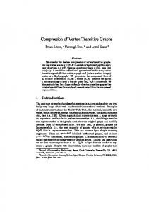
Figure 1: Comparison of α(z) and zc,λ for the 4-regular tree with respect to the automorphism group fixing an end (blue) and the automorphism group fixing a (1, 1, 2)-orientation (red). The second figure is formed by reflecting the first around the line α(z) = 1/2 and then rotating. The intersection of the two curves on the left occurs at (zc , 1). This intersection must occur since zc,0 = zc,1 = zc does not depend on the choice of automorphism group.

4.2

Hammersley-Welsh-type bounds for critically tilted SAW

The Hammersley-Welsh inequality [21] states that, for self-avoiding walk on Zd , we have that h i Z(n) ≤ exp O(n1/2 ) µnc . See [31, Section 3.1] for background and [27] for a small improvement. We now briefly outline how an analogous inequality may be obtained for critically tilted (λ = 1/2) self-avoiding walk in the nonunimodular context. It can be deduced from Corollary 2.7 that h i χ(zt − ε, 1/2) ≤ exp O(ε−1 ) , and applying Lemma 3.4 with cm = Z(1/2; n), x = zt , and y = zt (1 − m−1/2 ) yields that h i Z(1/2; n) ≤ exp O(n1/2 ) µnc,1/2 , which is an exact analogue of the Hammersley-Welsh bound.

4.3

Questions

Question 4.1. Let Tk be a k-regular tree, let d ≥ 1 and consider the group of automorphisms Γξ × Aut(Zd ) ⊆ Aut(Tk × Zd ) of Tk × Zd , where Γξ is the group of automorphisms that fix some specified end ξ of T . 1. Is B(zt ) < ∞? 2. What are the asymptotics of a(zt ; n) and b(zt ; n) as defined in Section 2? 3. What is the behaviour of χ(zt − ε, 1/2) as ε → 0? What about Z(n, 1/2) as n → ∞? 24

4. What is the typical displacement of a SAW sampled from P1/2,n ? 5. For which of these questions does the answer depend on d? Question 4.2. Let G be a connected locally finite graph and let Γ ⊆ Aut(G) be transitive and nonunimodular. Does there exist C = C(G, Γ) < ∞ such that Z(1/2; n) = O nC µnc




for every n ≥ 1? Is there a universal choice of this C? Does C = 1 always suffice? The question concerning C = 1 arises from the guess that the pair (Tk , Γξ ) has the largest subexponential correction to Z(1/2; n) among all pairs (G, Γ). Question 4.3. Let G be a connected locally finite graph and let Γ ⊆ Aut(G) be transitive and nonunimodular. What asymptotics are possible for the typical displacement of a sample from Pn,1/2 ? Is it always of order at least n1/2 ?

Acknowledgments This work was carried out while the author was an intern at Microsoft Research, Redmond. We thank Omer Angel for improving Lemma 3.4 by a factor of 4. We also thank Tyler Helmuth for helpful discussions, and thank Gordon Slade and Hugo Duminil-Copin for comments on an earlier draft.

References [1] R. Bauerschmidt, D. C. Brydges, and G. Slade. Logarithmic correction for the susceptibility of the 4-dimensional weakly self-avoiding walk: a renormalisation group analysis. Comm. Math. Phys., 337(2):817–877, 2015. [2] R. Bauerschmidt, H. Duminil-Copin, J. Goodman, and G. Slade. Lectures on self-avoiding walks. In Probability and statistical physics in two and more dimensions, volume 15 of Clay Math. Proc., pages 395–467. Amer. Math. Soc., Providence, RI, 2012. [3] I. Benjamini. Self avoiding walk on the seven regular triangulation. arXiv preprint arXiv:1612.04169, 2016. [4] I. Benjamini and N. Curien. Ergodic theory on stationary random graphs. Electron. J. Probab., 17:no. 93, 20, 2012. [5] R. Diestel and I. Leader. A conjecture concerning a limit of non-Cayley graphs. J. Algebraic Combin., 14(1):17– 25, 2001. [6] C. Domb and G. Joyce. Cluster expansion for a polymer chain. Journal of Physics C: Solid State Physics, 5(9):956, 1972. [7] H. Duminil-Copin, A. Glazman, A. Hammond, and I. Manolescu. On the probability that self-avoiding walk ends at a given point. Ann. Probab., 44(2):955–983, 2016. [8] H. Duminil-Copin and A. Hammond. Self-avoiding walk is sub-ballistic. Comm. Math. Phys., 324(2):401–423, 2013. p √ [9] H. Duminil-Copin and S. Smirnov. The connective constant of the honeycomb lattice equals 2 + 2. Ann. of Math. (2), 175(3):1653–1665, 2012. [10] L. A. Gilch and S. M¨ uller. Counting self-avoiding walks on free products of graphs. Discrete Mathematics, 340(3):325–332, 2017. [11] G. Grimmett and Z. Li. Self-avoiding walks and the Fisher transformation. Electron. J. Combin., 20(3):Paper 47, 14, 2013.

25

[12] G. R. Grimmett, A. E. Holroyd, and Y. Peres. Extendable self-avoiding walks. Ann. Inst. Henri Poincar´e D, 1(1):61–75, 2014. [13] G. R. Grimmett and Z. Li. Locality of connective constants. 2014. [14] G. R. Grimmett and Z. Li. Strict inequalities for connective constants of transitive graphs. SIAM J. Discrete Math., 28(3):1306–1333, 2014. [15] G. R. Grimmett and Z. Li. Bounds on connective constants of regular graphs. Combinatorica, 35(3):279–294, 2015. [16] G. R. Grimmett and Z. Li. Self-avoiding walks and amenability. 2015. [17] G. R. Grimmett and Z. Li. Cubic graphs and the golden mean. 2016. [18] G. R. Grimmett and Z. Li. Connective constants and height functions for Cayley graphs. Trans. Amer. Math. Soc., 369(8):5961–5980, 2017. [19] G. R. Grimmett and Z. Li. Self-avoiding walks and connective constants, 2017. [20] J. M. Hammersley and K. W. Morton. Poor man’s Monte Carlo. J. Roy. Statist. Soc. Ser. B., 16:23–38; discussion 61–75, 1954. [21] J. M. Hammersley and D. J. A. Welsh. Further results on the rate of convergence to the connective constant of the hypercubical lattice. Quart. J. Math. Oxford Ser. (2), 13:108–110, 1962. [22] T. Hara. Decay of correlations in nearest-neighbor self-avoiding walk, percolation, lattice trees and animals. Ann. Probab., 36(2):530–593, 2008. [23] T. Hara and G. Slade. The lace expansion for self-avoiding walk in five or more dimensions. Rev. Math. Phys., 4(2):235–327, 1992. [24] T. Hara and G. Slade. Self-avoiding walk in five or more dimensions. I. The critical behaviour. Comm. Math. Phys., 147(1):101–136, 1992. [25] T. Hutchcroft. Non-uniqueness and mean-field criticality for percolation on nonunimodular transitive graphs. In preparation. [26] T. Hutchcroft. Critical percolation on any quasi-transitive graph of exponential growth has no infinite clusters. Comptes Rendus Mathematique, 354(9):944 – 947, 2016. [27] T. Hutchcroft. The hammersley-welsh bound for self-avoiding walk revisited. 2017. [28] H. Kesten. On the number of self-avoiding walks. II. J. Mathematical Phys., 5:1128–1137, 1964. [29] Z. Li. Positive speed self-avoiding walks on graphs with more than one end. arXiv preprint arXiv:1612.02464, 2016. [30] R. Lyons and Y. Peres. Probability on Trees and Networks. Cambridge University Press, New York, 2016. Available at http://pages.iu.edu/~ rdlyons/. [31] N. Madras and G. Slade. The self-avoiding walk. Modern Birkh¨ auser Classics. Birkh¨ auser/Springer, New York, 2013. Reprint of the 1993 original. [32] N. Madras and C. C. Wu. Self-avoiding walks on hyperbolic graphs. Combinatorics, Probability and Computing, 14(4):523–548, 2005. [33] A. Nachmias and Y. Peres. Non-amenable Cayley graphs of high girth have pc < pu and mean-field exponents. Electron. Commun. Probab., 17:no. 57, 8, 2012. [34] B. Nienhuis. Exact critical point and critical exponents of O(n) models in two dimensions. Phys. Rev. Lett., 49(15):1062–1065, 1982. [35] I. Pak and T. Smirnova-Nagnibeda. On non-uniqueness of percolation on nonamenable Cayley graphs. C. R. Acad. Sci. Paris S´er. I Math., 330(6):495–500, 2000. [36] P. M. Soardi and W. Woess. Amenability, unimodularity, and the spectral radius of random walks on infinite graphs. Math. Z., 205(3):471–486, 1990. ´ Tim´ [37] A. ar. Percolation on nonunimodular transitive graphs. The Annals of Probability, pages 2344–2364, 2006.

26