Self-consistent random-phase approximation for interacting electrons ...

PHYSICAL REVIEW B 66, 085318 共2002兲

Self-consistent random-phase approximation for interacting electrons in quantum wells and intersubband absorption Sergey V. Faleev1,2 and Mark I. Stockman1,* 1

Department of Physics and Astronomy, Georgia State University, Atlanta, Georgia 30303 2 Sandia National Laboratories, Livermore, California 94551 共Received 23 September 2001; revised manuscript received 1 February 2002; published 20 August 2002兲 For electrons with Coulomb interaction confined in a quantum well, we have developed an approach based on the Kadanoff-Baym-Keldysh technique to calculate equilibrium Green’s functions. This approach is based on iterative numerical computation of the retarded self-energy in the self-consistent random-phase approximation. For two subbands, at zero temperature, we have computed spectral functions, electron distributions, quasiparticle spectra, and the current-current correlation function that determines the intersubband absorption coefficient. Our computations of the optical absorption take into account the depolarization shift and vertex corrections. Apart from direct applications of this theory to the physics of semiconductor quantum well devices, the Green’s functions obtained may also serve as self-consistent initial conditions for quantum kinetics problems in quantum wells. DOI: 10.1103/PhysRevB.66.085318

PACS number共s兲: 73.21.⫺b, 05.30.Fk, 78.67.⫺n

I. INTRODUCTION

Intersubband absorption of electrons in quantum wells is among the most important properties from both fundamental and applied positions. In particular, one of the most developed and frequently used applications of quantum wells is quantum-well infrared photodetectors 共see, e.g., Refs. 1–3兲. For this application, and many others, electron densities are high enough in order to yield sufficiently high responses. Consequently, significant effects of many-body electronelectron interaction are present in the intersubband absorption 共see, e.g., Sec. 2.7.2 in Ref. 1 and Chap. 4 in Ref. 2兲. The intersubband absorption is also of high significance for another important application of quantum wells, namely, quantum cascade lasers.4 In this paper, we develop a theory of intersubband absorption based on the fully self-consistent random-phase approximation 共also known as the GW approximation兲, and apply it to intersubband absorption in specific quantum-well infrared photodetectors. Another perspective application of the present results is the description of an initial correlated electron state for ultrafast physics. Stimulated by the development of ultrashort laser pulses, theoretical and experimental studies of ultrafast kinetics of interacting electrons in semiconductors have experienced rapid development. This problem is very interesting and theoretically complicated due to the fact that manybody Coulomb interaction on a very short time scale is not efficiently screened and therefore is very strong.5–13 From the applied point of view, the research on the ultrafast kinetics promises important contributions to the physics of ultrafast electronic and optoelectronic devices. Significant theoretical progress in this field has recently been obtained on the basis of the nonequilibrium Green’s-function method by Kadanoff and Baym14 and Keldysh.15 This method has been further developed by Langreth16 and Rammer and Smith.17 It is widely recognized that the conventional equilibrium field-theoretical technique 共described, e.g., in Ref. 18兲 is not applicable to the ultrafast kinetic problems where the Kadanoff-Baym-Keldysh 共KBK兲 method of nonequilibrium Green’s-functions is valid and should be used. However, it is 0163-1829/2002/66共8兲/085318共11兲/$20.00

much less appreciated that the equilibrium Green’s-function method may also not be applicable to the interaction of light with many-body systems, because this method is based on an adiabatic switching-on the interactions, while, in contrast, the light field is rapidly oscillating. Therefore, even for the continuous-wave 共cw兲 excitation of many-electron systems, the nonequilibrium KBK approach may be necessary. The KBK method also has an added advantage that the initial 共equilibrium兲 electron system can be conveniently treated at a given finite temperature. It is necessary to mention that there has been a significant amount of work done in the field of interacting electrons using the well-known semiconductor Bloch equations 共SBE’s兲 共see, e.g., Ref. 19兲. In contrast to the two-time KBK equations, the SBE’s are single-time equations that can be obtained from the KBK equations by using additional approximations. In particular, they can be derived from the KBK equations using the generalized Kadanoff-Baym ansatz 共see, e.g., Ref. 20兲 whose accuracy is not quite controllable. This ansatz cannot be derived consistently microscopically and expressed as a result of a summation of some subset of contributions 共diagrams兲. Some additional approximations such as use of the zero-order retarded and advanced Green’s functions also are invoked.20 In the present paper, we consider intersubband optical absorption for the electrons in the conduction band of a quantum well. As the necessary first stage of this project and of separate interest, we find equilibrium many-body Green’s functions of the electrons in the quantum well, taking into account the two lowest subbands. The KBK technique used by us provides a unified and powerful method of solving both these problems, equilibrium and nonequilibrium 共optical兲. As we already mentioned above, the equilibrium Green’s functions of the KBK theory, that we have determined in this research, can also be used as initial conditions in the future studies on ultrafast intersubband kinetics of interacting electrons in quantum wells. Because it is impossible to exactly solve the manyelectron Coulomb-interaction problem, one has to resort to approximations. The random phase approximation 共RPA兲 is

66 085318-1

©2002 The American Physical Society

PHYSICAL REVIEW B 66, 085318 共2002兲

SERGEY V. FALEEV AND MARK I. STOCKMAN

the most widely used and realistic approximation for manybody electron problems. Of principal importance is that for the quantum kinetics problems and, generally, for optical excitation problems, the RPA should necessarily be selfconsistent 共SC兲, otherwise the local conservation laws for the electron density and energy-momentum density are violated.21 The self-consistency of the RPA means that Green’s functions that are employed to calculate the polarization operator in the ‘‘bubble’’ approximation ⌸⫽GG and the self-energy in the GW approximation ⌺⫽GW are the final Green’s functions that satisfy the Dyson equation with self-energy ⌺. Note that the theories such as SCRPA that are compatible with the exact conservation laws are called conserving.21 In this respect we note that some theories do not employ a completely self-consistent approximation and, therefore, are not necessarily conserving. As an example, we mention Ref. 22 by Barth and Holm, which is a GW 0 theory, which means that the self-energy ⌺ is calculated with the final Green’s functions G, but the screened 共renormalized兲 interaction is calculated with the non-self-consistent Green’s functions G 0 . In contrast, a later paper23 by the same authors was the first, to our knowledge, example of the application of a fully self-consistent RPA (GW approximation兲, which is conserving, to a 3D electron gas. Taking into account the above-discussed compelling arguments, we earlier employed the SCRPA in the framework of the KBK approach to find the Green’s function and various observable quantities, such as the momentum distribution, one-electron energy, spectral function, etc., of a twodimensional 共2D兲 electron gas at the zero and finite temperatures.24,25 In the present study, we generalize this approach to describe the state and optical absorption of electrons in the conduction subband of a quantum well. Previously, a significant number of theoretical papers were devoted to a computation of the intersubband absorption 共see, e.g., Refs. 26 –29兲. These theories are based on different versions of the RPA, but none of them, distinct from the present theory, is a SCRPA. In qualitative agreement with previous results,26,27 we found a significant depolarization blueshift of the absorption spectrum maximum. However, quantitatively, the self-consistency of the RPA leads to an increase of the total blueshift compared with the usual 共nonself-consistent兲 RPA. We have also evaluated the vertex corrections in the current-current correlation function using the ladder approximation. These corrections result in a small increase of the magnitude of the absorption peak, with an almost nondistinguishable redshift in the peak position. This paper is organized in the following way. In Sec. II we present general equations and their solutions for Green’s functions and optical absorption. Numerical procedures are described in Sec. III. The results of numerical computations are presented in Sec. IV. Finally, concluding remarks are given in Sec. V.

H⫽

⫹

We consider an electron system with the Coulomb interaction confined in quantum well with two subband states. The positive ions are described by a jellium model. The Hamiltonian of the system is

1 2S

兺

i, j,k,l,q,p,p⬘

†

† V i jkl 共 q兲 a i,p⫹q a j,p⬘ ⫺qa k,p⬘ a l,p , 共1兲

where S is the area of the quantum well, ␮ is the chemical potential; p, p⬘ , and q are 2D momentum vectors in the plane of the well, indexes i, j,k,l⫽1,2 denote the subband 共envelope兲 states whose wave functions are ␾ 1 (z) and ␾ 2 (z), with z as the growth direction 共i.e., the normal to the (0) (0) (0) ⫽ p 2 /2m and E 2,p ⫽ p 2 /2m⫹E 12 are well plane兲; and E 1,p (0) one-particle energies, where E 12 is the bare energy gap and m is the bare effective mass of the electron. The original 共unscreened兲 Coulomb potential is given by the usual expression V i jkl 共 q兲 ⫽

冕

dzdz ⬘ ␾ * i 共 z 兲␾* j 共 z ⬘ 兲v共 q,z⫺z ⬘ 兲 ␾ k 共 z ⬘ 兲 ␾ l 共 z 兲 , 共2兲

where v共 q,z 兲 ⫽

冕

d 2 re iqr

e2

⑀ b 冑r2 ⫹z

⫽ 2

2 ␲ e 2 ⫺q 兩 z 兩 e . ⑀ bq

⑀ b is the background dielectric constant, and e is the electron charge. The subband wave functions in the absence of a magnetic field can be chosen real, so the potential V i jkl of Eq. 共2兲 has the following permutation symmetry: V i jkl ⫽V l jki ⫽V ik jl ⫽V jilk . In the following we assume that the well is symmetric with respect to its middle (z⫽0); therefore the wave functions have a definite parity: ␾ 1 (⫺z)⫽ ␾ 1 (z) and ␾ 2 (⫺z)⫽⫺ ␾ 2 (z). In this case, only four independent matrix elements of V i jkl do not vanish, which we denote V 1 (q) ⬅V 1111(q), V 2 (q)⬅V 2222(q), V c (q)⬅V 1221(q), and V x (q) ⬅V 1212(q). The Kadanoff-Baym 共KB兲 equations are formulated for a set of four Green’s functions: greater G ⬎ , lesser G ⬍ , retarded G r , and advanced G a . Similar notations are used for the components of other field-theoretical objects, such as the self-energy ⌺, polarization operator ⌸, dynamicallyscreened interaction W, etc. We deal with equilibrium uniform systems where the Green’s functions depend only on a conserving momentum p and time difference t, and are defined in the momentum-time representation as † G⬍ i 共 p,t 兲 ⫽i 具 a i,p共 0 兲 a i,p共 t 兲 典 , † G⬎ i 共 p,t 兲 ⫽⫺i 具 a i,p共 t 兲 a i,p共 0 兲 典 ,

II. THEORY AND BASIC EQUATIONS A. Green’s functions

(0) † ⫺ ␮ 兲 a i,p a i,p 共 E i,p 兺 i,p

共3兲

where the angular brackets denote quantum-mechanical averaging and averaging over the Gibbs ensemble; we do not show the spin indices over which all objects are diagonal. Also, the equilibrium Green’s functions are diagonal over subband indexes due to conserved parity in the absence of external electrical field.

085318-2

PHYSICAL REVIEW B 66, 085318 共2002兲

SELF-CONSISTENT RANDOM-PHASE APPROXIMATION . . .

For any object A of the theory 共the Green’s function G, self-energy ⌺, dynamically screened potential W, polarization operator ⌸, etc.兲, the corresponding retarded 共r兲 and advanced 共a兲 components are expressed as ⬎

⬍

A 共 p,t 兲 ⫽⫾ ␪ 共 ⫾t 兲关 A 共 p,t 兲 ⫺A 共 p,t 兲兴 ⫹ ␦ 共 t 兲 A , 共4兲 r,a

where we used the known Langreth rules for the concatenation of two Green’s functions.16 From this, using Eqs. 共5兲 and 共6兲 and the symmetry relation ⬍ ⌸⬎ i j 共 p, ␻ 兲 ⫽⌸ ji 共 p,⫺ ␻ 兲 ,

s

where the second 共singular in time兲 term ␦ (t)As is not related to A⬎,⬍ , and appears due to concatenation of regular objects with time-singular quantities such as potentials that do not include retardation 关see, e.g., the second integral in the right-hand side of Eq. 共23兲兴. From the four types 共components兲 of each quantity, only three are independent due to an identity Ar ⫺Aa ⫽A⬎ ⫺A⬍ .

共5兲

we compute the imaginary part of the retarded polarization operator: Im⌸ ri j 共 p, ␻ 兲 ⫽

共6兲

Also, the well known Kubo-Martin-Schwinger boundary condition is valid,17 ⬍ G⬎ i 共 p, ␻ 兲 ⫽⫺exp共 ␤ ␻ 兲 G i 共 p, ␻ 兲 ,

1 关 ⌸ ⬍ 共 p,⫺ ␻ 兲 ⫺⌸ ⬍ i j 共 p, ␻ 兲兴 . 2i ji

共12兲

Because ⌸ ri j (p, ␻ ) as a function of ␻ is analytical and has no singularities in the upper half plane, and it tends to zero for ␻ →⬁, the conventional Kramers-Kronig relation allows one to restore its real part,

In a stationary case, there is a symmetry relation between the advanced and retarded components of an object in the momentum-frequency representation: Aa * 共 p, ␻ 兲 ⫽Ar 共 p, ␻ 兲 .

共11兲

Re⌸ ri j 共 p, ␻ 兲 ⫽

1 P ␲

冕

d␻⬘

Im⌸ ri j 共 p, ␻ ⬘ 兲

␻ ⬘⫺ ␻

共13兲

,

where P denotes the principal value of the integral. Having found the retarded components of the polarization operator, we write down the system of Dyson equations for the retarded dynamically screened potentials W 1 (p, ␻ ), W 2 (p, ␻ ), W c (p, ␻ ), and W x (p, ␻ ):

共7兲

r r W r1 ⫹V c ⌸ 22 W rc , W r1 ⫽V 1 ⫹V 1 ⌸ 11

where ␤ ⫽1/T and T is temperature in energy units. Using this relation, the number of independent components can be reduced to only one. We choose G r as such an independent component, and the other three are expressed as

r r W r2 ⫹V c ⌸ 11 W rc , W r2 ⫽V 2 ⫹V 2 ⌸ 22 r r W rc ⫹V c ⌸ 22 W r2 , W rc ⫽V c ⫹V 1 ⌸ 11

G ai 共 p, ␻ 兲 ⫽G ri * 共 p, ␻ 兲

r r ⫹⌸ 21 W rx ⫽V x ⫹V x 共 ⌸ 12 兲 W rx .

r G⬍ i 共 p, ␻ 兲 ⫽⫺i2n ␻ Im关 G i 共 p, ␻ 兲兴 ,

These Dyson equations describe the ‘‘dressing’’ of the bare potentials V 1 (p), V 2 (p), V c (p), and V x (p) by the chains of corresponding polarization operators. Here and below, we use the known Langreth rules16 that allow one to find components of the product of two objects A and B;

r G⬎ i 共 p, ␻ 兲 ⫽⫺i2 共 n ␻ ⫺1 兲 Im关 G i 共 p, ␻ 兲兴 ,

共8兲

where n ␻ ⫽ 关 exp(␻/T)⫹1兴⫺1 is the Fermi factor, and we use a system of units where ប⫽1. We use an iterative process to find Green’s function G r numerically. As the result of an iterative step, we obtain the retarded self-energy ⌺ ri (p, ␻ ). The following is a description of the next iterative step. Using the Dyson equation for the retarded Green’s function, we find G ri 共 p, ␻ 兲 ⫽

1

␻ ⫺ ␰ i,p⫺⌺ ri 共 p, ␻ 兲

,

共9兲

共 AB兲 r,a ⫽A r,a Br,a ,

冕

W r1 ⫽

V 1⫹

V 2c ⌸ r2

册 册

1

共 1⫺V 1 ⌸ r1 兲共 1⫺V 2 ⌸ r2 兲 ⫺V 2c ⌸ r1 ⌸ r2 1⫺V 1 ⌸ r1

V 2c ⌸ r1 r 共 1⫺V 1 ⌸ 1 兲共 1⫺V 2 ⌸ r2 兲 ⫺V 2c ⌸ r1 ⌸ r2

W rc ⫽

1 1⫺V 2 ⌸ r2

Vc 共 1⫺V 1 ⌸ r1 兲共 1⫺V 2 ⌸ r2 兲 ⫺V 2c ⌸ r1 ⌸ r2

W rx ⫽

⬎ G⬍ i 共 k, ␻ ⬘ 兲 G j 共 k⫺p, ␻ ⬘ ⫺ ␻ 兲 , 3

共10兲

冋 冋

W r2 ⫽ V 2 ⫹

d ␻ ⬘d 2k 共2␲兲

共 AB兲 ⬎,⬍ ⫽A ⬎,⬍ Ba ⫹Ar B ⬎,⬍ . 共15兲

The solutions of Eqs. 共14兲 are

(0) ⫺ ␮ , and i⫽1,2. From this, using Eqs. 共8兲, where ␰ i,p⫽E i,p ⬎,⬍ we find G . This allows us to obtain the electron polarization operator in the RPA 共bubble兲 approximation ⌸⫽GG, or in the detailed form

⌸⬍ i j 共 p, ␻ 兲 ⫽⫺2i

共14兲

Vx r r 1⫺V x 共 ⌸ 12 ⫹⌸ 21 兲

,

,

,

,

共16兲

where we used notations ⌸ 1 ⬅⌸ 11 and ⌸ 2 ⬅⌸ 22 for brevity.

085318-3

PHYSICAL REVIEW B 66, 085318 共2002兲

SERGEY V. FALEEV AND MARK I. STOCKMAN

Using Eqs. 共7兲 and 共10兲, one can derive a relation for the greater and lesser components of the polarization operators, analogous to the relation for Green’s functions 共7兲: ⬍ ⌸⬎ i j 共 p, ␻ 兲 ⫽exp共 ␤ ␻ 兲 ⌸ i j 共 p, ␻ 兲 .

共17兲

In general, this relation can be proved in the same way as the Kubo-Martin-Schwinger boundary condition.17 Using this and applying the Langreth rules 关Eq. 共15兴 to the lesser and greater components of the renormalized potential W that is built from the multiple products of the polarization operators, one can derive that a similar relation is valid for each of the potentials W 1 , W 2 , W c , and W x : ⬎

⬍

W 共 p, ␻ 兲 ⫽exp共 ␤ ␻ 兲 W 共 p, ␻ 兲 .

共18兲

The last integral in the right-hand side of Eq. 共23兲 is the exchange diagram that is ␻ independent, yielding a correct asymptotic behavior of Re⌺ ri (p, ␻ ) for ␻ →⬁. Concluding this subsection, we have started with ⌺ ri 关see the paragraph preceding, Eq. 共9兲兴 and finished with the nextiteration ⌺ ri 关Eqs. 共22兲 and 共23兲兴. This closes the iterative procedure. All the necessary Green’s function are selfconsistently found within the current iteration 关Eqs. 共8兲 and 共9兲兴. B. Intersubband linear absorption spectrum

The linear absorption coefficient ␣ ( ␻ ) is related by the Kubo formula to the imaginary part of retarded currentcurrent correlation function ␲ r ( ␻ ),32

Combining Eqs. 共5兲 and 共6兲 for the renormalized Coulomb potential and using relation 共18兲, we obtain the expression for the lesser component of the potential, ⬍

W 共 p, ␻ 兲 ⫽

2i e ␤ ␻ ⫺1

Im W 共 p, ␻ 兲 , r

共19兲

where W r is given by Eq. 共16兲. The greater component of the dynamically screened potential W can be obtained from symmetry relations ⬎

⬍

W 共 p, ␻ 兲 ⫽W 共 p,⫺ ␻ 兲 , W 共 p, ␻ 兲 ⫽W 共 p,⫺ ␻ 兲 . a

r

共20兲

To complete the current iteration step, we compute the lesser and greater self-energies in the SCRPA 共the GW approximation兲 as ⌺ ⬎,⬍ 共 p,␻兲 ⫽i i

冕

d ␻ ⬘d 2k 共2␲兲

3

关 W ⬎,⬍ 共 k, ␻ ⬘ 兲 G ⬎,⬍ 共 p⫺k, ␻ ⫺ ␻ ⬘ 兲 i i

⬎,⬍ ⫹W ⬎,⬍ 共 k, ␻ ⬘ 兲 G 3⫺i 共 p⫺k, ␻ ⫺ ␻ ⬘ 兲兴 . x

共21兲

Taking into account Eqs. 共5兲 and 共6兲, we can express the imaginary part of the retarded self-energy as Im⌺ ri 共 p, ␻ 兲 ⫽

1 ⬎ 关 ⌺ 共 p, ␻ 兲 ⫺⌺ ⬍ i 共 p, ␻ 兲兴 . 2i i

共22兲

Finally, Re⌺ ri is found from a dispersion relation 1 Re⌺ ri 共 p, ␻ 兲 ⫽ P ␲ ⫺

冕

冕

d␻⬘

Im⌺ ri 共 p, ␻ ⬘ 兲

2

␲ r共 ␻ 兲 ⫽ 兩 p z兩 2S

Im ␲ r 共 ␻ 兲 ,

共25兲

r ⌸ 21 共 q⫽0,␻ 兲 r 1⫺V x 共 q⫽0 兲 ⌸ 21 共 q⫽0,␻ 兲

,

r ⌸ 21 共 q⫽0,␻ 兲 ⫽⫺2i

共23兲

d␻ ⬍ G 共 ␻ ,p兲 . 2␲ i

共24兲

共26兲

where p z ⫽(e/m) 兰 dz ␾ 2 (z)(d/dz) ␾ 1 (z) is the matrix element of the current between the two subbands, where we assume that the exciting light is linearly polarized in the growth 共z兲 direction of the quantum well. In Eq. 共26兲, we neglect the small ⌸ 12 polarization operator and retain only the ⌸ 21 polarization operator that describes the resonant absorption of the light when an electron undergoes the transition from subband 1 to subband 2, which is the well-known resonant or rotating-wave approximation. In the SCPRA r is 共‘‘bubble’’ approximation兲, the polarization operator ⌸ 21 given by Eqs. 共10兲–共13兲. Note that Eq. 共26兲 is applicable to both single and multiple quantum wells, where in the latter case V is the system’s volume per one quantum well. To go beyond the ‘‘bubble’’ approximation, we need to calculate corrections to the vertex ⌫(p, ␻ ⬘ ). We use the ladder approximation which is the most common approximation for the vertex corrections. To study the vertex corrections to the polarization operator, we present this operator as the concatenation of the intersubband 共nondiagonal over subband indices兲 Green’s function G 21 in the presence of an electromagnetic field with frequency ␻ ,

冕

d ␻ ⬘d 2p 共2␲兲

3

⬍ G 21 共 p, ␻ ⫹ ␻ ⬘ , ␻ ⬘ 兲 ,

共27兲

where this intersubband Green function G 21 is related to the vertex ⌫ as G 21共 p, ␻ ⫹ ␻ ⬘ , ␻ ⬘ 兲 ⫽G 2 共 p, ␻ ⫹ ␻ ⬘ 兲 ⌫ 共 p, ␻ ⫹ ␻ ⬘ , ␻ ⬘ 兲

where the momentum distribution function n i (p) for each subband is expressed as

冕

冑⑀ b V ␻

关 V i 共 k兲 n i 共 pÀk兲

⫹V x 共 k兲 n 3⫺i 共 pÀk兲兴 ,

n i 共 p兲 ⫽⫺i

4␲

where V is the 3D volume of the system. This retarded current-current correlation function is given by

␻ ⬘⫺ ␻

d 2k 共2␲兲

␣ 共 ␻ 兲 ⫽⫺

⫻G 1 共 p, ␻ ⬘ 兲 .

共28兲

We exclude the matrix element of the current from the vertex, so the pure SCRPA corresponds to ⌫⫽1. In Eq. 共27兲, the

085318-4

PHYSICAL REVIEW B 66, 085318 共2002兲

SELF-CONSISTENT RANDOM-PHASE APPROXIMATION . . .

retarded component of the polarization operator is related to the lesser component of the intersubband Green’s function because the Langreth rule16 for the retarded component of two operators concatenated into a loop are exactly the same as for the lesser component of product of these two operators in Eq. 共15兲. We use an iterative process to find the intersubband Green’s function G 21(p, ␻ ⬘ ) numerically for each light frequency ␻ independently. As the result of an iterative step, we obtain three components of the vertex function ⌫ ⬍,r,a (p, ␻ ⬘ ). The following is the description of the next iterative step. Using the Langreth rules of Eqs. 共15兲 and 共28兲, we can determine the components of the G 21 functions r,a r,a r,a ⫽G r,a G 21 2 ⌫ G1 , ⬍ r ⬍ a ⬍ a a G 21 ⫽G r2 ⌫ r G ⬍ 1 ⫹G 2 ⌫ G 1 ⫹G 2 ⌫ G 1 .

共29兲

Note that in contrast to Eq. 共6兲, the retarded and advanced components of the Green’s function G 21 are not related by r a ) * ⫽G 21 兴. complex conjugation 关in fact, (G 12 To complete the iteration cycle, we calculate the vertex function ⌫ in the ladder approximation, where it satisfies the equations ⌫ ⬍ 共 p, ␻ ⫹ ␻ ⬘ , ␻ ⬘ 兲 ⫽i

冕

d ␻ ⬙d 2k 共 2␲ 兲3

⬍ G 21 共 k, ␻ ⫹ ␻ ⬙ , ␻ ⬙ 兲 W ⬍ c 共 p⫺k, ␻ ⬘ ⫺ ␻ ⬙ 兲 ,

⌫ r,a 共 p, ␻ ⫹ ␻ ⬘ , ␻ ⬘ 兲 ⫽1⫹i

冕

d ␻ ⬙d 2k 共 2␲ 兲3

r,a 关 G 21 共 k, ␻ ⫹ ␻ ⬙ , ␻ ⬙ 兲

⬍ ⫻W ⬍ c 共 p⫺k, ␻ ⬙ ⫺ ␻ ⬘ 兲 ⫹G 21共 k, ␻

⫹ ␻ ⬙ , ␻ ⬙ 兲 W r,a c 共 p⫺k, ␻ ⬘ ⫺ ␻ ⬙ 兲兴 , 共30兲 where we used the relations of Eq. 共20兲 for the greater component of the potential W ⬎ . III. NUMERICAL PROCEDURES A. Numerical procedures for Green’s functions in equilibrium

We have numerically solved the equations for the Green’s function in equilibrium using the iterative procedure described above in Sec. II A. Though these equations are valid for arbitrary temperatures, in this paper we have performed computations for T⫽0. Our motivation for this choice is that we intend to concentrate on effects of Coulomb interaction for electrons in a quantum well with two subbands taken into account. A finite temperature will bring about additional effects that will be considered elsewhere. Also, the previous RPA calculations for intersubband absorption spectra,26,27 with which we compare, were carried out at T⫽0. We choose the confining well potential to be zero in the well region, z苸(⫺d/2,d/2), and infinite elsewhere. Thus the ground-state and first-exited-state wave functions are

␾ 1 共 z 兲 ⫽ 冑2/d cos共 ␲ z/d 兲 ,

␾ 2 共 z 兲 ⫽ 冑2/d sin共 2 ␲ z/d 兲 , 共31兲 where the width d of the well is related to the bare intersub(0) (0) as d⫽ 冑3/(2mE 12 ). Using these wave funcband gap E 12 tions, the integrals of Eq. 共2兲 are easily calculated analytically. The final electron density of the system is controlled by the chemical potential ␮ . One can convince oneself that all dimensionless quantities of the theory depend only on two (0) dimensionless parameters r s0 ⬅e 2 冑m 兩 ␮ 兩 /( ⑀ b ␮ ) and E 12 /兩␮兩. Note that for interacting electrons, the chemical potential is not necessarily positive. Alternatively, it is convenient to present the results as functions of two ‘‘dressed’’ dimensionless parameters: a conventional density parameter 共that is the relative distance between electrons兲 r s and a relative bare (0) /␧ F . For a 2D electron gas, r s intersubband gap ␳ ⫽E 12 2 ⬅me / ⑀ b 冑␲ n, where n⫽2 兺 i 兰 n i (p)d 2 p/(2 ␲ ) 2 is the electron density. The Fermi energy ␧ F is conventionally related to the Fermi momentum p F at which the discontinuity in the electron momentum distribution occurs: ␧ F ⬅ p F2 /(2m). In the numerical integrations in Eqs. 共10兲, 共13兲, 共21兲, 共23兲, and 共24兲, the integration over the momentum variables has been truncated at the maximum momentum p max that is 共depending on the r s0 ) from 6 –10 times the Fermi momentum p F . The frequency 共energy兲 integrations were carried out 2 /m. within the region 兩 ␻ 兩 ⬍ p max We ran the iterative procedure described above in Sec. II A until the self-energies ⌺ ri (p, ␻ ) converged 共uniformly in p and ␻ ) within ⭐1% mismatch. This requires about 15 iterations and takes ⬇100 h of CPU time on an SGI Origin 2000 workstation. This iterative procedure has been wellconverging and stable. We found earlier for a 2D electron gas24,25 that such an iterative procedure converged for r s ⭐2.62; the values used in this paper are well within this range. As the initial self-energy we have used either the result24 of a pure 2D case with the same value of r s0 for ⌺ r1 (p, ␻ ) and a small constant value for ⌺ r2 (p, ␻ ), or the result of a previous SCRPA run with a different value of r s0 . There was no appreciable dependence of the final results on the initial value of ⌺ ri (p, ␻ ), implying a good convergence. Integrating over the angle between p and k and over ␻ ⬘ , we divided the integration interval into 20– 40 segments to take advantage of the smooth behavior of the integrands in some segments. The number of segments was chosen to optimize the computational efficiency. The adaptive Romberg integration of fifth-order accuracy was used to integrate over each of these segments. This method allowed us to achieve a relative error of integration of less than 10⫺4 . We computed the self-energies and polarization operators in 200– 400 points in their arguments p and ␻ . We verified that the results obtained are stable and do not depend appreciably on any of the computational parameters mentioned above within their indicated range. B. Numerical procedures for optical absorption including vertex corrections

In the integrals in Eqs. 共30兲, a numerical integration was performed following a numerical procedure similar to that

085318-5

PHYSICAL REVIEW B 66, 085318 共2002兲

SERGEY V. FALEEV AND MARK I. STOCKMAN

FIG. 1. Electron momentum distributions for the first and second subbands, n 1 (p) and n 2 (p), calculated in the SCRPA approximation. Curves 1– 4 correspond to the pairs of parameters: 兵 r s , ␳ 其 ⫽ 兵 0.7,1.35其 , 兵 1.06,3.13其 , 兵 1.69,7.85其 , and 兵 2.17,3.46其 .

described in Sec. III A. We ran the iterations of Eqs. 共29兲 and r,a,⬍ (p, ␻ 共30兲 until the intersubband Green’s functions G 21 ⫹ ␻ ⬘ , ␻ ⬘ ) converged 共uniformly in p and ␻ ) within a ⭐1% mismatch. This convergence is very fast, and it requires only from 2– 4 iterations to achieve the required accuracy. Each iteration takes typically ⬇10 h of CPU time on an SGI Origin 2000 workstation for each point in light frequency ␻ . We have used eight processors in parallel to find G 21 in different points over ␻ . As the initial ⌫ we used either ⌫⫽1 or the result of a previous run with a different value of ␻ . There was no appreciable dependence of the final results on the initial values of ⌫ r,a,⬍ (p, ␻ ⫹ ␻ ⬘ , ␻ ⬘ ), signifying a good convergence. IV. NUMERICAL RESULTS

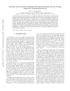
FIG. 2. Quasiparticle dispersion curves for the first and second subbands, E 1 (p) and E 2 (p), are plotted for the four different values of pairs 兵 r s , ␳ 其 indicated in the figure.

among them the SCRPA (GW approximation兲, automatically satisfy this fundamental relation. Note that the conventional 共non-self-consistent兲 RPA (G 0 W 0 approximation兲 is not conserving: it does not conserve the number of particles 共in the presence of a weak probe field兲 and, consequently, does not satisfy this fundamental relation.31 Another quantity of interest is the quasiparticle spectrum in each subband. The quasiparticle energy for a subband is defined as the solution of the equation

A. Equilibrium electron properties

The momentum distributions n i (p) for electrons in each subband (i⫽1,2) are shown in Fig. 1 as a function of p/p 12 for four different pairs of governing parameters r s and ␳ . (0) Here p 12⫽ 冑2mE 12 is the momentum corresponding to the (0) . The values of these govbare intersubband energy gap E 12 erning parameters in our computations are 兵 r s , ␳ 其 ⫽ 兵 0.7,1.35其 , 兵 1.06,3.13其 , 兵 1.69,7.85其 , and 兵 2.17,3.46其 . These values completely define all dimensionless characteristics of the system. Note that the first three cases correspond (0) ⬀ ␳ /r s2 to the same bare intersubband gap, where E 12 ⫽const. We have chosen ␳ ⬎1 in all four cases, which means that the Fermi level lies below the excited subband 共the interaction only increases the final ‘‘dressed’’ intersubband gap, as we will see below in Fig. 2兲. Hence the population of second subband is small at zero temperature, n 2 (p)⬃10⫺3 , as we see in Fig. 1. The dependence n 1 (p) has an expected shape for a normal 共Landau-type兲 Fermi fluid at T⫽0 with a discontinuity at the Fermi momentum p F and a smooth dependence elsewhere. In contrast, the electron momentum distributions in the excited subband are smooth everywhere, as expected. The Fermi momentum p F is completely defined by the position of the discontinuity in n 1 (p) in Fig. 1. On the other hand, it is an exact statement of the Landau Fermi-liquid theory that 共in a 2D case兲 that n⫽p F2 /2␲ . This is a nontrivial fundamental relation and an independent condition that we checked numerically to be valid within the expected accuracy 共margin of error less than 1% for all 兵 r s , ␳ 其 considered兲. This compliance is not accidental: the general theory by Baym30 shows that all so-called conserving approximations,

(0) ⫺ ␮ ⫹Re⌺ ri 关 p,E i 共 p兲兴 . E i 共 p兲 ⫽E i,p

共32兲

The quasiparticle dispersion curves for both subbands are shown in Fig. 2 for the four values of the parameter pairs used in the computations, as indicated in the figure. As one can see, these curves for the first and second subbands are somewhat nonparallel, reducing the transition energy for larger momenta. This effect leads, in particular, to a broadening of the intersubband absorption spectra 共cf. Sec. IV B兲. Another interesting effect is the widening of the intersubband spectral gap E 12⬅E 2 (p⫽0)⫺E 1 (p⫽0) due to the interaction. For the parameters of Figs. 2共a兲–2共d兲, the relative change of E 12 with respect to the Fermi energy is calculated (0) )/␧ F ⫽0.31, 0.59, 1.14, and 1.25. This into be (E 12⫺E 12 crease of the relative shift with r s is an expected consequence of the screening that becomes less efficient at lower electron densities. A less obvious effect is that the absolute shift still decreases with increase of r s 共i.e., with decrease of the electron density兲, as one can easily verify. To discuss these dispersion curves, the ground subband energy 共in the units of the Fermi energy兲 E 1 (p)/␧ F at p⫽0 in Fig. 2 is less than ⫺1 关by convention, E 1 (p F )⫽0兴. This means that the ground-subband quasiparticle energies inside the Fermi sphere are lowered relative to those of noninteracting electrons due to the electron correlations taken into account by the SCRPA. This effect is closely related to the decrease of the total energy of the system when the correlations between the electrons are taken into account. Such a decrease of the total energy when ‘‘good’’ 共correlated兲 electron wave functions are used is expected from the general variational principle. It can also be considered as analogous

085318-6

PHYSICAL REVIEW B 66, 085318 共2002兲

SELF-CONSISTENT RANDOM-PHASE APPROXIMATION . . .

FIG. 3. Scaled spectral functions of the system for the first and second subbands, ␧ F A 1 (p, ␻ ) and ␧ F A 2 (p, ␻ ), found in the SCRPA, are plotted against the relative frequency ␻ /␧ F for 兵 r s , ␳ 其 ⫽ 兵 0.7,1.35其 and the values of momentum p indicated. Note the logarithmic scale.

to the decrease of the total energy and lowering of the oneelectron energies for occupied orbitals when a molecule is formed from atoms. The fact that the SCRPA correctly reproduces this lowering of the one-electron energies inside the Fermi sphere indicates that it better describes the correlated many-electron state. Note that the one-electron energy in the excited subband is increased due to the electron correlations, as may be deduced from the data of Fig. 2. These effects bring about an increase of the intersubband transition energy E 12(p)⫽E 2 (p)⫺E 1 (p), which is one of the causes of the blueshift of the intersubband absorption contour 共see below in Sec. IV B兲. The maximum information on one-electron quantities is contained in the spectral functions of the system:32 A i 共 p, ␻ 兲 ⫽⫺2 Im G ri 共 p, ␻ 兲 .

共33兲

These functions satisfy a sum rule

冕

d␻ A 共 p, ␻ 兲 ⫽1. 2␲ i

共34兲

This sum rule is a nontrivial condition that we have used to check the numerical accuracy of our results. It has been satisfied with an error not exceeding 1%, as expected. Spectral functions A 1 (p, ␻ ) and A 2 (p, ␻ ) are plotted in Fig. 3 against the relative frequency for 兵 r s , ␳ 其 ⫽ 兵 0.7,1.35其 and selected values of momentum p. As we can see, these spectral functions at a given p have sharp peaks at the corresponding quasiparticle energies 共measured from the chemical potential兲 E i (p) defined in Eq. 共32兲. Note that for p ⫽ p F , the spectral function of the first subband A 1 contains a

FIG. 4. Scaled spectral functions plotted against relative frequency ␻ /␧ F for the values of momentum p indicated. Curves 1–3 are plotted for relative spectral function of the first subband ␧ F A 1 (p, ␻ ) for three parameter pairs 兵 r s , ␳ 其 ⫽ 兵 0.7,1.35其 , 兵 1.06,3.13其 , and 兵 1.69,7.85其 , respectively. Curve 4, adopted from Ref. 24 and shown for comparison, corresponds to the scaled spectral function ␧ F A(p, ␻ ) for a pure 2D electron gas with r s ⫽1.16.

␦ -function peak at ␻ ⫽0, while the spectral function for the excited subband does not have a ␦ -function singularity since it actually corresponds to electrons above the Fermi surface. Numerically, the ␦ -function peak has a very small width introduced for the regularization required by the computational procedures through a small negative addition to Im⌺ r for a narrow region around ␻ ⫽0. Interesting scaling properties of the spectral functions can be traced in Fig. 4 where we show the scaled spectral functions for the first subband, ␧ F A 1 (p, ␻ ), for three values of the parameter pairs 兵 r s , ␳ 其 ⫽ 兵 0.7,1.35其 , 兵 1.06,3.13其 , and 兵 1.69,7.85其 共curves 1–3兲. As curve 4, we show a scaled spectral function ␧ F A( p, ␻ ) for a 2D electron gas with r s ⫽1.16 adopted from our previous work,24 which formally corresponds to 兵 r s , ␳ 其 ⫽ 兵 1.16,⬁ 其 . As we see from this figure, in the vicinity of the quasiparticle peak, the scaled quantity ␧ F A 1 is with a good accuracy a universal function of ␻ /␧ F . Though this universal behavior is not yet understood analytically, it is very pronounced: the curves in Fig. 4 corresponding to the same p/p F practically coincide for different 兵 r s , ␳ 其 . The deviation from this universal behavior is seen only for far wings where the spectral function itself is small. Note that a similar universality for the 2D case was discovered in Ref. 24. B. Optical absorption results

We define normalized 共dimensionless兲 absorption function ˜␣ ( ␻ ) by a relation

085318-7

PHYSICAL REVIEW B 66, 085318 共2002兲

SERGEY V. FALEEV AND MARK I. STOCKMAN

TABLE I. Absorption peak position ␻ m , its depolarization shift ⌬ ␻ m , and the bare intersubband gap E (0) 12 in the units of the Fermi energy ␧ F . The data are shown for the four cases of parameters r s and ␳ ⫽E (0) 12 /␧ F , corresponding to curves 1-4 in Fig. 1; the labels RPA and SCRPA indicate the corresponding approximation. For ␻ m in the SCRPA, we include the depolarization shift and vertex corrections, while in the RPA we use Eq. 共36兲.

rs

FIG. 5. The normalized intersubband absorption function ˜␣ ( ␻ ) calculated in the SCRPA approximation plotted as a function of the relative frequency ␻ /␧ F for different values of parameter pairs 兵 r s , ␳ 其 indicated. Curve 1 is for both the depolarization effect and vertex corrections taken into account, curve 2 includes only the depolarization effect, and curve 3 is calculated disregarding both the depolarization effect and vertex corrections 共see the text for details兲.

˜␣ 共 ␻ 兲 ⫽ ␣ 共 ␻ 兲 L 冑⑀ b ,

共35兲

where L⫽V/S is the length 共in the growth direction兲 of the system per a quantum well. This function ˜␣ ( ␻ ) depends only on the two parameters of the system: r s and ␳ . The normalized absorption function ˜␣ ( ␻ ) is shown in Fig. 5 in three different approximations for different values of 兵 r s , ␳ 其 parameters as a function of relative frequency ␻ /␧ F . Curve 1 denotes the complete result with the depolarization shift and vertex corrections as given by Eq. 共25兲 and the subsequent equations in Sec. II B. Curve 2 is computed without the vertex corrections, i.e., setting ⌫(p, ␻ ⫹ ␻ ⬘ , ␻ ⬘ ) ⫽1 in Eq. 共28兲. Furthermore, curve 3 is calculated without the vertex corrections or depolarization effect, which additionally implies setting V x (q)⫽0 in Eq. 共26兲. As one can see from Fig. 5, the depolarization effect, which is described by the denominator on the right-hand side of Eq. 共26兲, dramatically affects the absorption function 共cf. curves 2 and 3兲: in its presence, the absorption contour 共curve 2兲 is approximately four times lower and significantly blueshifted compared with that in the absence of the depolarization effect 共curve 3兲. The absorption contour 共curves 1 and 2兲 is also significantly broadened due to the depolarization effect. This broadening can be traced to the finite width of the spectral function, and physically is due to electrons off the Fermi surface that experience efficient Coulomb scattering. We emphasize that this broadening of the absorption contour is obtained self-consistently within the microscopic theory and is not introduced phenomenologically. Unlike the depolarization effect, the vertex corrections have a small influence on the absorption 共cf. curves 1 and 2兲. Note that in the absence of the depolarization effect 共curve 3兲, the maximum of the absorption peak in frequency closely corresponds to the dressed intersubband separation E 12 . In the usual 共non-self-consistent兲 RPA, where the polarization operator is defined by the bare Green’s functions as

1 2 3 4

RPA

SCRPA

RPA

SCRPA

␧F

␻m ␧F

␻m ␧F

⌬␻m ␧F

⌬␻m ␧F

1.35 3.13 7.85 3.46

1.80 3.61 8.36 4.36

2.15 4.14 9.40 5.45

0.45 0.48 0.50 0.89

0.49 0.43 0.40 0.73

E(0) 12

0.70 1.06 1.69 2.17

⌸⫽G 0 G 0 , the absorption spectrum has the form of a

␦ -function peak. The frequency of the absorption peak in the

RPA was given by Ando and co-workers26,27 as

(0) ␻ mRPA⫽E 12

冉

1⫹

8␲ e 2 n (0) ⑀ b E 12

冕 冋冕 ⬁

⫺⬁

dz

z

⫺⬁

册冊

2 1/2

dz ⬘ ␾ 1 共 z ⬘ 兲 ␾ 2 共 z ⬘ 兲

.

共36兲

The corresponding depolarization shift in the RPA of this RPA RPA (0) ⫽␻m ⫺E 12 . peak is ⌬ ␻ m In Table I we summarize the position of the absorption maxima, ␻ m , in the SCRPA and RPA along with the corresponding shifts of the absorption maxima, ⌬ ␻ m , due to the depolarization effect. For SCRPA this shift is defined as the difference between the coresponding maximum of the abSCRPA sorption spectrum ␻ m and the 共renormalized兲 intersubSCRPA band spectral gap E 12 关see below Eq. 共32兲兴: ␻ m SCRPA ⫽␻m ⫺E 12 . As we can conclude from this table, there is a blueshift of absorption maximum frequency in RPA with respect to the bare intersubband gap, as is known,26 and also a significant further blueshift of the absorption in the SCRPA with respect to the RPA. To pinpoint the origin of this blueshift, we note from Table I that the depolarization shifts in the SCRPA and RPA, though significant, do not differ much. Therefore, the blueshift of the SCRPA with respect to the RPA is mostly due to the widened intersubband gap 共cf. Fig. 2兲 and not due to an increase of the depolarization shift in the SCRPA. It is of considerable interest to compare our theory with experimental data. There exists a significant amount of experimental data for the intersubband optical absorption in quantum wells 共some of such data is reviewed in Ref. 33兲. However, keeping in mind the high application potential of quantum-well infrared photodetectors 共QWIP’s兲, we have chosen to concentrate on the data of Refs. 34 and 35, where QWIP’s were explored. In performing the corresponding calculations, we modified the computational code to take into account the finite heights of the barriers in QWIP’s. Correspondingly, the well energies and wave functions were modified with respect to the infinite-barrier values of Eq. 共31兲.

085318-8

PHYSICAL REVIEW B 66, 085318 共2002兲

SELF-CONSISTENT RANDOM-PHASE APPROXIMATION . . .

FIG. 6. Optical absorbance spectra of electrons for a QWIP with 32 individual quantum wells vs the light wavelength. Solid curve: theory; dashed curve: experiment 共Ref. 34兲. The computations are done for the experimental conditions: 共Ref. 34兲 P polarization at the Brewster angle.

Starting the discussion with the earlier paper,34 the density of the electron gas 共created by a ␦ doping of the quantum wells兲 n⬇9⫻1011 cm⫺2 , corresponding to r s ⬇0.6, is well within our convergence range 共cf. Fig. 1 in Ref. 24兲. The barrier/well composition is Al0.27Ga0.73As/GaAs, the well width is 6 nm, and the barrier width is 25 nm. Note that under these conditions, the first excited one-electron level is at 204 meV, just 15 meV below the barrier top, as deliberately designed for the photodetector functioning. We have calculated the electron absorption spectrum for 30 individual quantum wells in a multiple-quantum-well heterostructure for the above indicated parameters of Ref. 34, except that we have considered the electron-donor dopants as being uniformly distributed inside the quantum well to simplify the computations. The obtained result is displayed in Fig. 6 in comparison with the corresponding experimental absorption spectrum 共see Fig. 2 of Ref. 34兲. Note that both the shape of the absorption contour and the magnitude of the absorption have been calculated and should be compared. We emphasize that our theory does not contain any adjustable parameters. The most important result of our computations is that the calculated absorption spectrum has a significant width, comparable to that of the experimental spectrum. This width is due to the electron-electron interactions that are consistently taken into account in the SCRPA (GW approximation兲, causing the finite lifetimes of the quasiparticles off the Fermi surface, which is also reflected in the width of the spectral function peaks 共cf. Figs. 2 and 3兲. In contrast, the ordinary RPA (G 0 W 0 approximation兲 does not result in any finite spectral widths at zero temperature. Note that the experimental spectrum is still somewhat wider than the theoretical one, which suggests that there are other sources of the broadening, one of them being the nanoroughness of the quantum-well/barrier interface. Another important characteristic, the magnitude of the maximum absorption in Fig. 6, is in an almost perfect agreement with the experiment, but we do not want to overemphasize this fact. The position of the calculated spectral maximum is blueshifted by ⬇12%. The origin of this shift is presently not identified. Different factors may contribute to it. One of them is the already mentioned well-interface roughness. The second factor may be the ␦ doping of the well, which is difficult to take into account computationally. Yet another factor is our two-subband approximation, which is necessary due to the computational complexity. Finally, a factor contributing to this shift may be the approximate na-

FIG. 7. Computed optical absorption spectrum in comparison with the experimental responsivity of the QWIP of Ref. 35. Both the quantities are plotted in arbitrary units and are normalized to the maximum value of 1. Solid curve: theory; dashed curve: experiment 共Ref. 35兲.

ture of the present theory both in the treating of the electronelectron interactions and the neglect of the electron-phonon interactions. The second of the experimental papers with which we compare, 共Ref. 35兲, dealt with a QWIP consisting of 20 periods of GaAs quantum wells of 11.8-nm width, each separated by 40-nm Al0.07Ga0.93As barriers. The quantum wells are doped to the electron density of 4.7⫻1010 cm⫺2 corresponding to r s ⬇2.6. This value is close to the boundary of the region of convergence of our numerical procedure, but still is inside that region 共cf. Fig. 1 in Ref. 24兲. The absorption spectrum was not explicitly measured in Ref. 35, but we know from Ref. 34 that the line shapes of the optical absorption and the QWIP responsivity are quite similar. Based on this, in Fig. 7 we compare our computed absorption spectrum with the responsivity spectrum of Ref. 35. In such an evaluation, we are, indeed, able to compare only the corresponding lineshapes, but not the magnitudes. The comparison of the computed and experimental curves in Fig. 7 shows that in this case the computed width of the absorption contour is significant, though appreciably 共about twice兲 smaller than that of the experimental curve. The shape of the experimental spectrum is significantly different featuring a dip at ⬇27.8 nm that is attributed to the absorption of TO⫹TA phonons.35 It is interesting to note that in this case the theoretical contour is redshifted with respect to the experimental one in contrast to Fig. 6, where there is a blueshift. Same possible reasons of the distinctions between the theory and experiment apply as mentioned in the discussion of Fig. 6 above. V. CONCLUDING REMARKS

We have found equilibrium Green’s functions and related one-electron properties and the intersubband absorption function for a system of electrons with Coulomb interaction bound in a quantum well with two subbands. We have employed the self-consistent random phase approximation 共SCRPA兲 in the framework of the Kadanoff-Baym-Keldysh 共KBK兲 Green’s-function method. This approach, in principle, allows one to describe a system at a given arbitrary temperature, though in this paper it has been natural to limit ourselves to the case of zero temperatures. We have used an iterative method24 of solving the highly nonlinear fieldtheoretical equations, which is stable, convergent, and efficient in a wide enough region of electron densities. For the future studies of laser-induced ultrafast kinetics of

085318-9

PHYSICAL REVIEW B 66, 085318 共2002兲

SERGEY V. FALEEV AND MARK I. STOCKMAN

electrons in quantum wells, the present paper is a useful preliminary investigation where the initial correlated state of the electron system to be considered kinetically is found. Note that previous investigations in quantum kinetics of electrons did not use such a microscopically found initial state. In the intersubband-transition model, noncorrelated electrons were used as the initial state.5,8 –10 Another approach7 used relaxation from a uncorrelated, nonstationary state leading to a stationary correlated state that was then employed as the initial state for quantum kinetics. A drawback of this method of preparing a stationary correlated state is the impossibility to obtain a predetermined temperature, in particular, the zero temperature. We note that there exists a method of imaginary time stepping36 that also allows one to build a correlated self-consistent Green’s functions. This method was implemented for nuclear collisions in Ref. 37 using the generalized Kadanoff-Baym ansatz. This imaginary time-stepping method requires both iterations to achieve selfconsistency and a solution of the temporal equations and is, in principle, equivalent to our approach. There is also another prospective application of the present theory to ultrafast processes. The linear reaction of any system to an electromagnetic field that has arbitrary temporal dynamics, but is weak in the magnitude, is determined through the well-known Kubo theory by the many-body Green’s functions of the equilibrium system. In particular, the computation of the corresponding ultrafast polarization will require only a Fourier transform of the corresponding current-current correlation function. Such a function is found in the present paper in the self-consistent random-phase approximation in Sec. II B. We will pursue this line of investigation elsewhere. There has been an important discussion regarding the longitudinal f-sum rule and its relation to the local conservation laws for Green’s functions.38 – 40 This sum rule is formulated for the renormalized Coulomb line W(p, ␻ ) that is a building block of the theory. It was shown21 that the SCRPA 共called a shielded approximation in Ref. 21兲 is a conserving theory where the local conservation laws 共for current, momentum, etc.兲 are satisfied. However, it is known that W(p, ␻ ) in the SCRPA does not fulfill the f-sum rule. It was argued39 that adding Coulomb lines inside the polarization operator would significantly improve the agreement with the f-sum rule. However, such a modification brings about a violation of the local conservation laws.40 In particular, such a violation would completely preclude the use of the obtained solutions for the description of the initial state for quantum kinetics problems. The cause of this violation is that the theory of Ref. 39 is incompatible with the general method of constructing conserving theories by Baym and Kadanoff.21 In this connection, we note that a numerically solvable approximate theory that would simultaneously satisfy the BaymKadanoff conservation conditions and the f-sum rule has not been developed so far. *To whom correspondence should be addressed. Email address: [email protected]; web site: www.phy-astr.gsu.edu/stockman 1 Semiconductor Quantum Wells and Superlattices for LongWavelength Infrared Photodetectors, edited by M.O. Manasreh

An approach to this general problem was given in Ref. 21兲. In the framework of this approach, the Green’s functions were obtained in a conserving theory 共SCRPA, in particular兲. After that, a modified Coulomb line W(p, ␻ ) was calculated using these Green’s functions by solving the Bethe-Salpeter equation. Such a quantity will exactly satisfy the f-sum rule.21,40 However, it is important to bear in mind that such a modified 共‘‘improved’’兲 Coulomb line cannot be used as a building block for the next generation of self-consistent Green’s functions, because the resulting theory would not fit the framework of Ref. 21 and therefore generally would not be conserving. Without repeating the detailed discussion of the results obtained given in Secs. IV A and IV B, let us briefly mention what we consider to be the main results of the paper. We have generalized the method of Ref. 24 from a 2D electron gas to electrons confined in a quantum well with two subbands 共potentially, many subbands can be included in the future兲. The Green’s functions found bear the maximum information on the one-electron properties of the system 共momentum distribution, electron dispersion and lifetimes, etc.兲. That has allowed us, in particular, to find the intersubband optical absorption whose spectral contour is significantly blueshifted with respect to the conventional 共non-selfconsistent兲 RPA and acquires a finite width due to electronelectron scattering. Most of this blueshift is caused by the significant increase of the intersubband separation due to the electron correlations. An additional significant blueshift is caused by the depolarization effect. In contrast, the effect of vertex corrections in the ladder approximation is small albeit noticeable. A wide area of applications of the results obtained will be the description of the intersubband optical absorption in numerous infrared electro-optical devices, in particular, QWIP’s.34,35 The theory of such devices was previously mainly based on phenomenological or semiphenomenological formulas. We have shown that the present theory explains most of the spectral width of the optical responses in QWIP’s and gives reasonable results for the position 共with en error ⬃12–15 %) and spectral shapes of such responses without any adjustable parameters. Another potential application will be the use of the equilibrium Green’s functions obtained in the present study in the capacity of the initial conditions for the quantum kinetics problems of electrons in quantum wells undergoing intersubband excitation.

ACKNOWLEDGMENTS

This work was supported by the Chemical Sciences, Biosciences and Geosciences Division of the Office of Basic Energy Sciences, Office of Science, U.S. Department of Energy. We appreciate useful discussions with S. G. Matsik and A. G. U. Perera. 共Artech House, Boston, 1993兲. K.K. Choi, The Physics of Quantum Well Infrared Photodetectors 共World Scientific, Singapore, 1997兲. 3 Handbook of Thin Film Devices, handbook edited by M.H. Fran2

085318-10

PHYSICAL REVIEW B 66, 085318 共2002兲

SELF-CONSISTENT RANDOM-PHASE APPROXIMATION . . . combe, Vol. 2: Semiconductor Optical and Electro-Optical Devices, edited by A.G.U. Perera and H.C. Liu 共Academic, San Diego, 2000兲. 4 J. Faist and F. Capasso, in Ref. 3, Chap. 7. 5 H. Haug and A.-P. Jauho, Quantum Kinetics in Transport and Optics of Semiconductors 共Springer, New York, 1996兲. 6 R. Binder, H.S. Ko¨hler, M. Bonitz, and N. Kwong, Phys. Rev. B 55, 5110 共1997兲. 7 N. Hang Kwong and M. Bonitz, Phys. Rev. Lett. 84, 1768 共2000兲. 8 N. Hang Kwong, M. Bonitz, R. Binder, and H.S. Ko¨hler, Phys. Stat. Solidi B 206, 197 共1998兲. 9 L. Ba´nyai, Q.T. Vu, B. Mieck, and H. Haug, Phys. Rev. Lett. 81, 882 共1998兲. 10 Q.T. Vu, L. Ba´nyai, H. Haug, F.X. Camescasse, J.-P. Likforman, and A. Alexandrou, Phys. Rev. B 59, 2760 共1999兲. 11 P. Gartner, L. Banyai, and H. Haug, Phys. Rev. B 60, 14 234 共1999兲. 12 Q.T. Vu, H. Haug, W.A. Hu¨gel, S. Chatterjee, and M. Wegener, Phys. Rev. Lett. 85, 3508 共2000兲. 13 M. Bonitz, in Quantum Kinetic Theory 共Teubner, Stuttgart, 1998兲. 14 L.P. Kadanoff and G. Baym, Quantum Statistical Mechanics, 共Benjamin, New York, 1962兲. 15 L.V. Keldysh, Zh. E´ksp. Teor. Fiz. 47, 1515 共1965兲 关Sov. Phys. JETP 20, 1018 共1965兲兴. 16 D.C. Langreth, in Advanced NATO Study Institute, Series B: Physics, edited by J. T. Devreese and V. E. Van Doren 共Plenum, New York, 1967兲, p. 3. 17 J. Rammer and H. Smith, Rev. Mod. Phys. 58, 323 共1986兲. 18 A.A. Abrikosov, L.P. Gor’kov, and I.E. Dzyaloshinskii, Quantum Field Theoretical Methods in Statistical Physics, 2nd ed. 共Pergamon, New York, 1965兲, Chap. 7.

M. Lindberg and S. Koch, Phys. Rev. B 38, 3342 共1988兲. G. Manzke and K. Henneberger, in Progress in Nonequilibrium Green’s Functions, Edited by M. Bonitz, 共World Scientific, Singapore, 2000兲, p. 238. 21 G. Baym and L.P. Kadanoff, Phys. Rev. 124, 287 共1961兲. 22 U. von Barth and B. Holm, Phys. Rev. B 54, 8411 共1996兲; 55, 10 120共E兲 共1997兲. 23 B. Holm and U. von Barth, Phys. Rev. B 57, 2108 共1998兲. 24 S.V. Faleev and M.I. Stockman, Phys. Rev. B 62, 16 707 共2000兲. 25 S.V. Faleev and M.I. Stockman, Phys. Rev. B 63, 193302 共2001兲. 26 T. Ando, Z. Phys. B: Condens. Matter 26, 263 共1977兲. 27 T. Ando, A.B. Fowler, and F. Stern, Rev. Mod. Phys. 54, 437 共1982兲. 28 D. Huang, G. Gumbs, and M.O. Manasreh, Phys. Rev. B 52, 14 126 共1995兲. 29 P. von Allmen, Phys. Rev. B 46, 13 351 共1992兲. 30 G. Baym, Phys. Rev. 127, 1391 共1962兲. 31 P. Garcia-Gonzales and R.W. Godby, Phys. Rev. B 63, 075112 共2001兲. 32 G.D. Mahan, Many-Particle Physics 共Plenum, New York, 1990兲. 33 T. Elsaesser, and M. Woerner, Phys. Rep. 321, 253 共1999兲. 34 A.G. Steele, H.C. Liu, M. Buchanan, and Z.R. Wasilewski, J. Appl. Phys. 72, 1062 共1992兲. 35 A.G.U. Perera, W.Z. Shen, S.G. Matsik, H.C. Liu, M. Buchanan, and W.J. Schaff, Appl. Phys. Lett. 72, 1596 共1998兲. 36 P. Danielewicz, Ann. Phys. 共N.Y.兲 152, 239 共1984兲. 37 H.S. Ko¨hler, Phys. Rev. C 51, 3232 共1995兲. 38 W.-D. Scho¨ne and A. Eguiluz, Phys. Rev. Lett. 81, 1662 共1998兲. 39 D. Tamme, R. Sheppe, and K. Henneberger, Phys. Rev. Lett. 83, 241 共1999兲. 40 A. Eguiluz, Phys. Rev. Lett. 83, 242 共1999兲. 19 20

085318-11