Sep 18, 2010 ... Today's model, of self-improving algorithms, is the closest to traditional .... of
challenges in making this idea work for a self-improving algorithm.
CS369N: Beyond Worst-Case Analysis Lecture #5: Self-Improving Algorithms∗ Tim Roughgarden† September 18, 2010
1
Preliminaries
Last lecture concluded with a discussion of semi-random graph models, an interpolation between worst-case analysis and average-case analysis designed to identify robust algorithms in the face of strong impossibility results for worst-case guarantees. This lecture and the next two give three more analysis frameworks that blend aspects of worst- and average-case analysis. Today’s model, of self-improving algorithms, is the closest to traditional averagecase analysis. The model and results are by Ailon, Chazelle, Comandar, and Liu [1]. The Setup. For a given computational problem, we posit a distribution over instances. The difference between today’s model and traditional average-case analysis is that the distribution is unknown. The goal is to design an algorithm that, given an online sequence of instances — each an independent and identically distributed (i.i.d.) sample — quickly converges to an algorithm that is optimal for the underlying distribution. Thus the algorithm is “automatically self-tuning.” The challenge is to accomplish this goal with fewer “training samples” and smaller space than a brute-force “learn the data model” approach. Main Example: Sorting. The obvious first problem to apply the self-improving paradigm to is sorting in the comparison model, and that’s what we do here. Each instance is an array of n elements, with the ith element drawn from a real-valued distribution Di . A key assumption is that the Di ’s are independent distributions; Section 5.3 discusses this assumption. The distributions need not be identical. Identical distributions are uninteresting in our context, since in this case the relative order of the elements is a uniformly random permutation. Every correct sorting algorithm requires Ω(n log n) expected comparisons in this case, and a matching upper is bound is achieved by MergeSort (say). ∗
c
2009–2010, Tim Roughgarden. Department of Computer Science, Stanford University, 462 Gates Building, 353 Serra Mall, Stanford, CA 94305. Email:
[email protected]. †
1
2
The Entropy Lower Bound
Since a self-improving algorithm is supposed to run eventually as fast as an optimal one for the underlying distribution, we need to understand some things about optimal sorting algorithms. In turn, this requires a lower bound on the running time of every sorting algorithm with respect to a fixed distribution. The distributions D1 , . . . , Dn over x1 , . . . , xn induce a distribution Π over permutations of {1, 2, . . . , n} via the ranks of the xi ’s. (Assume throughout this lecture there are no ties.) As noted earlier, if Π is (close to) the uniform distribution over the set Sn of all permutations, then the worst-case comparison-based sorting bound of Ω(n log n) also applies here in the average case. On the other hand, sufficiently trivial distributions Π can obviously be sorted faster. For example, if the support of Π involves only a constant number of permutations, these can be distinguished in O(1) comparisons and then the appropriate permutation can be applied to the input in linear time. More generally, the goal is to beat the Ω(n log n) sorting bound when the distribution Π has “low entropy”; and there is, of course, an implicit hope that “real data” can sometimes be well approximated by a low-entropy distribution.1 Mathematically, by entropy we mean the following. Definition 2.1 (Entropy of a Distribution) Let D = {px }x∈X be a distribution over the finite set X. The entropy H(D) of D is X
px log2
x∈X
where we interpret 0 log2
1 0
1 , px
(1)
as 0.
For example, H(D) = log2 |X| if D is uniform. When X is the set Sn of all permutations of {1, 2, . . . , n}, this is Θ(n log n). If D puts positive probability on at most 2h different elements, then H(D) ≤ h. [Exercise: prove this assertion. Use convexity to argue that, for a fixed support, the uniform distribution maximizes the entropy.] Happily, we won’t have to work with the formula (1) directly. Instead, we use Shannon’s characterization of entropy in terms of average coding length. Theorem 2.2 (Shannon’s Theorem) For every distribution D over the set X, the entropy H(D) characterizes (up to an additive +1 term) the minimum possible expected encoding length of X, where a code is a function from X to {0, 1}∗ and the expectation is with respect to D. Proving this theorem would take us too far afield, but it is accessible and you should look it up. 1
For sorting, random data is the worst case and hence we propose a parameter to upper bound the amount of randomness in the data. This is an interesting contrast to the next two lectures, where random data is an unrealistically easy case and the analysis framework imposes a lower bound on the amount of randomness in the input.
2
>
0. Conceptually, the big gains from using an optimal search tree instead of standard binary search occur at leaves that are at very shallow levels (and presumably are visited quite frequently).
5.2
Unknown Distributions
The elephant in the room is that the Interlude and Phase II of our self-improving sorter currently assume that the distributions D are known a priori, while the whole point of the self-improving paradigm is to design algorithms that work well for unknown distributions. The fix is the obvious one: we build (near-optimal) search trees using empirical distributions, based on how frequently the ith element lands in the various buckets. More precisely, the general self-improving sorter is defined as follows. Phase I is defined as before and uses O(log n) training phases to identify the bucket boundaries V . The new Interlude uses further training phases to estimate the Bi ’s (the distributions of the xi ’s over the buckets). The analysis in Section 5.1 suggests that, for each i, only the ≈ nǫ most frequent bucket locations for xi are actually needed to match the entropy lower bound. For V and i fixed, call a bucket frequent if the probability that xi lands in it is at least 1/nǫ , and infrequent otherwise. An extra Θ(nǫ log n) training phases suffice to get accurate estimates of the probabilities of frequent buckets (for all i) — after this point one expects Ω(log n) appearances of xi in every frequent bucket for i, and using Chernoff bounds as in Section 4 implies that all of the empirical frequency counts are close to their expectations (with high probability). The algorithm then builds a search tree Tˆi for i using only the buckets (if any) in which Ω(log n) samples of xi landed. This involves O(nǫ ) buckets and can be done in O(n2ǫ ) time and O(nǫ ) space. For ǫ ≤ 12 , this does not affect the O(n log n) worst-case running time bound for every 9
Figure 5: A Delaunay triangulation in the plane with circumcircles shown.
training phase. One can show that the Tˆi ’s are essentially as good as the truncated optimal search trees of Section 5.1, with buckets outside the trees being located via standard binary search, so that the first stepP of Phase II of the self-improving sorter continues to have an expected running time of O( i H(Bi )) = O(n + H(Π(D))). The arguments have a similar flavor to the proof of Lemma 3.1, although the details are a bit different and are left to the reader (or see [1]). Finally, the second and third steps of Phase II of the self-improving sorter obviously continue to run in time O(n) [expected] and O(n) [worst-case], respectively.
5.3
Beyond Independent Distributions
The assumption that the Di ’s are independent distributions is strong. Some assumption is needed, however, as a self-improving sorter for arbitrary distributions Π over permutations provably requires exponential space — intuitively, there are too many fundamentally distinct distributions that need to be distinguished (see [1] for the counting argument that proves this). An interesting open question is to find an assumption weaker than (or incomparable to) independence that is strong enough to allow interesting positive results. The reader is encouraged to go back over the analysis above and identify all of the (many) places where we used the independence of the Di ’s.
10
5.4
Delaunay Triangulations
Clarkson and Seshadhri [2] give a non-trivial extension of the algorithm and analysis in [1], to the problem of computing the Delaunay triangulation of a point set. The input is n points in the plane, where each point xi is an independent draw from a distribution Di . One definition of a Delaunay triangulation is that, for every face of the triangulation, the circle that goes through the three corners of the face encloses no other points of the input (see Figure 5 for an example and the textbook [3, Chapter 9] for much more on the problem). The main result in [2] is again an optimal self-improving algorithm, with steady-state expected running time O(n + H(∆(D))), where H(∆(D)) is the suitable definition of entropy for the induced distribution ∆(D) over triangulations. The algorithm is again an analog of BucketSort, but a number of the details are challenging. For example, while the third step of Phase II of the self-improving sorter — concatenating the sorted results from different buckets — is trivially linear-time, it is much less obvious how to combine Delaunay triangulations of constant-size “buckets” into one for the entire point set. It can be done, however; see [2].
References [1] N. Ailon, B. Chazelle, S. Comandur, and D. Liu. Self-improving algorithms. In Proceedings of the 17th Annual ACM-SIAM Symposium on Discrete Algorithms (SODA), pages 261–270, 2006. [2] K. L. Clarkson and C. Seshadhri. Self-improving algorithms for Delaunay triangulations. In Proceedings of the 24th Annual ACM Symposium on Computational Geometry (SCG), pages 148–155, 2008. [3] M. de Berg, M. van Kreveld, M. Overmars, and O. Schwarzkopf. Computational Geometry: Algorithms and Applications. Springer, 2000. Second Edition.
11