arXiv:physics/0512270v1 [physics.soc-ph] 30 Dec 2005
EPJ manuscript No. (will be inserted by the editor)
Self-learning Mutual Selection Model for Weighted Networks Jian-Guo Liu1 ,a Yan-Zhong Dang1 , Wen-Xu Wang2 , Zhong-Tuo Wang1 , Tao Zhou2 , Bing-Hong Wang2 , Qiang Guo3 , Zhao-Guo Xuan1 , Shao-Hua Jiang1 and Ming-Wei Zhao1 1 2 3
Institute of System Engineering, Dalian University of Technology, Dalian Liaoning, 116023, P R China Department of Modern Physics, University of Science and Technology of China, Hefei Anhui, 230026, P R China School of Science, Dalian Nationalities University, Dalian Liaoning, 116600, P R China Received: date / Revised version: date Abstract. In this paper, we propose a self-learning mutual selection model to characterize weighted evolving networks. By introducing the self-learning probability p and the general mutual selection mechanism, which is controlled by the parameter m, the model can reproduce scale-free distributions of degree, weight and strength, as found in many real systems. The simulation results are consistent with the theoretical predictions approximately. Interestingly, we obtain the nontrivial clustering coefficient C and tunable degree assortativity r, depending on the parameters m and p. The model can unify the characterization of both assortative and disassortative weighted networks. Also, we find that self-learning may contribute to the assortative mixing of social networks. PACS. 05.65.+b Self-organized systems, 87.23.Ge Dynamics of social systems, 87.23.Kg Dynamics of evolution
1 Introduction In recent years, many empirical findings have triggered the devotion of research communities to understand and characterize the evolution mechanisms of complex networks including the Internet, the World-Wide Web, the scientific collaboration networks and so on[1,2,3,4,5,6]. Many empirical evidences indicate that the networks in various fields have some common characteristics. They have a small average distance like random graphs, a large clustering coefficient and power-law degree distribution [1, 2], which is called the small-world and scale-free characteristics. Recent works on the complex networks have been driven by the empirical properties of real-world networks and the studies on network dynamics [7,8,9,10]. The first successful attempt to generate networks with large clustering coefficient and small average distance is that of Watts and Strogatz (WS model) [1]. Another significant model proposed by Barab´ asi and Albert is called scale-free network (BA network) [2]. The BA model suggests that growth and preferential attachment are two main self-organization mechanisms of the scale-free networks structure. However, the real systems are far from boolean structure. The purely topological characterization will miss important attributes often encountered in real systems. Most recently, the access to more complete empirical data allows scientists to study the weight evolution of many real systems. This calls for the use of weighted Send offprint requests to: a Present address:
[email protected]
network representation. The weighted network is often denoted by a weighted adjacency matrix with element wij representing the weight on the edge connecting node i and j. As a note, this paper will only consider undirected graphs where weights are symmetric, i.e. wijP = wji . The strength si of node i is usually defined as si = j∈Γ (i) wij , where the sum runs over the neighbor node set Γ (i). But in some cases, the sum can not reflect the node strength completely. Take the scientific collaboration networks for example, the strength of a scientist include the publications collaborated with others and the publications written only by himself or herself. Inspired by this idea, the P node strength is defined as si = j∈Γ (i) wij + ηi , where ηi is node i’s self-attractiveness. As confirmed by the empirical data, complex networks exhibit power-law distributions of degree P (k) ∼ k −γ with 2 ≤ γ ≤ 3 [11,12] and weight P (w) ∼ w−θ [13], as well as strength P (s) ∼ s−α [12]. The strength usually reveals scale-free property with the degree s ∼ k β , where β > 1 [12,14,15]. Driven by new empirical findings, Barrat et al. have presented a simple model (BBV for short) to study the dynamical evolution of weighted networks [16]. But its disassortative property can not answer the open question: why social networks are different from other disassortative ones? Previous models can generate either assortative networks [17,18,19] or disassortative ones [12,17,18,20,21]. Our work may shed some new light to answer the question: is there a generic explanation for the difference of assortative and disassortative networks.
Please give a shorter version with: \authorrunning and \titlerunning prior to \maketitle
Our model is defined as following. The model starts from N0 = m isolated nodes, each with an initial attractiveness s0 . In this paper, s0 is set to be 1. (i) At each time step, a new node with strength s0 and degree zero is added in the network; (ii) Every node strength of the network would increase by 1 with the probability p; According to the probability (1 − p), each existing node i selects m other existing nodes for potential interaction according to the probability Equ. (1). Here, the parameter m is the number of candidate nodes for creating or strengthening connections, p is the probability that a node would enhance ηi by 1. sj . (1) Πi→j = P k sk − sj P where si = j∈Γ (i) wij + ηi . If a pair of unlinked nodes is mutually selected, then an new connection will be built between them. If two connected nodes select each other, then their existing connection will be strengthened, i.e., their edge weight will be increased by 1. We will see that m and p control the evolution of our network. The evolution of real-world network can be easily explained by our model mechanisms. Take the scientific collaboration networks as an example: the collaboration of scientists requires their mutual status and acknowledgements. A scientists would like to collaborate with others, whom have strong scientific potentials and long collaborating history. On the contrary, he may write paper or publications only by himself. When he publishes paper
(b)
m=1
m=1
0
m=2
10
m=2
m=3
m=3
m=4
0.1
CP(k)
CP(s)
m=5 m=6
30
m=7
25 20 15
m=4 m=5
-1
10
m=6 m=7
10 5 0
0.01
1
2
3
4
5
6
7
-2
10
m 0
1
10
2
10
0
3
10
1
10
10
2
10
3
10
10
k
s 5.5
(d)
5.0
0
10
4
4.5
10
4.0 3.5 3.0 2.5
-1
10
1
2
3
4
5
m=1
3
10
m=3
m=2
si
m
m=3
m=4
-2
10
m=4
m=5
m=5
2
m=6
10
m=6 m=7
m=7
-3
10
0
10
1
10
2
3
10
1
10
2
10
4
10
3
10
10
k
w
i
Fig. 1. (Color online) Numerical results by choosing p = 0.004. The data are averaged over ten independent runs of network size N = 7000. (a)Cumulative probability strength distribution CP (s) with various m. The results are consistent with a power-law distribution CP (s) ∼ sα . The inset reports the obtained values by data fitting (full circles) in comparison with the theoretical prediction α = 2 + z/[(1 − p)2 m2 ] (line). (b) Cumulative probability degree distribution CP (k) with various m, which demonstrates that the degree distributions have power-law tail. (c) Cumulative probability weight distributions with various m, which are consistent with the power-law tail P (w) ∼ wθ . (d) To different m, the average strength si of nodes with connectivity ki . We observe the nontrivial strength-degree correlation s ∼ kβ in the log-log scale.
m=1
103
m=2 m=3
m=3
3
10
m=4
102
m=1
104
m=2
m=4 m=5
m=5 m=6 m=7
s
2 Construction of the model
(a) 1
P (w )
Previous network models often adopt the mechanism that only newly added nodes could select the pre-existing nodes according to the preferential mechanism. However, the evolution picture ignores the fact that old nodes will choose the young nodes at the same time. Inspired by this idea, Wang et al. have presented the mutual selection mechanism, which leads to the creation and reinforcement of connections [20]. But the model ignored the fact that every node would enhance its strength not only by creating new links to others, but also could by self-learning. In this paper, self-learning means that a node enhances its strength only by itself without creating new links to others. Inspired by this idea, we propose a weighted network model that considers the topological evolution under the general mechanisms of mutual selection and self-learning. It can mimic the evolution of many real-world networks. Our microscopic mechanisms can well explain the characteristics of scale-free weighted networks, such as the distributions of degree, weight and strength, as well as the nonlinear strength-degree correlation, nontrivial clustering coefficient, assortativity coefficient and hierarchical structure that have been empirically observed [11,12,22, 23,24,25]. Also, the model appears as a more general one that unifies the characterization of both assortative and disassortative weighted networks.
k
2
m=6
102
m=7
1
10
101 100
100 (a) 0
10
1
10
2
10
3
10
Rank of vertex
4
10
(b) 100
101
102
103
104
Rank of vertex
Fig. 2. (Color online) Zipf plot of the degree and node strength when p = 0.004.
as the sole author, his strength also increases, which can be reflected by η. For technological networks with traffic taking place on them, both the limit of resources and the internal demand of traffic increment for keeping the normal function of the networks may cause the mutual selections.
Please give a shorter version with: \authorrunning and \titlerunning prior to \maketitle
0.3
m=5
m=6
m=6
m=7
m=7
0.2
knn
(
0.0
0.2 5
-0.1 -0.2
0.2 0
)
Ck
0.1
0.3 0
0.1 5 2
-0.3 -0.4 -0.5
0.1 0
10
0.0 5
1
2
10
3
10
k
10
4
0.0 04
3
0.0 03
2 1
k
0.0 02
0.0 01
p
p
m
4
10
0.003
m
0.002
(a)
Fig. 3. (Color online) The scale of C(k) and knn with k for various m when p = 0.004. The data are averaged over 10 independent runs of network size N = 7000.
0.001
1
0
10
3
3
10
2
2
10
5
1
10
4
5
(b)
(a) 0
0.005 0.004
7
6
6
7
10
0.007 0.006
0.0 0 0.0 07 0.0 06 0.0 05
-2
10
r
-1
10
m=4
3
10
m=5
C
m=4
3
(b)
Fig. 5. (Color online) The scale of C and r with various m and p. The data are averaged over 10 independent runs of network size N = 7000.
Hence, the strength si (t) is updated by this rate (a)
p=0.001
0
10
(b)
0
p=0.002
p=0.003
p=0.003
p=0.006
-1
10
p=0.007
p=0.004
-1
CP(k)
CP(s)
p=0.004 p=0.005
10
p=0.005 p=0.006 p=0.007
-2
10
-2
10
-3
10 0
1
10
2
10
10
X dwij (1 − p)2 m2 si dsi P = +p≈ + p. dt dt k sk j
p=0.001
10
p=0.002
0
3
1
10
10
2
10
3
10
10
k
s (c)
Notice that Z X si = i
0
t
P
dsi dt = dt i
(d)
3
10
(3)
Z tXh i (1 − p)2 m2 si P + p dt. 0 k sk i
Thus, Equ. (3) can be expressed by
-1
10
p=0.001
knn
C (k )
p=0.001 p=0.002 p=0.003
-2
10
dsi (1 − p)2 m2 si + p. = dt (1 − p)2 m2 t + pt2
p=0.002
2
10
p=0.003
p=0.004
p=0.004
p=0.005
p=0.005
p=0.006
p=0.006
p=0.007
p=0.007
(4)
1
10 1
10
2
10
3
10
0
10
1
2
10
10
3
When p ∼ O(N −1 ), the solution of Equ. (4) can be obtained approximately as follows
10
k
k
Fig. 4. (Color online) Numerical results by choosing m = 5 with various p. The data are averaged over ten independent runs of network size N = 7000. (a)Cumulative probability strength distributions CP (s) with various p. The results are consistent with a power-law distribution CP (s) ∼ sα . (b) Cumulative probability degree distributions CP (k) with various p, which demonstrate that the degree distributions have powerlaw tail. (c) The clustering coefficient C(k) depending on connectivity k for various p. (d) Average connectivity knn of the nearest neighbors of a node depending on its connectivity k for different p.
Considering the rule that wij is updated only if node i and j select each other, and using the continuous approximation, then the time evolution of weight can be computed analytically as (1 − p)msj (1 − p)msi dwij = P · P dt k(6=i) sk k(6=i) sk (1 − p)2 m2 (si sj ) P . ( k sk )2
where λ=
(5)
(1 − p)2 m2 , (1 − p)2 m2 + z
and z = pN is a constant. Then, we can get that the strength distribution obeys the power-law P (s) ∼ s−α [16] with exponent α=1+
z 1 . =2+ λ (1 − p)2 m2
(6)
One can also obtain the evolution behavior of the weight distribution P (w) ∼ wθ [28], where
3 characteristics of the model
≈
si (t) ∼ tλ ,
θ =2+
2z , (1 − p)2 m2 − z
and the degree distribution P (k) ∼ k −γ , where γ =2+
(2)
(7)
z . (1 − p)2 m2
(8)
By choosing different values of p and m, we perform numerical simulations of networks which is consistent with
4
Please give a shorter version with: \authorrunning and \titlerunning prior to \maketitle
the theoretical predictions. Fig. 1(a)-(d) present the probability distributions of strength, degree and weight, as well as the strength-degree correlation, fixed p = 0.004 and tuned by m. Fig. 1(a) gives the node strength distribution P (s) ∼ sα , which is in good agreement with the theoretical expression Equ. (6). Fig. 1(b) gives the node degree distribution P (k) ∼ k −γ . Fig. 1(c) reports the probability weight distribution, which also shows the power-law behavior P (w) ∼ wθ . Fig. 1(d) reports the average strength of nodes with degree ki , which displays a nontrivial powerlaw behavior s ∼ k β as confirmed by empirical measurements [12]. Fig. 2(a)-(b) show the Zipf plot of the simulation results by fixing a moderate value p = 0.004 and varying m. Fig. 2(a) confirms with the math collaboration network and the Zipf plot of Fig. 1(a) in Ref. [24]. Fig. 3(a)-(b) give the clustering coefficient C(k) depending on connectivity k and the average connectivity knn of the nearest neighbors of a node for various m. From the numerical results, we can obtain the conclusion that the larger the probability p, the larger the effect of exponential correction at the head. However, the power-law tail which again recovers the theoretical exponent expressions can still be observed. Fig. 4 gives the numerical results for various p when m = 5. Depending on the parameters p and m, the unweighted clustering coefficient C, which describes the statistic density of connected triples, and degree assortativity r [26, 27] are demonstrated in Fig. 5. The assortative coefficient r can be calculated from P P M −1 i ji ki − [M −1 i 21 (ji + ki )]2 P 1 , (9) r = −1 P 1 2 2 −1 2 M i 2 (ji + ki ) − [M i 2 (ji + ki )]
where ji , ki are the degrees of the vertices at the ends of the ith edge, with i = 1, 2, · · · , M . From Fig. 5(a), we can find that C for fixed m increases with p slightly, and C for fixed p monotonously increases with m. The clustering coefficient of our model is tunable in a broad range by varying both m and p, which makes it more powerful in modelling real-world networks. As presented in Fig. 5(b), degree assortativity r for fixed p decreased with m, unlike the clustering case. While r for fixed m increases with p slightly. The model can generates disassortative networks for small m and large p, which can best mimic technological networks. At large p and small m, assortative networks emerge and can be used to mimic social networks, such as the scientific collaboration networks. In the model, enhancing the probability p can be considered as the probability that a node would like to study by itself to enhance its attractiveness or prestige. In the competitive social networks, all nodes face many competitors. In order to subsist or gain honorableness, they must enhance their attractiveness or ability by studying themselves or collaborating with others. This explains the origin of assortative mixing in our model and may shed light on the open question: why social networks are different from other disassortative ones? For example, in the scientific collaboration networks, the attractiveness of a scientist could not be represented simple by the publications collaborated with others. Indeed, there are many other important qualities
that will contribute to the attractiveness of a scientist, for instance, the publications written by himself, etc. Perhaps the different self-learning probability contributes to human beings fundamental differences. On the other hand, m indicates the interaction frequency among the network internal components. If m increases, the hubs would link more and more “young” sites. Thus, the reason why the disassortativity of the model is more sensitive to m lies in that collaboration is more important than self-learning in the technological networks. In addition, the components of technological networks are usually physical devices, which can not study by itself. Combining these two parameters together, two competitive ingredients, which may be responsible for the mixing difference in real complex networks, are integrated in our model.
4 Conclusion and Discussion In summary, integrating the mutual selection mechanism between nodes and the self-learning mechanism, our network model provides a wide variety of scale-free behaviors, tunable clustering coefficient, and nontrivial degreedegree and strength-degree correlations, just depending on the probability of self-learning p and the parameter m which governs the total weight growth. All the statistic properties of our model are found to be supported by various empirical data. Interestingly and specially, studying the degree-dependent average clustering coefficient C(k) and the degree-dependent average nearestneighbors degree knn (k) also provides us with a better description of the hierarchies and organizational architecture of weighted networks. Our model may be beneficial for future understanding or characterizing real networks. Due to the apparent simplicity of our model and the variety of tunable results, we believe our present model, for all practical purposes, might be applied in future weighted network research. This work has been supported by the Chinese Natural Science Foundation of China under Grant Nos. 70431001, 70271046 and 70471033.
References 1. D. J. Watts and S. H. Strogatz, Nature 393, 440 (1998). 2. A. -L. Barab´ asi and R. Albert, Science 286, 509 (1999). 3. R. Albert and A. -L. Barab´ asi, Rev. Mod. Phys. 74, 47 (2002). 4. S. N. Dorogovtsev and J. F. F. Mendes, Adv. Phys. 51, 1079 (2002). 5. M. E. J. Newmann, SIAM Rev. 45 167 (2003). 6. X. F. Wang, Int. J. Bifurcat. Chaos 12, 885 (2002). 7. C. -P. Zhu, S. -J. Xiong, Y. -J. Tian, N. Li and K. -S. Jiang, Phys. Rev. Lett. 92 218702 (2004). 8. T. Zhou, B. -H. Wang, P. -L. Zhou, C. -X. Yang and J. Liu, Phys. Rev. E 72 046139 (2005). 9. M. Zhao, T. Zhou, B. -H. Wang and W. -X. Wang, Phys. Rev. E 72 057102 (2005). 10. H. -J. Yang, F. -C. Zhao, L. -Y. Qi and B. -L Hu, Phys. Rev. E 69 066104 (2004).
Please give a shorter version with: \authorrunning and \titlerunning prior to \maketitle 11. R. Guimera and L. A. N. Amaral, Eur. Phys. J. B 38, 381 (2004). 12. A. Barrat, M. Barth´elemy, R. Pastor-Satorras and A. Vespignani, Proc. Natl. Acad. Sci. U.S.A. 101, 3747 (2004). 13. W. Li and X. Cai, Phys. Rev. E 69, 046106 (2004). 14. K. -I. Goh, B. Kahng and D. Kim, cond-mat/0410078 (2004). 15. R. Pastor-Satorras, A. V´ azquez and A. Vespignani, Phys. Rev. Lett. 87, 258701 (2001). 16. A. Barrat, M. Barth´elemy and A. Vespignani, Phys. Rev. Lett. 92, 228701 (2004). 17. A. V´ azquez, Phys. Rev. E 67, 056104 (2003). 18. R. Xulvi-Brunet and I. M. Sokolov, Phys. Rev. E 70, 066102 (2004). 19. M. Catanzaro, G. Caldarelli and L. Pietronero, Phys. Rev. E 70, 037101 (2004). 20. W. -X. Wang, B. Hu, T. Zhou, B. -H. Wang and Y. -B. Xie, Phys. Rev. E 72, 046140 (2005). 21. W. -X. Wang, B. -H. Wang, B. Hu, G. Yan and Q. Ou, Phys. Rev. Lett. 94, 188702 (2005). 22. M. E. J. Newman, Phys. Rev. E 64, 016132 (2001). 23. A. -L. Barab´ asi, H. Jeong, Z. N´eda, E. Ravasz, A. Schubert and T. V˙icsek, Physica A 311, 590 (2002). 24. M. -H. Li, Y. Fan, J. -W. Chen, L. Gao, Z. -R. Di and J. -S. Wu, Physica A 350, 643 (2005). 25. P. -P. Zhang, K. Chen, Y. He, T. Zhou, B. -B. Su, Y. -D. Jin, H. Chang, Y. -P. Zhou, L. -C. Sun, B. -H. Wang and D. -R. He, Physica A 360, 599 (2005). 26. M. E. J. Newman, Phys. Rev. Lett. 89, 208701 (2002). 27. M. E. J. Newman, Phys. Rev. E 67, 026126 (2003). 28. S. H. Yook, H. Jeong, A. -L. Barab´ asi and Y. Tu, Phys. Rev. Lett. 86, 5835 (2001). 29. S. N. Dorogovtsev, J. F. F. Mendes and A. N. Samukhin, Phys. Rev. Lett. 85, 4633 (2000).
5