Ik Soo Lim, Wen Tang (Editors) ... 2Durham University, UK ... Mincheol Yoon & Ioannis Ivrissimtzis & Seungyong Lee / SOM implicit surface reconstruction.
EG UK Theory and Practice of Computer Graphics (2008) Ik Soo Lim, Wen Tang (Editors)
Self-Organising Maps for Implicit Surface Reconstruction Mincheol Yoon1 and Ioannis Ivrissimtzis2 and Seungyong Lee1 1 POSTECH, 2 Durham
Pohang, Korea University, UK
Abstract This paper proposes an implicit surface reconstruction algorithm based on Self-Organising Maps (SOMs). The SOM has the connectivity of a regular 3D grid, each node storing its signed distance from the surface. At each iteration of the basic algorithm, a new training set is created by sampling regularly along the normals of the input points. The main training iteration consists of a competitive learning step, followed by several iterations of Laplacian smoothing. After each training iteration, we use extra sample validation to test for overfitting. At the end of the training process, a triangle mesh is extracted as the zero level set of the SOM grid. Validation tests and experiments show that the algorithm can cope with the noise of raw scan data. Timing measurements and comparisons show that the algorithm is fast, because the fixed and regular connectivity of the SOM means that the search of the node nearest to a sample can be done efficiently. Categories and Subject Descriptors (according to ACM CCS): I.3.5 [Computer Graphics]: Computational Geometry and Object Modeling I.6.5 [Simulation and modeling]: Model Development
1. Introduction Learning algorithms such as Self-Organising Maps (SOMs) [Koh82] use an alternative computational model for data processing. Instead of directly manipulating the data, a SOM adapts to the data, or, using the standard terminology, learns from the data. This computational model offers a certain flexibility, which can be used to develop fast and robust data processing algorithms. For example, instead of engineering the SOM and the main training process only, one can also manipulate the training data, feeding the SOM with different data sets at different stages of the process. Also, one can interchange the main training process with post-processing steps, further increasing the quality of the results. In this paper we propose a surface reconstruction algorithm for implicit surface reconstruction based on SOMs. The input of the algorithm is a set of points with normals. If normal information is not available, we estimate normals using [YLL∗ 07], which is a method based on [HDD∗ 92]. The input data are used to train a SOM with the connectivity of a regular 3D grid, each node storing a scalar value representing the signed distance of the node from the surface. The trained grid gives a discrete implicit representation of the surface in the form of the zero level set of the signed c The Eurographics Association 2008.
distance function f : R3 → R
(1)
Finally, a triangle mesh representing the surface is extracted from the SOM grid, using the marching cubes algorithm [LC87]. SOMs have already been used several times in surface reconstruction applications [HV98,Yu99,BF01,IJL∗ 05]. What these previous approaches have in common is that the SOM is seen as a representation of the surface, with the nodes corresponding to mesh vertices and the synapses corresponding to mesh edges. Whilst that seems to be a convenient and natural choice, several problems arise in practice, such as how to learn the surface geometry without foldovers, or how to adapt the connectivity to the topology of the data. Instead, in this paper, the SOM has the connectivity of a regular 3D grid, rather than of a 2D surface, and the nodes store scalar values rather than 3D vertex positions. The results presented in this paper show that such an approach inherits the stability and robustness usually associated with implicit methods, especially regarding the topology of the surface, which is automatically extracted by the marching cubes algorithm.
Mincheol Yoon & Ioannis Ivrissimtzis & Seungyong Lee / SOM implicit surface reconstruction
Moreover, despite the large number of nodes caused by the one extra dimension in SOM connectivity, the nearest node queries, which are the computationally intensive part of the training process, are fast. The reason is that the position of a training sample is compared against the positions of the SOM nodes, which are fixed and regular, rather than vertex positions stored in the nodes as variables. As a result, we can efficiently train a 3D SOM to a satisfactory level of surface detail. An important but often overlooked issue in surface reconstruction is the problem of overfitting. When the data contains noise, as is always the case with real scan data, a surface that is very close to the data will model not only the information, but also the noise in them. See Fig. 1 for an example of overfitting in curve reconstruction. In this paper we use extra sample validation to control overfitting. The input data set is separated into two subsets, the training data and the validation data. The SOM is trained with the training data, while the validation data are used to find an independent error estimate, which is used to detect overfitting and terminate the training process. In the literature, overfitting is usually detected by creating several models of different degree of smoothness, or complexity, and comparing them. That can be computationally costly, or in the case of multiscale model reconstructions as in [LLIS06], it can be algorithmically involved. In contrast, the proposed SOM algorithm naturally detects overfitting during the training process, without the need of multiple reconstructions. Summarising, the main contribution of the paper is to show that the proposed implicit SOM reconstruction combines the robustness usually associated with implicit surface reconstruction methods, with the simplicity in overfitting detection usually associated with SOM training applications. One disadvantage of the proposed method is that the discrete setting and the non-standard computational model of SOMs training, means that we do not have any theoretical results regarding the continuity and smoothness of the reconstructed surface. 2. Previous work Surface reconstruction is an active research area, driven both by practical applications and theoretical interest. [HDD∗ 92, TL94, BBX95, CL96] are some of the earliest, and most influential, computer graphics oriented techniques for surface reconstruction. A branch of surface reconstruction algorithms is based on Voronoi tessellations. The surface is described by a triangle mesh, obtained as a subset of the triangles of the Delaunay tetrahedrization of the data set [ABK98, DG03, KSO04, MAVdF05]. Projection on a local surface fitting of the data is another popular technique for surface reconstruction. Most of
such algorithms use the Moving Least Squares fitting of the data [Lev98, ABCO∗ 03, GG07], while [LCOLTE07] uses a median projection. In other recently proposed surface reconstruction techniques, [NRDR05] combines separately acquired positional and normal information. [Kaz05] reconstructs the model by computing the Fourier coefficients of its characteristic function. [KBH06] solves a Poisson equation, [HK06] uses an unsigned volumetric grid with node values approximating the probability of the surface passing from a voxel, while [ACSTD07] maximizes the anisotropic Dirichlet energy. Another recent research direction in surface reconstruction is the use of Bayesian statistics [DTB06, JWB∗ 06, HAW07]. Implicit surface reconstruction algorithms compute a signed distance function f , as in Eq. 1, and extract the surface as the zero level set of f . The function f is usually obtained by blending implicit functions fitting locally the data. [CBC∗ 01, OBS04] use RBFs for the local fittings, while [OBA∗ 03] uses quadratics. As described in Section 3, our algorithm uses the normal information of the data in a way very similar to these methods to compute f . On the other hand, the use of SOMs makes the computational side of the algorithm very different. SOMs were introduced by Kohonen in its seminal paper [Koh82]. Since then, they have found numerous applications in a wide range of scientific fields, including geometric modeling and computer graphics. In one of the earliest graphics related applications, SOMs are used in [GS93] to visualize multi-dimensional data. In surface reconstruction, SOMs have been used in [HV98,Yu99,BF01,BEP05]. A special type of SOMs, the Growing Cell Structures, introduced by Fritzke in [Fri93], was used for free form surface reconstruction in [VHK99] and for triangle mesh reconstruction in [IJS03,IJL∗ 05]. However, in all the above approaches, the SOMs have the connectivity of a surface, while in this paper the SOM has the connectivity of a regular 3D grid. Systematic theoretical studies of the noise in point sets can be found [KV03, PMG04]. However, in most of the literature on surface reconstruction, the related problem of data overfitting is not dealt with. In particular, the previously proposed SOM based surface reconstruction algorithms, terminate either automatically or with user intervention, without establishing if a state of overfitting has occurred. Some algorithms address the problem of overfitting with user controlled parameters, which specify the expected level of noise. [OBS04] uses a regularisation parameter to control overfitting, while in [DTB06] the variance of the noise is specified by the user. In [LLIS06], the problem of overfitting is addressed with extra sample validation on a hierarchical framework. c The Eurographics Association 2008.
Mincheol Yoon & Ioannis Ivrissimtzis & Seungyong Lee / SOM implicit surface reconstruction
Figure 1: (a) A noisy point set. (b) An underfitted model. (c) A model with appropriate level of complexity. (d) An overfitted model.
3. SOM implicit surface reconstruction Section 3.1 describes the basic algorithm for SOM implicit surface reconstruction. Making use of the flexibility afforded by the SOM training setting, we use a different training set at each iteration of the algorithm. The aim is to resolve artifacts occurring when two sheets of the same surface are close to each other. Exploiting further the flexibility of the setting, we interchange competitive learning steps with post-processing smoothing steps, improving the quality of the results. Another advantage the use of SOMs is the efficient detection of overfitting. An extended algorithm incorporating overfitting control is described in section 3.2.
Figure 2: Left: The input data points are shown in black. The training points, shown in white, are sampled along the normals of the input points. Right: Two surface sheets close to each other.
3.1. The basic SOM algorithm The SOM is created by subdividing the bounding box of the input data into a k3 regular grid. A typical value of k, used in all our experiments, is k = 256. As the bounding box is a rectangular parallelepiped, each cell of the grid is also a rectangular parallelepiped, rather than a cube. The basic training iteration of the SOM algorithm consists of three steps. The first step creates the training data. Second comes a competitive learning step, where the SOM learns from the data, and third is a smoothing step which propagates the grid values further away from the surface. Step 1: The training algorithm starts by creating the training data along the normals of the original points. The scalar values assigned to the training data represent an estimate of their signed distance from the surface. Following a standard technique [CBC∗ 01, OBA∗ 03, OBS04], we assign zero values at the original input points, which are thus assumed lying on the surface, negative values to points lying on the interior the surface and positive values to points lying on its exterior, as indicated by the orientation of the normal, see Fig. 2 (left). The variables length and distance determine the length of the interval along the normal, and the distance between two consecutive points sampled along the normal. The value at each sampled point is the signed distance from the original input point. In the first iteration of the basic training step, length = 1.0 and distance = 0.1, where the length of the diagonal of the data’s bounding box is set to be 10.0. That means that we sample 21 equidistant points from the interval c The Eurographics Association 2008.
[-1.0, 1.0] along the line of the normal. At each next iteration, we multiply both length and distance by 0.6, meaning that we again sample 21 equidistant points, but this time from a shorter interval. We notice that the data are treated in a way very similar to other implicit methods, where an RBF or a quadratic is locally fitted so that its value at the input point is 0, while its values at the end points of the normal are 1 and -1, respectively. A common problem with this approach is that if another part of the surface is near to the input point, then the end point of the normal pointing to the outer of the surface may in fact be in the interior of the surface, see Fig. 2 right. [CBC∗ 01] proposes a pre-processing step to address this problem, but it is not clear how efficient such a step can be when a surface has not been reconstructed yet. Our algorithm adapts to this problem by narrowing at each iteration the length of the normal interval that is sampled for training data. Of course, that does not mean that it solves completely the problem which is intrinsic to the nature of surface reconstruction as an ill-posed problem. Step 2: The second step is the competitive learning step. For each training sample si obtained from the first step, we find the nearest node Gi of the SOM, and update its value by Gi = Gi + α · (si − Gi )
(2)
The variable α determines the sensitivity of the SOM to the training. A large α facilitates fast training, while a small α means that the training process is approaching convergence
Mincheol Yoon & Ioannis Ivrissimtzis & Seungyong Lee / SOM implicit surface reconstruction
and the SOM stabilises. As it is usually the case with SOM training, we begin with a large α, which gradually decreases as the algorithm progresses. In our experiments, the initial value of α is 1, and the at each iteration it is halved. Notice that the training step affects only the values of the few grid nodes that are nearest neighbours of one of the training data. It is Step 3 that propagates learning further away from the surface. Step 3: The smoothing step consists of five iterations of Laplacian smoothing Gi = λGi + (1 − λ)Ai
(3)
which updates each node as a linear combination of itself and the average Ai of its 6 direct neighbors. In our experiments, the initial value of the λ is 0.9, and at each iteration we subtract 0.15. When it becomes zero we stop smoothing. Our use of smoothing to propagate learning is similar to that in [IJS03, IJL∗ 05], where a learning step was followed by a smoothing step to increase the stability of the algorithm. The main drawback of using this approach here is the higher computational cost, given that we smooth the whole grid and thus, perform a lot of operations far away from the surface which do not have any effect on the final result. However, we believe that a more classical approach, where the processed sample si directly influences the neighborhood of its nearest node, would produce surfaces of lower quality. The pseudocode of the basic implicit SOM reconstruction algorithm without overfitting control is: Main() Input: point set P Initialize length, distance, λ; for # iterations of basic step S = SamplePoints(P, length, distance) CompetitiveLearning(S) for # smoothing iterations Smooth(λ) Decrease length, distance and λ 3.2. Overfitting Control The above algorithm could terminate after a certain number of basic iteration, or when convergence is detected. However, in both cases the result may not be satisfactory as the grid function may overfit the data. To control overfitting, we need a reliable estimate of the prediction error, that is the expected error measured against an independent set of data from the same source. The simplest and most accurate way to estimate the prediction error is extra sample validation. We divide the input points into two disjoint sets. From the first set we create the training data and from the second set the validation data, as indicated by Fig. 2 (left).
The training step uses the training data only. Then follows the validation step, which compares the value of each point of the validation set with the weighted average of the grid values of its cell, and considers the difference as the error estimate. We average the error values all over the validation set to produce an average error estimate. We note that the computation of the prediction error is simple and fast, because we measure the error of the implicit function, rather than the error of the implicitly defined surface. In contrast, the overfitting check in [LLIS06], which uses the Taubin distance [Tau91] or the Metro tool [CRS98], is more complicated and computationally intensive. After each iteration, we compute the ratio of the errors of the current and the previous iteration. If the ratio is smaller than a threshold r, typically r = 1.5, then the algorithm stops. Notice that the choice of r does not imply any assumption for the amount of noise in the data. Its function is to control the trade off between the accuracy in detecting overfitting and algorithmic speed. A value of r much larger than 1, means that the algorithm stops before a definitive detection of overfitting, while a value near one means that the algorithm stops only when overfitting has been positively identified. The pseudocode of the algorithm with overfitting control is as follows: Main() Input: point set P Initialize length, distance, λ; repeat S = SamplePoints(P, length, distance) (Strain ,Stest ) = DivideTestAndTraining(S) CompetitiveLearning(Strain ) for # smoothing iterations Smooth(λ) error = CalculateError(STest ) if (current error / previous error) < r stop Decrease length, distance and λ Notice that the algorithm with overfitting control uses only half the initial data at each training step. In some cases this can be a problem, because even though the use of scan data means that generally we are in a data rich situation, nevertheless, locally, parts of the surface may be underrepresented in the data set, in which case we can not afford to exclude any points from the training step. If this is the case, using the standard technique of twofold cross validation, at each step we can swap the training and the validation data and repeat the process. Then, the two outputs are averaged to produce the final result. Notice that the averaging can be conveniently done on the grids by averaging the values of the corresponding nodes, before using marching cubes to create triangle meshes. However, the experiments in Sections 4 and 5 indicate that the extra comc The Eurographics Association 2008.
Mincheol Yoon & Ioannis Ivrissimtzis & Seungyong Lee / SOM implicit surface reconstruction
putational cost for cross validation is not justified by any improvement in the results. 4. Validation To validate our method and compare it with similar approaches, we experimented with data from an already reconstructed triangle mesh, in this case the Bulldog model. The vertices of the model, with noise added to them, are the input data, while the initial mesh serves as the base against which we measure the error. The added noise is a displacement along the normal, with the length of the displacement following the uniform distribution on the interval [−d, d], where d is the average distance between a vertex of the model and its nearest neighbour.
5. Experimental results To further test the method and compare it with similar approaches, we experimented with inputs from scan data. Fig. 6 shows the results of the reconstruction of the Dragon model. Notice that the SOM implicit algorithm avoids some surface artifacts near sharp features, which are common with implicit reconstruction methods, and are probably caused by wrongly oriented normals. Fig. 7, 8 show the results of reconstructions from the scan data of the Buddha and the Armadillo models.
Fig. 3 (left), shows the true error at each step of the SOM training algorithm, measured by the Metro tool as the Hausdorff mesh and the original. Fig. 3 (right) shows the ratio r of the error estimates at two consecutive steps, as measured by the extra-sample validation. Notice that while the true error represents the distance between two surfaces, the error estimates refer to the values of the implicit function. We notice that the error estimates predicted correctly that overfitting occurs after seven training steps. We also notice that relatively large values of r may correspond to small reductions of the true error. This observation justifies our choice of r = 1.5, which avoids the computational cost of training steps that have small effect on the true error. Figure 7: Left: SOM without cross validation. Right: SOM with cross validation.
Figure 4: The true error of the Bulldog reconstruction for MPUs, RBFs and SOMs Fig. 4 shows the true error of the Bulldog reconstruction by several algorithms. We used the MPU reconstructions [OBA∗ 03] for the values of the tolerance ε = 0.002, 0.004, 0.006, the RBF reconstructions [OBS04] for the values of the regularisation parameter λ = 0.0, 0.2, 0.4, and implicit SOMs with and without two-fold cross validation. We notice that the SOMs reconstructions have smaller error than the MPUs, but higher than the RBFs. We also notice that the extra computational cost for cross validation is not justified, as it does not reduces significantly the error. Fig. 5 shows the corresponding reconstructions. c The Eurographics Association 2008.
Figure 8: SOM reconstructions of Armadillo: Top: SOM without cross validation. Bottom: SOM with cross validation. Table 1 shows the timings measured on a PC with an Intel Core2 processor at 1.83GHz and 1GB memory. Notice
Mincheol Yoon & Ioannis Ivrissimtzis & Seungyong Lee / SOM implicit surface reconstruction
Figure 3: Left: The error at each step of the algorithm measured by the Metro tool. Right: The ratio of the error between two consecutive steps of the algorithm, as estimated by extra-sample validation on the implicit function f .
(a)
(b)
(c)
(d)
(e)
(f)
(g)
(h)
Figure 5: (a)-(c) MPU reconstructions with parameter ε = 0.002, 0.004, 0.006, respectively. (d)-(f) RBF reconstructions with parameter λ = 0.0, 0.2, 0.4, respectively. (g) SOM without cross validation. (h) SOM with cross validation.
that a direct comparison between the timings of MPU and those of the other methods is difficult, as the former depend heavily on the error tolerance parameter ε. Here, we used the default value ε = 0.005. Also notice that the performance of the SOM depends on the size of the grid, which in the experiments was 2563 .
6. Discussion - Future work
Dragon Buddha Armadillo
MPU 20 150 88
RBF 349 Memory Memory
O. C. 62 287 142
C. V. 121 553 277
Table 1: Timing results in seconds for MPU with ε = 0.005, RBF with λ = 0.0, SOM without cross validation, and SOM with cross validation. In the Buddha and Armadillo models, the RBF reconstruction caused a memory overflow.
We presented a SOM based algorithm for implicit surface reconstruction. Validation tests show that the algorithm has several nice properties usually associated with implicit c The Eurographics Association 2008.
Mincheol Yoon & Ioannis Ivrissimtzis & Seungyong Lee / SOM implicit surface reconstruction
(a)
(b)
(c)
(d)
(e)
(f)
(g)
(h)
Figure 6: Dragon: (a)-(c) MPU reconstruction with parameter ε = 0.002, 0.004, 0.006, respectively. (d)-(f) RBF reconstruction with parameter λ = 0.0, 0.2, 0.4, respectively. (g) SOM without cross validation. (h) SOM with cross validation.
methods, such as speed and robustness in the presence of complex topology and noisy input data. It also has several nice properties usually associated with Self-organising maps, such as the simplicity of the implementation, and a natural and efficient way to control overfitting during the training process. A disadvantage of the algorithm is the lack of any theoretical guarantees on the analytic properties of the continuous surfaces underlying the reconstructed meshes. A comparison with the MPU algorithm, which is still considered one of the fastest available, shows that our algorithm is only slightly slower, especially when we compare like for like, that is, without overfitting control. A direct comparison of the quality of the results is not straightforward as it is relatively difficult to fine tune other algorithms for overfitting control. However, the experiments show that the proposed algorithm produces surfaces of high quality and can easily cope with the amount of noise usually present in raw scan data.
gramming means that an efficient GPU implementation may be a technically challenging problem. References [ABCO∗ 03] A LEXA M., B EHR J., C OHEN -O R D., F LEISHMAN S., L EVIN D., S ILVA C. T.: Computing and rendering point set surfaces. IEEE Transactions on Visualization and Computer Graphics 9, 1 (2003), 3–15. [ABK98] A MENTA N., B ERN M., K AMVYSSELIS M.: A new Voronoi–based surface reconstruction algorithm. In SIGGRAPH (1998), pp. 415–422. [ACSTD07] A LLIEZ P., C OHEN -S TEINER D., T ONG Y., D ES BRUN M.: Voronoi-based variational reconstruction of unoriented point sets. In Symposium on Geometry Processing (2007), pp. 39–48. [BBX95] BAJAJ C. L., B ERNARDINI F., X U G.: Automatic reconstruction of surfaces and scalar fields from 3D scans. In SIGGRAPH (1995), pp. 109–118.
For the future, we plan several speed optimisations, which might allow the use of finer grids than the 2563 we currently use. We notice that the computational bottleneck is the smoothing step, which has cubic complexity with the size of the grid and constant complexity with the size of the data. In contrast, the learning and the overfitting control steps have linear complexity with the size of the data and constant complexity with the size of the grid. Thus, reducing the number of smoothing operations on grid nodes further away from the surface, where they seem to be superfluous, could improve significantly the algorithmic efficiency on large grids.
[BEP05] B OUDJEMAI F., E NBERG P. B., P OSTAIRE J.-G.: Dynamic adaptation and subdivision in 3d-som: Application to surface reconstruction. In International Conference on Tools with Artificial Intelligence (2005), IEEE, pp. 425–430.
A GPU implementation is another possible speed optimisation. The proposed SOM algorithm seems to be well suited for GPU implementation, mainly because of the grid’s regular structure. However, the limited functionality of GPU pro-
[CL96] C URLESS B., L EVOY M.: A volumetric method for building complex models from range images. In SIGGRAPH (1996), pp. 303 – 312.
c The Eurographics Association 2008.
[BF01] BARHAK J., F ISCHER A.: Adaptive reconstruction of freeform objects with 3D SOM neural network grids. In Pacific Graphics 01, Conference Proceedings (2001), pp. 97–105. [CBC∗ 01] C ARR J. C., B EATSON R. K., C HERRIE J. B., M ITCHELL T. J., F RIGHT W. R., M C C ALLUM B. C., E VANS T. R.: Reconstruction and representation of 3d objects with radial basis functions. In SIGGRAPH (2001), pp. 67–76.
[CRS98]
C IGNONI P., ROCCHINI C., S COPIGNO R.: Metro:
Mincheol Yoon & Ioannis Ivrissimtzis & Seungyong Lee / SOM implicit surface reconstruction Measuring error on simplified surfaces. Computer Graphics Forum 17, 2 (1998), 167–174. [DG03] D EY T. K., G OSWAMI S.: Tight cocone: A water-tight surface reconstructor. J. Comput. Inf. Sci. Eng. 3, 4 (2003), 302– 307. [DTB06] D IEBEL J. R., T HRUN S., B RÜNIG M.: A Bayesian method for probable surface reconstruction and decimation. ACM Transactions on Graphics 25, 1 (2006), 39–59. [Fri93] F RITZKE B.: Growing Cell Structures: a self organizing network for unsupervised and supervised learning. Tech. Rep. ICSTR-93-026, International Computer Science Institute, Berkeley, 1993. [GG07] G UENNEBAUD G., G ROSS M.: Algebraic point set surfaces. ACM Transactions on Graphics 26, 3 (2007), 23. [GS93] G ROSS M., S EIBERT F.: Visualization of multidimensional data sets using a neural network. The Visual Computer 10, 3 (1993), 145–159. [HAW07] H UANG Q.-X., A DAMS B., WAND M.: Bayesian surface reconstruction via iterative scan alignment to an optimized prototype. In Symposium on Geometry Processing (2007), pp. 213–223. [HDD∗ 92] H OPPE H., D E ROSE T., D UCHAMP T., M C D ONALD J., S TUETZLE W.: Surface reconstruction from unorganized points. In SIGGRAPH (1992), pp. 71–78. [HK06] H ORNUNG A., KOBBELT L.: Robust reconstruction of watertight 3d models from non-uniformly sampled point clouds without normal information. In Symposium on Geometry Processing (2006), pp. 41–50. [HV98] H OFFMANN M., V ÁRADY L.: Free-form modelling surfaces for scattered data by neural networks. Journal for Geometry and Graphics 1 (1998), 1–6. [IJL∗ 05] I VRISSIMTZIS I., J EONG W.-K., L EE S., L EE Y., S EI DEL H.-P.: Surface reconstruction with neural meshes. In Mathematical Methods for Curves and Surfaces (2005), Nashboro Press, pp. 223–242. [IJS03] I VRISSIMTZIS I., J EONG W.-K., S EIDEL H.-P.: Using growing cell structures for surface reconstruction. In Shape Modeling International (2003), pp. 78–86. [JWB∗ 06]
J ENKE P., WAND M., B OKELOH M., S CHILLING A., S TRASSER W.: Bayesian point cloud reconstruction. Computer Graphics Forum 25, 3 (2006), 379–388.
[Kaz05] K AZHDAN M. M.: Reconstruction of solid models from oriented point sets. In Symposium on Geometry Processing (2005), pp. 73–82.
[LC87] L ORENSEN W. E., C LINE H. E.: Marching cubes: A high resolution 3D surface construction algoritm. In SIGGRAPH (1987), pp. 163–168. [LCOLTE07] L IPMAN Y., C OHEN -O R D., L EVIN D., TAL E ZER H.: Parameterization-free projection for geometry reconstruction. ACM Transactions on Graphics 26, 3 (2007), 22. [Lev98] L EVIN D.: The approximation power of moving leastsquares. Mathematics of Computation 67, 224 (1998), 1517– 1531. [LLIS06] L EE Y., L EE S., I VRISSIMTZIS I., S EIDEL H.-P.: Overfitting control for surface reconstruction. In Symposium on Geometry Processing (2006), pp. 231–234. [MAVdF05] M EDEROS B., A MENTA N., V ELHO L., DE F IGUEIREDO L. H.: Surface reconstruction from noisy point clouds. In Symposium on Geometry Processing (2005), pp. 53–62. [NRDR05]
N EHAB D., RUSINKIEWICZ S., DAVIS J., R A R.: Efficiently combining positions and normals for precise 3d geometry. ACM Transactions on Graphics 24, 3 (2005), 536–543. MAMOORTHI
[OBA∗ 03] O HTAKE Y., B ELYAEV A., A LEXA M., T URK G., S EIDEL H.-P.: Multi-level partition of unity implicits. In SIGGRAPH (2003), pp. 463–470. [OBS04] O HTAKE Y., B ELYAEV A., S EIDEL H.-P.: 3d scattered data approximation with adaptive compactly supported radial basis functions. In Shape Modeling International (2004), IEEE, pp. 31–39. [PMG04] PAULY M., M ITRA N. J., G UIBAS L.: Uncertainty and variability in point cloud surface data. In Symposium on PointBased Graphics (2004), pp. 77–84. [Tau91] TAUBIN G.: Estimation of planar curves. IEEE TPAMI 13, 11 (1991), 1115–1138. [TL94] T URK G., L EVOY M.: Zippered polygon meshes from range images. In SIGGRAPH (1994), pp. 311–318. [VHK99] V ÁRADY L., H OFFMANN M., KOVÁCS E.: Improved free-form modelling of scattered data by dynamic neural networks. Journal for Geometry and Graphics 3 (1999), 177–181. [YLL∗ 07] YOON M., L EE Y., L EE S., I VRISSIMTZIS I., S EIDEL H.-P.: Surface and normal ensembles for surface reconstruction. Computer-Aided Design 39, 5 (2007), 408–420. [Yu99] Y U Y.: Surface reconstruction from unorganized points using self-organizing neural networks. In IEEE Visualization (1999), pp. 61–64.
[KBH06] K AZHDAN M., B OLITHO M., H OPPE H.: Poisson surface reconstruction. In Symposium on Geometry Processing (2006), pp. 61–70. [Koh82] KOHONEN T.: Self-organized formation of topologically correct feature maps. Biological Cybernetics 43 (1982), 59–69. [KSO04] KOLLURI R., S HEWCHUK J. R., O’B RIEN J. F.: Spectral surface reconstruction from noisy point clouds. In Symposium on Geometry Processing (2004), pp. 11–21. [KV03] K ALAIAH A., VARSHNEY A.: Statistical point geometry. In Symposium on Geometry Processing (2003), pp. 107–115. c The Eurographics Association 2008.