Self–localization of Wireless Sensor Nodes by means of Autonomous Mobile Robots Andrea Zanella, Emanuele Menegatti and Luca Lazzaretto University of Padova, Dep. of Information Engineering (DEI) Via Gradenigo 6/B, 35131 Padova, Italy phone: +39 049 827 7770 fax: +39 049 827 7699 e–mail:
[email protected],
[email protected],
[email protected] Summary. In general, a wireless sensor network consists of a large number of low– cost, static nodes that organize themselves in order to deliver events notification to a sink node in a multi–hop fashion. Typically, nodes are battery driven and are limited in terms of processing, storing and communication capabilities. On the contrary, an autonomous mobile robot is an expensive object, equipped with advanced interfaces and capable of performing complex tasks. The complementary capabilities of these two technologies can be integrated in a synergetic manner not only to enhance the performance of each single system, but also to create novel applications and services. In this paper, we will describe the RAMSES2 project, which aims at investigating the potential benefits resulting from the integration of WSNs and AMRs. As case study, we present and analyze the first experimental results concerning the self– localization problem, by which a wireless sensor node, placed in an unknown location, infers its own position by processing the information received by an AMR that moves in its proximity, thus acting as mobile beacon. The advantage of using mobile beacons for localization in WSN has been already reported in literature. However, most of the previous work refers to outdoor scenarios, while in this paper we report results obtained in a typical indoor environment. The localization problem in indoor environment represents a challenging benchmark to check the functionalities of the RAMSES2 hybrid platform and, despite the project is still in a very initial stage, the first results are promising and call for further investigation of this novel and interesting domain.
1 Introduction Recently, the research on Wireless Sensors Network (WSN) has enlarged its scope by considering network components with some mobility capabilities. Such mobile agents can increase the system performance in different ways, for example by moving over the area covered by the static sensor nodes for collecting data from the peripheral sensors, replacing exhausted nodes, synchronizing the nodes, or, in general, increasing the energy efficiency and the
2
Andrea Zanella, Emanuele Menegatti and Luca Lazzaretto
network lifetime. Most of the mobile nodes used by the WSN community are low cost and small size robots, such as MICAbot, CostBots, Robomote, Millibots. These robots have very limited autonomous capabilities and, in general, they do not carry additional sensors or more powerful computational and communication units. RAMSES2,1 a research project recently funded by the University of Padua (Italy), gives a further boost to the paradigm of WSN with mobile nodes by proposing the integration of the WSN with sophisticated (and expensive) Autonomous Mobile Robots (AMR), having advanced mobility, processing and communication capabilities. A possible application in this context consists in using the WSN to monitor some strategic areas, in order to prevent some natural or artificial disasters (e.g., earthquakes, fire, land/snow-slide, chemical or nuclear emergencies) by signaling alarming deviations from standard values of environmental parameters (e.g., temperature, humidity, pressure, etc.). When a dangerous event is detected by the WSN, it may activate a team of AMRs that react in the most suitable way. In case of fire detection, for example, the AMR squad could query the WSN to locate the zone containing the fire. AMRs equipped with fire extinguishers can coordinate their action in order to maximize their ability to extinguish the fire, while other AMRs can utilize ad hoc communication channels to deliver high–quality video images of the zone interested by the event to a control centre. Leveraging on the complementarity of WSN and AMRs, RAMSES2 project aims at developing strategies to enhance the performance of both systems and enable novel functionalities, in particular in the context of surveillance and rescue. The integration of AMRs and WSNs is still an unexplored field that, on the one hand, offers very exciting development perspectives and, on the other hand, raises several scientific challenges. Among the plethora of open research problems in this area, RAMSES2 project will focus only on a limited number of topics that are of particular interest for their scientific and practical spin– off. More specifically, the project will address the problems of WSN–aided motion planning for AMRs, on the one hand, and on AMR–aided network maintenance for WSN, on the other hand. WSN–aided motion planning Motion planning involves determining the motions of mobile nodes so that they reach a goal state by optimizing a criterion, such as the minimization of the distance traveled without colliding into obstacles. This research area has been widely studied in robotics in the last decades and many successful algorithms and techniques have been developed and used in many applications. Furthermore, reactive techniques for autonomous navigation toward a goal 1
RAMSES2: integRation of Autonomous Mobile robots and wireless SEnsor networks for Surveillance and reScue
Title Suppressed Due to Excessive Length
3
avoiding obstacles have been also widely studied and applied in robotics. In the framework of WSN with mobile nodes, motion planning is an important issue that has not been sufficiently addressed yet. Existing motion planning algorithms require an environment model, i.e., a map, and a kinematic/dynamic model of the mobile node. If the environment model is unknown or subject to unexpected variations, as in case of fire, it is necessary to apply map– building techniques which require suitable sensors. Therefore, cooperation between AMR and WSN can improve the localization/tracking procedures of mobile nodes. More specifically, the project will investigate the possibilities of using anchor nodes, i.e., static nodes that know their own spatial coordinates, to reduce the uncertainty in the position estimation of AMRs, thus improving the performance of the navigation algorithm. Also, the project will investigate how to apply reactive techniques used in robotics to guide the mobile nodes toward a spot of interest (for instance, the WSN node location in which a fire has been detected or in which there is a hole in the connectivity). In this case, the mobile platform moves reacting to sensorial stimulus of the WSN. The problem here is to identify the most effective interaction pattern between the mobile robots and WSN, in order to reach the goal. For instance, a random walk algorithm using gradient descent might be applied to guide the mobile node to a focus of interest (e.g., the highest peak of temperature in the building) [1, 2], while diffusion-based path planning can be applied when it is known that the quantities of interest in the system are generated via a diffusion process [3]. This algorithm assumes that a network of mobile sensors can be commanded to collect samples of the distribution of interest. These samples are then used as constraints for a predictive model of the process. The predicted distribution from the model is then used to determine new sampling locations (for instance, to identify connectivity holes). AMR–aided network maintenance for WSN The use of mobile nodes (i.e., the AMRs) allows energy savings in the static nodes (e.g., by carrying some of the traffic burden). Mobile node can improve or repair the communications in the WSN. Additionally, the advanced features of the mobile robots can be exploited to provide basic services to the WSN devices, such as calibration, positioning and so on. In this paper, in particular, we present the first results obtained in the context of self–localization of indoor wireless sensor node by means of beacon messages broadcasted by an AMR. In other words, the mobile robot, which is capable of estimating with good accuracy its own position in a given area, is used as a mobile beacon to reduce the uncertainty on the position estimated by the wireless sensor nodes placed in unknown locations in the area. In the recent period, several works have tackled the problem, proposing the use of one or more mobile nodes to improve the localization of static nodes of the network. Pathirana et al. estimated the position of the nodes
4
Andrea Zanella, Emanuele Menegatti and Luca Lazzaretto
of the network measuring the received signal strength (RSSI) of the radio messages received by a mobile node mounted on a Lego Mindstorm robot [4]. Here, a Robuts Extended Kalman Filter (REKF)-based state estimator solves the localization given the RSSI measurements. Shenoy and Tan present a system in which a mobile robot can be navigated to the event location by the un-localized sensor nodes, which in turn are finely localized by the mobile robot [5]. The localization is achieved by building bounding boxes representing the communication range of the mobile node. Accumulating this information, while the robot moves, shrinks the bounding box and then increase the accuracy of the localization of the nodes. Unfortunately, this system was implemented in simulation only. Our approach is very similar to the one presented by Sichitiu et Ramadurai in [6]. They used PDAs equipped with IEEE 802.11 communication as static target nodes, while the mobile element was a remotely controlled truck carrying a PDAs and a GPS sensor. The position estimation is based on the different measurements of the RSSI received by the static nodes while the transmitting mobile node is moving. Each node applies Bayesian inference to refine its position estimation at each received message. We realized a similar architecture, with the main difference that we used actual sensor devices as static unlocalized nodes and a self–made autonomous mobile robot as mobile beacon. Also, our experiments have been performed indoor, which is recognized as a much more hostile environment for self– localization schemes [6, 7]. The remaining of this paper is organized as follows. Section 2 briefly describes the set–up used to perform the experiments. In Section 3, the channel model is described and characterized on the basis of the collected measuraments. The same measuraments are, then, used to obtain the results presented in Section 4, which is aimed at evaluating the potential advantages of the hybrid system with respect to static WSN in solving the self–localization problem. Finally, Section 5 concludes the paper.
2 Experimental set–up The RAMSES2 testbed merges the equipments and competences of SIGNET (Special Interest Group on NETworking) and IAS-Lab (Intelligent and Autonomous Systems), two research labs of the Dep. of Information Engineering, at the University of Padova. At this stage, the testbed consists of a self-made autonomous mobile robot, based on the Pioneer 2 ActivMedia platform, and a WSN composed of a dozen of EyesIFX sensor nodes, produced by Infineon Technologies. The sensor nodes, intensively used by SIGNET to test protocols and algorithms for classical Wireless Sensor Networks [8, 9], can be programmed and powered via USB, thus permitting easy interconnection with other digital devices. Each board is equipped with a radio interface that provides 19.2 kbps
Title Suppressed Due to Excessive Length
5
transmission rate by using an FSK modulation in the 868.3 MHz band. The platform is fitted with light and temperature sensors. Furthermore, a Received Signal Strength (RSS) circuit can be used to have a measure (RSSI) proportional to the received signal strength. The AMR provided by the IAS–Lab runs Linux OS with on top the middleware Miro [10]. Miro is a distributed object oriented framework for mobile robot control, based on CORBA (Common Object Request Broker Architecture). The robot computational power is provided by a standard ATX motherboard with an Intel 1,6 GHz Intel Pentium 4 with 256 MB RAM and a 160 GB hard disk. The native on–board sensors are an omnidirectional camera, composed of a standard CCD camera and a convex omnidirectional mirror, and the odometers connected to the two driven wheels. At the present stage, the omnidirectional camera is not used and the position of the robot is estimated by integrating over time the odometric information. The robot is also equipped with a PCMCIA IEEE 802.11g wireless Ethernet card to communicate with other robots and with external computers. In order to enable the communication between the AMR and the WSN, an EyesIFX sensor node has been connected to the robot via the USB port on the ATX motherboard. Then, we extended the Miro class called Server, creating a new class called EyesService that manage the communication between the AMR and the on–board EyesIFX node.
450 400
S3
S6
S2
S5
350
Y axis [cm]
300 250 200
S8
S10
150 100 50 0
(a) Location
S1 0
S4 100
200
S7 300 400 X axis [cm]
S9 500
600
700
(b) Path planning Fig. 1. Experimental set–up
The architecture has been tested by running a simple experiment in an empty corridor of 4.5 m × 10 m (ceiling was aprox 4 m height). Fig. 1(a) shows a snapshot of the location. The robot was programmed to move along three parallel straight lines in the corridor, as shown by the cross–marked line in Fig. 1(b). The average travelling speed was approximately 0.24 m/s. The robot coordinates were continuously updated by using the odometric information and passed every 50 ms to the on–board EyesIFX node which,
6
Andrea Zanella, Emanuele Menegatti and Luca Lazzaretto
in turn, propagated the message through the EyesIFX radio interface. Ten static sensor nodes, named from S1 to S10, were placed in the area to form an incomplete lattice, as shown by the red bullets in Fig. 1(b). Nodes were programmed to receive the robot messages, read the robot coordinates and store them in a table, together with the RSSI value measured during the packet reception. The data collected during the experimental campaign have been first used to characterize the parameters of a simple radio channel model, as explained in the next section. The model, then, has been used to derive a simple RSSI– based distance estimate that, in turn, was used in a multilateration algorithm to estimate the position of the static nodes, as it will be explained later on in this paper.
3 Channel modelling and characterization Our first goal is to determine a suitable radio channel model for our environment. According to [11], an accurate modelling of the indoor channels is difficult to obtain. In any case, we aim at developing solutions that are as much as possible independent of the specific environment in which they are tested. Therefore, we consider a simple path loss channel model, in which the generic i–th node, placed at distance di from the transmitter, receives a signal with power Pi (in dBm) given by: · ¸ di Pi [dBm] = PT x + K − 10η log10 + Ψi + αi (t) . (1) d0 In (1), PT x is the nominal transmission power (in dBm), K is a unitless constant that depends on the environment, d0 is a reference distance for the antenna far field, and η is the path loss coefficient. The term Ψi denotes the random attenuation due to shadowing, while αi (t) counts for the fast fading effect. Typically, shadowing is almost constant over long time periods, while fast fading shows rapid fluctuations, so that packets received in different time epochs likely experience equal shadowing, but almost independent fading. When sender and receiver are stationary, the path loss and shadowing components are practically time–invariant, while the fast fading attenuation varies over time. Therefore, averaging the received power over a number of different packets exchanged by static nodes we can average out the fast fading term in (1), thus obtaining the following simplified law: · ¸ di Pi [dBm] ' PT x + K − 10η log10 + Ψi . (2) d0 Medium–scale shadowing effect, however, cannot be easily eliminated when both transmitter and receiver are stationary. The statistical distribution of this factor is generally assumed to be Gaussian, with zero mean and variance
Title Suppressed Due to Excessive Length
7
σΨ2 i whose value range from 4 up to 12 depending on the characteristics of the environment [11]. Furthermore, the shadowing process generally presents spatial correlation, although in this study we will assume the shadowing terms to be independent and identically distributed. The effect of shadowing in RSSI–based localization schemes can be mitigated by increasing the number of locations from which beacon messages are sent. In this case, we would ideally obtain a pure path loss model: · ¸ di (3) Pi [dBm] ' PT x + K − 10η log10 . d0 In static WSNs, the number of beacons that can be deployed in a given area is limited to few units, due to cost and/or practical constraints. Therefore, the RSSI–based localization mechanisms in static WSNs are usually affected by large errors and provide very poor performance, in particular in indoor environments [9]. The use of an AMR alleviates the problem by dramatically increasing the number of beaconing locations, which is somehow equivalent to the deployment of a very large number of virtual static beacons. As a matter of fact, our experimental setting allowed us to collect about 2000 RSSI measurements for each static sensor, from a large number of different beacon locations, with minimum effort. In order to determine the propagation model parameters from the set of collected data we first need to convert the integer RSSI measures into dBm values. According to the EyesIFX datasheet, the nominal relation between received signal power (in dBm) and RSSI is shown in Fig. 2 for the case with Low Noise Amplifier active (upper curve) and switched off (bottom curve). In our experiment, the transmission
Fig. 2. RSSI [V] vs Received power [dBm] with an without amplification gain.
power of the mobile node, mounted on the AMR, was set to the nominal value of +5 dBm at the antenna connector. With this setting, we noticed that the
8
Andrea Zanella, Emanuele Menegatti and Luca Lazzaretto
coverage range was comparable with the size of our indoor test–bed environment. Therefore, we switched off the LNA at the receivers, in order to have the RSS circuit likely working in the linear region. Before being accessible, the RSSI value is converted in digital form by a linear ADC with 16 bits, which maps the RSSI voltage into an integer in the interval [0, 216 − 1]. Therefore, the relation between measured RSSI and received power level (in dBm) in the linear region is given by the following equation: Pi [dBm] =
RSSI − 114 . 14
(4)
−25
−30
−35
Received power [dBm]
−40
−45
−50
−55
−60
−65
−70
−75
0
100
200
300
400 Distance [cm]
500
600
700
800
Fig. 3. Received power [dBm] vs distance [cm].
Fig. 3 reports the received power measured by the static sensors for different distances from the mobile beacon. As expected, the logarithmic relation between received power and distance is largely obscured by random variations due to the indoor propagation characteristics. In order to determine the underlying path loss model parameters K, η and d0 , as given in (3), we have filtered the data by partitioning the distance axis in slots of 10 cm and averaging over the received power samples in each slot. The result is shown in Fig. 4(a), where the red solid line refers to the empirical data, while the dashed blue line corresponds to a pure path loss model with parameters PT x + K = −30.5 dB, η = 1.5 and d0 = 10 cm. As it can be observed, the fitting is fairly good. According to (2), the difference between the theoretical received power given by the pure path loss model (3) and the measured values shall return the shadowing term Ψi . The QQ– plot of the quantiles of such a difference is plotted in Fig. 4(b) versus the quantiles of a standard Normal distribution. The quantile–quantile plot reveals that, as expected, the error samples distribution is fairly close to a Normal distribution. Mean and standard deviation can be estimate from the empirical
Title Suppressed Due to Excessive Length
9
QQ Plot of Sample Data versus Standard Normal 5
−30 Empirical Model
4
−35
3
2 Quantiles of Input Sample
Received power [dBm]
−40
−45
−50
1
0
−1
−2
−55
−3 −60
−4 −65 1 10
2
10 Distance [cm]
(a) Path loss model
3
10
−5 −5
−4
−3
−2
−1 0 1 Standard Normal Quantiles
2
3
4
5
(b) Shadowing distribution
Fig. 4. Propagation model matching.
samples, resulting equal to µΨ ' −0.0348 ± 0.0860 dB and σΨ ' 6.339 ± 0.0614 dB, respectively, where the range corresponds to the 95% confidence interval.
4 Static nodes localization We have applied the well–known multi–lateration algorithm [12] to estimate the position of the static sensors in the area. The algorithm has any node compute its own position by intersecting the circles centered on the positions occupied by the robot and radius equal to the estimated distance between the robot and the node itself. The distance has been obtained from the measured RSSI, by using the aforementioned path loss model. Ideally, the intersection should be a single point on a surface, but due to channel and environment impairments, this intersection as a matter of facts identifies an area where the node is likely to be found. In practice, the environment has been represented by an occupancy grid quantized in cells of 20 cm × 20 cm. Each cell is assigned a weight that is initially set to zero. Every time a static node receives a packet, it extracts the transmitter coordinates from the packet payload and reads the RSSI measured during the packet reception. The RSSI is used to get an estimate of the transmitter distance d, by reverting (3). Then, the node increments by one the weight of all the cells at distance d from the transmitter. The cell that scores the maximum weight is elected as target node location. Fig. 5 shows an example of the positioning obtained by applying the multi– lateration algorithm to different subsets of the complete data set collected during the experiment, by each static node. More specifically, the plot in the upper–left corner reports the real positions of the static node. The other three plots, in clock–wise order, report the position estimates obtained by each sensor node by using only a subset of N = 1280, N = 160 and N = 40 RSSI samples, respectively, randomly picked from the entire data set. At a
10
Andrea Zanella, Emanuele Menegatti and Luca Lazzaretto Real positions S3
400
S6
300 200
S2
S5
S8
S10
100 S1 0
0
S4
S7
Y coordinate [cm]
Y coordinate [cm]
400
Estimated positions N=1280
300 S1 S2 S4
100
S9
200 400 X coordinate [cm]
0
600
0
Estimated positions N=160
600
400
300 S8 200 S2 100
0
S4 S5
S1
S7 S3 S9 S10 S6
200 400 X coordinate [cm]
600
Y coordinate [cm]
Y coordinate [cm]
200 400 X coordinate [cm]
Estimated positions N=40
400
0
S10 S3 S9 S5 S8 S7 S6
200
300 200 S2 S4
100 0
0
S5
S8 S3 S1 S7 S9 S10 S6
200 400 X coordinate [cm]
600
Fig. 5. Example of self–localization result with different number N of (random) virtual beacons.
first glance, we can notice that the localization error, defined as the distance between the real and estimated node location, is rather large, in particular for the nodes in proximity of the area borders. Furthermore, increasing the number of RSSI samples apparently does not yield any significant benefit. In Fig. 6, the results have been obtained by selecting the N highest RSSI readings out of the complete data set collected by each sensor node. As it can be observed, in this second case the nodes positioning is much more precise than in the previous case. Also, we can notice that the localization improves as the number of samples reduces. This result reveals that the simple localization mechanism considered in this paper is sensitive to the ranging errors, which are more relevant when considering lower RSSI values due to the logaritmic nature of the path loss model. These results confirm that localization in indoor environments is a challenging task, which requires more sophisticated solutions.
5 Conclusions In this paper, we have presented the RAMSES2 project, whose aim is to investigate the potentialities of the interaction between wireless sensor networks
Title Suppressed Due to Excessive Length Real positions S3
Estimated positions N=1280 400
S6
300 200
S2
S5
S8
S10
100 S1 0
S4
0
S7
Y coordinate [cm]
Y coordinate [cm]
400
300 S1 200
S2
S9
200 400 X coordinate [cm]
0
600
0
200 400 X coordinate [cm]
600
Estimated positions N=40 400
300
S3 S6
200
S5
S2 100
S1 0
S8
S7
S10
S4 200 400 X coordinate [cm]
Y coordinate [cm]
400 Y coordinate [cm]
S6 S3 S9 S8 S7 S10
S4S5
100
Estimated positions N=160
0
11
300
S3
200
S5
S2 100
S1
S9 600
S6
0
0
S4
S8
S10
S7
200 400 X coordinate [cm]
S9 600
Fig. 6. Example of self–localization result with different number N of (ordered) virtual beacons.
and autonomous mobile robots. As a first case study, we have considered the well–known self–localization problem for wireless sensor nodes. Most of classical localization mechanisms based on RSSI measurements show very poor performance when deployed in static real–world network, for several reasons. A primary problem is represented by the shadowing, which introduces long–term random variations to the distance–vs–RSSI law dictated by the path–loss model. Another relevant problem in self–localization algorithms is the loose calibration of RSSI circuits and transmitter potentiometers of the sensor nodes. Both such problems can be alleviated when an AMR is used as reference node, acting as mobile beacon. In fact, any time the AMR transmits a beacon message from a different position it acts as a sort of virtual static beacon. The high number of virtual beacons permits to mitigate the effect of shadowing. Furthermore, since the beacon messages are all transmitted by the same node, calibration problems are avoided. The results reported in this paper, however, reveal that localization in indoor environment remains a challenging task, even when AMRs are used to enrlarge the number of (virtual) beacons. In conclusion, the integration of WSN and AMRs appears as a very powerful networking paradigm that, however, requires accurate analysis and protocol design in order to express all its potentialities.
12
Andrea Zanella, Emanuele Menegatti and Luca Lazzaretto
6 Acknowledgments We wish to thank Enrico Frigo for developping the Miro modules used in this work and to fix and mantain the mobile robot.
References 1. J. Latombe, Robot Motion Planning. Springer, 1991. 2. S. Ge and Y. Cui, “New potential functions for mobile robot path planning,” Robotics and Automation, IEEE Transactions on, vol. 16, no. 5, pp. 615–620, 2000. 3. K. Moore, Y. Chen, and Z. Song, “Diffusion-based path planning in mobile actuator-sensor networks(MAS- net): some preliminary results,” Proceedings of SPIE, vol. 5421, pp. 58–69, 2004. 4. P. Pathirana, N. Bulusu, A. Savkin, and S. Jha, “Node localization using mobile robots in delay-tolerant sensor networks,” IEEE Transactions on Mobile Computing, vol. 4, no. 3, pp. 285–296, 2005. 5. S. Shenoy and J. Tan, “Simultaneous localization and mobile robot navigation in a hybrid sensor network,” Intelligent Robots and Systems, 2005.(IROS 2005). Proceedings. 2005 IEEE/RSJ International Conference on, vol. 1, 2005. 6. M. Sichitiu and V. Ramadurai, “Localization of wireless sensor networks with a mobile beacon,” Mobile Ad-hoc and Sensor Systems, 2004 IEEE International Conference on, pp. 174–183, 2004. 7. N. B. Priyantha, H. Balakrishnan, E. Demaine, and S. Teller, “Mobile-Assisted Localization in Wireless Sensor Networks,” in IEEE INFOCOM, Miami, FL, March 2005. 8. R. Crepaldi, A. Harris, A. Scarpa, A. Zanella, and M. Zorzi, “Signetlab: deployable sensor network testbed and management tool,” in SenSys ’06: Proceedings of the 4th international conference on Embedded networked sensor systems. New York, NY, USA: ACM Press, 2006, pp. 375–376. 9. ——, “Testbed implementation and refinement of a range-based localization algorithm for wireless sensor networks,” in 3rd IEE Mobility Conference 2006., Oct., 25-27. 2006. 10. H. Utz, S. Sablatnog, S. Enderle, and G. Kraetzschmar, “Miro-middleware for mobile robot applications,” Robotics and Automation, IEEE Transactions on, vol. 18, no. 4, pp. 493–497, 2002. 11. A. Goldsmith, Wireless Communications. Cambridge University Press, 2005. 12. J. Hightower and G. Borriello, “A survey and taxonomy of location system for ubiquitous computing,” University of Washington, CSE Dept., Seattle, WA 98195, Tech. Rep. UW-CSE 01-08-03, Aug. 2001.