Seller Behavior in Common Value Auctions: Cursed and Cursed Again
Michael S. Visser* July 2003
Abstract: In common value auctions the winning bid often exceeds the value of the good purchased. This “winner’s curse” is bad for the buyers, but good for the sellers. Given this, people bidding for the right to resell a good might be expected to bid more than the expected value. Furthermore, if sellers have different forecasts about the extent of the winner’s curse among buyers, then the value of the right to resell is in turn a common value good, and potential sellers might even be expected to suffer from a winner’s curse of their own. In this paper I report on results from a new experiment where one group of people enter an auction for the right to auction a common value good to another group. I find a winner’s curse among the buyers, extending the results others have found into a new experimental setting where the auctioneer is a participant in the experiment, rather than the experimenter. I also find that the sellers do overbid, and so suffer from a curse of their own. Keywords: winner’s curse, adverse selection, auction JEL C91, D44, D82.
* Department of Economics, 1285 University of Oregon, Eugene, OR 97403-1285. Email:
[email protected]. Phone: (541) 346-1369. Fax: (541) 346-1243. I would like to thank Bill Harbaugh for helpful mentorship and financial support on this project. I am grateful to George May for all of the programming work. I would also like to acknowledge faculty and students in the Department of Economics, University of Oregon who participated in experiment trials and also gave helpful comments, especially Anne van den Nouweland and Glen Waddell.
Seller Behavior in Common Value Auctions: Cursed and Cursed Again July 2003 Abstract: In common value auctions the winning bid often exceeds the value of the good purchased. This “winner’s curse” is bad for the buyers, but good for the sellers. Given this, people bidding for the right to resell a good might be expected to bid more than the expected value. Furthermore, if sellers have different forecasts about the extent of the winner’s curse among buyers, then the value of the right to resell is in turn a common value good, and potential sellers might even be expected to suffer from a winner’s curse of their own. In this paper I report on results from a new experiment where one group of people enter an auction for the right to auction a common value good to another group. I find a winner’s curse among the buyers, extending the results others have found into a new experimental setting where the auctioneer is a participant in the experiment, rather than the experimenter. I also find that the sellers do overbid, and so suffer from a curse of their own.
Introduction In common value auctions – auctions where the value of the good is the same for everyone, but unknown – the winning bid is often greater than the value of the good purchased. Examples include book auctions (Dressauer, 1981), the Major League Baseball free-agency market (Cassing and Douglas, 1980; Blechermann and Camerer, 1998), corporate takeovers (Roll, 1986), and real-estate auctions (Ashenfelter and Genesore, 1992). This “winner’s curse” is bad for the buyers in these auctions, but good for the sellers. Given this, people bidding for the right to resell a common value good might be expected to bid more than its expected value. Furthermore, if sellers have different forecasts about the extent of the winner’s curse among buyers, and since the value of the right to resell is in turn a common value good, then potential sellers might be expected to suffer from a winner’s curse of their own. To my knowledge there have been no prior experimental studies of these questions, or of seller behavior in common value auctions in general. In this paper I report results from an
2
experiment where one group of participants enter an auction for the right to resell a common value good to another group in a subsequent auction. In this subsequent auction seller revenue is the price paid by the winning buyer, so the anticipated value of winning the right to resell a good depends on what the seller thinks the buyers are going to bid. I hypothesize that sellers forecast this via introspection. That is, sellers ask themselves “what would I do if I were a buyer with this information?” Since I observe individuals as both buyer and seller, I can run a direct test of this hypothesis. The paper has two main results. First, I find a winner’s curse among the buyers, extending the results others have found into a new and arguably more realistic experimental setting where the sellers are regular participants, rather than the experimenter. I also find that the sellers submit introspective bids on average, but do in fact overbid for the right to sell, and so suffer from a curse of their own.
Previous Research Some of the earliest evidence on the winner’s curse is provided by Capen, Clapp, and Campbell (1971), petroleum engineers whose firms achieved below normal returns on Outer Continental Shelf lease sales in the 1960’s and 1970’s. They point out the adverse selection problem that bidders experience in common value auctions. Bazerman and Samuelson (1983) are credited with the first common value auction experiment – conducted in a classroom setting. Numerous other laboratory experiments have shown that the winner’s curse is a common occurrence. See, for example, Kagel and Levin (1986), Kagel, et al (1989), henceforth KLBM (1989), and Roelofs (2002). In each case the winner’s curse result is robust. For a comprehensive treatment of the winner’s curse, see Kagel and Levin (2002).
3
Experimental Structure There were 128 participants, recruited via email announcements to business school undergraduates. Participants were told average earnings would be about $20, and that their actual earnings could be higher or lower. There was no fee paid for showing up. Actual earnings ranged from $0 to $65.00 and averaged $20.23, and each experiment lasted about 45 minutes. The experiments were done on groups of eight participants at a time, for a total of 16 sessions. In the first auction period half of each group were randomly chosen to be buyers, half to be sellers. In each subsequent auction period participant’s roles alternated. The auctions were for a fictional good called econscript, which had an induced common value. Buyers received independent signals drawn from a uniform distribution centered about the unknown true value of the good. The distance from the lower bound of the distribution to the upper bound was 2ε, where ε was common knowledge and had a value of $18.00 throughout the experiment. Each participant began the experiment with a starting balance of $20.00. Any gains or losses in an auction period were added to this balance at the end of each period. To reduce the problem of limited liability, if a participant’s balance fell to zero or less, they were declared bankrupt, were not allowed to participate in subsequent auctions, and were paid $0. See Kagel and Levin (1991) for a discussion on the incentive effects of limited liability. The 16 sessions were divided evenly between two treatments, which differed in the amount of information that sellers received. In treatment 1 the sellers were told all of the buyers’ signals. In treatment 2 the sellers were not told what signals the buyers received, instead they each received their own independent private signal, drawn using the same procedure used to generate the buyers’ signals. In each of the treatment 1 sessions there were three auction periods.
4
In treatment 2 each of the eight sessions had four auction periods. (The fourth period was added because the time was available, and the results are robust to including or excluding it from the analysis). Participants were not told how many periods there would be, and their was no last round announcement.
Results Buyers’ Behavior Table 1 compares descriptive statistics on buyer behavior in this experiment with those from the most closely related work by others. The results are generally similar. In my experiment there are positive profits in 37.5% of the buyer auctions in treatment 1 and 43.75% in treatment 2, compared to an average of 17.2% in KLBM. On average, auction winners in my experiment lose about $3.98 in treatment 1 and $5.25 in treatment 2 (not significantly different), compared to an average loss of $2.57 in KLBM. Average risk-neutral Nash equilibrium (RNNE) profits reports what average profits would have been if the bidders had used the RNNE bid function. Average Naïve profits are average profits if bidders had simply submitted bids equal to their signal values. In KLBM the value of ε is not constant through all auction periods, and had a weighted average of just greater than $11 across all auction periods. This may explain some of the quantitative differences. (INSERT TABLE 1 HERE) I include this comparison with buyer behavior in KLBM because there are reasons to think buyer behavior may be different in an experiment where the sellers are actual participants as opposed to the experimenter. A buyer may think that there is valuable information contained in the fact that a seller is selling the good. Or buyers might change their bids for altruistic or
5
competitive reasons when they know the surplus will go to another player, rather than to the experimenter. Since buyer behavior appears not to change whether or not the seller is another participant or the experimenter it appears safe to conclude that buyer behavior is unaffected by these considerations. In order to test for differences in buyer behavior across treatments I pool the data and estimate the buyer bid function with a treatment dummy variable and the signal variable interacted with the treatment dummy. (For treatment 1, the variable used in the regression is the highest of the 4 signals). Table 2 shows results of Chow tests of differences in buyer behavior. In the first two specifications the treatment dummy variable is not significantly different from zero, indicating that the constant is not different between treatments. In specification 3 neither the treatment dummy nor the interaction term are significant, while in specification 4 they are both significant. Despite being insignificant, the treatment dummy is large in both 3 and 4. The negative coefficient on the interaction term accounts for the treatment dummy coefficient. In both specification 3 and 4 a joint test of significance shows that the treatment dummy and the interaction term are not jointly significantly different from zero at the usual levels. Since buyers across both treatments received identical instructions and the same kind of information this is as I would predict. The round variable is included as a control variable, and is significant only in specification 4. (INSERT TABLE 2 HERE) The next question is whether the data are consistent with the risk-neutral Nash equilibrium or naïve bidding hypotheses. To test these hypotheses I estimate buyer bid functions using random effects and compare the results with the bid functions given by the hypotheses.
6
The results, displayed in Table 3, show that both hypotheses are rejected for Treatment 1 and with the pooled data, indicating that actual behavior is somewhere in between. This, too, is consistent with previous research. For treatment 2 I reject the naïve bidding hypothesis, but fail to reject the RNNE bidding hypothesis. In all specifications the constant is not significantly different from zero, nor is it different from –ε (which is consistent with the RNNE). The signal coefficient is significantly different from zero, suggesting that buyers submit bids that are a percentage of their signals. (INSERT TABLE 3 HERE) These results show that the existence of the sellers’ auction does not significantly affect behavior in the buyers’ auction. Since buyer expected profits are not linked to the seller auction in any way, the RNNE bid function is unchanged and we would not expect changes. On the other hand, given that actual behavior in common value auctions often deviates from optimal, it is reassuring to find that the extent of these deviations do not seem to be affected by this arguably more realistic experimental setting.
Sellers’ Behavior The primary question for the sellers is whether they recognize and exploit the winner’s curse among the buyers. Unsophisticated sellers will not recognize that buyers overbid, while the sophisticated ones will and will increase their own bids accordingly. However, given different estimates of buyers’ bid functions, sellers are also bidding in a common value auction and so also face an adverse selection problem. In this setting it is difficult to distinguish between sophisticated and unsophisticated sellers since they are both likely to submit bids greater than the expected value of the good, though for different reasons. Treatment 2 was included to
7
distinguish between sophisticated seller behavior and unsophisticated seller behavior. If participants are sophisticated as sellers, then between treatment differences in behavior will be different for buyers and sellers. In treatment 1 sellers have better information about the true common value than do the buyers, while in treatment 2 the buyers and sellers have equal information. If sellers are sophisticated, they should have greater profits when they have superior information relative to buyers. The evidence on buyers suggests that there is no significant difference in buyer behavior between treatments. If the seller behavior is also not different between treatments, then this can be taken as evidence that sellers are unsophisticated. Table 4 reports descriptive statistics on seller behavior for both treatments. These statistics seem to indicate that sellers submit higher bids relative to their signals in treatment 2. This is not surprising, since they face greater uncertainty about the true value of the good as well as buyer bids. (INSERT TABLE 4 HERE) To test this further I estimate bid functions for all participants within treatments to see if the bid functions differ between buyers and sellers. I also interact the role dummy with the signal to allow for differences in the slope coefficient. In treatment 1 the relevant seller information is the maximum buyer signal for the given auction round. Table 5 reports results for these tests using a random effects specification for both treatments as well as the pooled data. Neither the role dummy variable nor the interaction term are significant in any of the regressions with two exceptions. In specification (6) the interaction term is significant. However, a joint test of significance for the role dummy and interaction term fails to reject that they are jointly different from zero. In specification (9) the role dummy is
8
significant, but again the joint test indicates no difference between the roles, suggesting that the same bid function is used regardless of the role. (INSERT TABLE 5 HERE) Now I look at seller behavior to test the claim of introspective bidding. For treatment 1 I use the estimated buyer bid function from treatment 1 along with the highest buyer signal to predict the revenue sellers can expect to earn from the buyers’ auction. I can then compare regression-predicted buyer bids and the highest buyer signal to actual seller bids as a test of whether or not sellers anticipate buyer behavior in this manner. Table 6 gives the results for testing the introspective bidding hypothesis and the naïve buyer bidding hypothesis. Means are reported with standard deviations and the Wilcoxon largesample signed-rank z-statistic. I reject the hypothesis that sellers believe buyers use the naïve bidding model, but fail to reject that seller bids are equal to the introspection predicted buyer bids. (INSERT TABLE 6 HERE) Table 4 shows descriptive statistics for sellers in both treatments. In treatment 1, if buyers had submitted bids according to sellers’ beliefs – I call this buyer introspective bidding – then sellers’ average profits would have actually been quite large losses. If sellers’ actual bids had been equal to those predicted by the estimated bid function seller profits would have been large and positive (results not reported). While at first these results appear to contradict the results given in Table 6, this is not necessarily the case. Table 6 shows results testing whether or not the naïve bidding model and the introspection bidding model are correct on average. Results in Table 4 account for individual variation relative to the underlying bidding model before profits are calculated.
9
The large negative profit under buyer introspective bidding is consistent with buyers submitting bids closer to the RNNE and sellers not anticipating this fact. Large positive profit under seller introspective bidding is consistent with sellers recognizing the fact that they, too, may become victims of an adverse selection problem of a similar nature. While sellers all have the same information, they must form estimates individually and, given that they have different bid functions, this results in a distribution of buyer bid estimates. The seller with the highest buyer bid estimate will likely submit the highest bid among the sellers, and is likely to bid too much – thus we get what we might call the “seller’s curse.”
Conclusions In this paper I have presented evidence of the winner’s curse among buyers when the seller is an actual participant in the experiment instead of the experimenter, further extending the winner’s curse result. This experiment also provides evidence that it is possible for the average seller to anticipate buyer behavior, while the winning seller is a victim of adverse selection. That is, sellers can improve their profits by paying attention to problems of adverse selection among both buyers and sellers. In practice, sellers fail to take advantage of their superior information and act as they would if they were buyers.
10
References Ashenfelter, Orley, and David Genesore, 1992, Testing for Price Anomalies in Real Estate Auctions, American Economic Review: Papers and Proceedings 82, 501-505. Bazerman, M. H., and W. F. Samuelson, 1983, I Won the Auction But Don’t Want the Prize, Journal of Conflict Resolution 27, 618-634. Blecherman, B., and Colin Camerer, 1998, Is There a Winner’s Curse in the Market for Baseball Players? Mimeograph, Brooklyn Polytechnic University, Brooklyn, N.Y. Capen, E. C., R. V. Clapp, and W. M. Campbell, 1970, Competitive Bidding in High-Risk Situations, Journal of Petroleum Technology 23, 641-653. Cassing, J., And R. W. Douglas, 1980, Implications of the Auction Mechanism in Baseball’s Free Agent Draft, Southern Economic Journal 47, 110-121. Cox, James, Samuel H. Dinkin, and Vernon L. Smith, 1999, The Winner’s Curse and Public Information in Common Value Auctions: Comment, American Economic Review 89, 319-324. Dressauer, J. P., 1981, Book Publishing, (New York: Bowker). Kagel, John and David Levin, 1986, The Winner’s Curse and Public Information in Common Value Auctions, American Economic Review v76, 894-920. ____, 1991, The Winner’s Curse and Public Information in Common Value Auctions: Reply, American Economic Review v81, 362-369. ____, 2002, Common Value Auctions and the Winner’s Curse. (Princeton University Press). Kagel, John, Dan Levin, Raymond C. Battalio, and Donald J. Meyer, 1989, First Price Common Value Auctions: Bidder Behavior and the Winner’s Curse, Economic Inquiry 27, 241258. Roelofs, Matthew R., 2002, Common Value Auctions With Default: An Experimental Approach, Experimental Economics 5, 233-252. Roll, R., 1986, The Hubris Hypothesis of Corporate Takeovers, Journal of Business 59, 197-216.
11
Table 1 – Comparison of Buyer Behavior to Previous Research KLBM (1989) Series 10 a
KLBM (1989) Average
Visser (2003) Treatment 1
Visser (2003) Treatment 2
0%
17.2%
38%
44%
Average Actual Profits
-2.78 (-3.53)
-2.57
-3.98 (2.59)
-5.25 (3.81)
Average RNNE Profits
3.53 (.74)
1.9
10.33 (1.52)
9.44 (1.37)
Average Naïve Bid Profits
-8.47 (.74)
-9.15
-7.67 (1.52)
-8.56 (1.37)
Actual Profits / RNNE Profits
-79%
-135%
-39%
-56%
Percentage of Bids Exceeding RNNE Bid
77%
59%
81%
73%
Percentage of Auctions Won by High Signal Holder
67%
60%
50%
25%
Percentage of Auctions With Positive Profits
Standard errors in parentheses a Series 10 is the auction series most comparable in terms of parameters to my experiment, but there are still some important differences including the number of auction periods played, the value of ε, the starting capital balance, and the amount of information revealed to participants after each auction round.
12
Table 2 – Buyer Bid Behavior Across Treatments: Regression Analysis (1) OLS
(2) RE
(3) OLS
(4) RE
Common Value Signal
0.84 (0.05)**
0.86 (0.04)**
0.91 (0.06)**
0.93 (0.06)**
Round a
4.08 (2.75)
4.28 (2.34)
4.84 (2.89)
5.10 (2.33)*
Treat b
3.67 (5.53)
3.53 (6.46)
22.66 (13.25)
28.15 (13.43)*
Signal*Treat
-
-
-0.14 (0.10)
-0.18 (0.09)*
Constant
-7.06 (9.74)
-8.35 (9.13)
-17.54 (11.22)
-20.63 (10.73)
Observations 212 212 212 212 R-squared 0.62 0.62 Robust standard errors in parentheses * significant at 5%; ** significant at 1% a Round = 1, 2, 3, or 4; Results are generally robust to replacing Round with round dummies b Treat = 1 if Treatment 1, Treat = 0 if Treatment 2
13
Table 3 – Buyer Bid Behavior Within Treatments: Regression Analysis (Random Effects a) Treatment 1
Treatment 2
Pooled
Common Value Signal
0.729 (0.074)**
0.933 (0.047)**
0.855 (0.043)**
Round b
14.381 (5.133)**
0.246 (2.309)
4.075 (2.309)
Constant
-8.456 (13.255)
-8.564 (9.826)
-6.209 (8.248)
RNNE F-stat
29.02** [0.00]
7.18 [0.21]
19.12** [0.00]
Naïve F-stat
29.02** [0.00]
24.42** [0.00]
45.99** [0.00]
Observations
93
119
212
Standard errors in parentheses; P-values in square brackets * significant at 5%; ** significant at 1% a Results are generally robust under OLS; RNNE hypothesis is rejected at 1% significance level in Treatment 2 b Round = 1, 2, 3, or 4; Results are generally robust to replacing Round with round dummies
14
Table 4 – Seller Behavior: Descriptive Statistics Treatment 1
Treatment 2
46%
31%
-4.13 (4.90) -17.40 (4.95) 15.15 (4.37) 24.36 (4.35)
-5.63 (3.28)
18.84 (4.05)
Percentage of Bids Exceeding Signal *
5%
25%
Percentage of Bids Less than Signal minus ε *
27%
17%
% of Auctions With Positive Profit Average Actual Profits Average Profits if Buyers Bid Introspectively * Average Profits if Sellers Bid Introspectively * Average Signal Minus Bid
Standard errors in parentheses * For Treatment 1 Signal is taken to be maximum buyer signal
15
NA NA
Table 5 – Buyer Bid Function Compared to Seller Bid Function (Random Effects a) Treatment 1 Treatment 2 Pooled (1)
(2)
(3)
(4)
(5)
(6)
(7)
(8)
(9)
0.77 (0.05)**
0.77 (0.05)**
0.79 (0.06)**
0.81 (0.04)**
0.81 (0.04)**
0.89 (0.05)**
0.81 (0.03)**
0.81 (0.03)**
0.85 (0.04)**
7.96 (2.69)**
7.98 (2.65)**
7.99 (2.65)**
1.38 (1.81)
1.39 (1.82)
1.33 (1.79)
3.28 (1.44)*
3.26 (1.44)*
3.23 (1.43)*
Seller
-
7.99 (4.35)
14.47 (11.91)
-
-0.79 (3.99)
20.08 (10.59)
-
2.84 (2.94)
16.01 (7.90)*
Signal*Seller
-
-
-0.05 (0.08)
-
-
-0.16 (0.07)*
-
-
-0.10 (0.05)
Constant
-6.24 (8.38)
-10.05 (8.58)
-13.31 (10.27)
4.86 (7.98)
5.22 (8.19)
-5.07 (9.46)
-0.84 (5.77)
-2.14 (5.93)
-8.71 (6.95)
Seller = 0 Signal*Seller = 0
-
-
3.71 [0.17]
-
-
4.55 [0.10]
-
-
4.16 [0.13]
Obs
186
186
186
242
242
242
428
428
428
Common Value Signal Round
b
Standard errors in parentheses; P-values in square brackets * significant at 5%; ** significant at 1% a Results are generally robust under OLS b Round = 1, 2, 3, or 4; Results are generally robust to replacing Round with round dummies
16
Table 6 – Testing Seller Introspection Seller Bids Minus Predicted Maximum Buyer Bid
-1.95 (3.94) [1.17]
Seller Bids Minus Maximum Buyer Signal
-21.02 (3.94)** [-7.63]**
Means reported with standard errors in parentheses, and Wilcoxon z-statistics in square brackets. * significant at 5%; ** significant at 1%
17
Appendix: Protocol: This is an experiment on decision making. Your earnings depend on the decisions that you and the other participants make. If you follow the instructions carefully and make good decisions you may earn a considerable amount of money. You are not allowed to speak to any other participants while the experiment is in progress. A research foundation has provided the money for this experiment.
This experiment in brief: •
Everyone starts this experiment with $20 in their account. Any earnings will be added to this amount and any losses will be subtracted, and the balance will be paid privately in cash at the end.
•
There will be several trading periods, and you will not know which the final trading period is. In each trading period there will be two auctions. You will have the role of either seller or buyer. Your role will be determined randomly, and may or may not change from one trading period to the next.
•
A single unit of “econscript” will be auctioned off in each trading period. This econscript is valuable because we will pay cash to the buyer who owns it at the end of each period. (We will explain how we determine the amount of cash that the econscript is worth below).
•
In each period the sellers will first bid to be the person who sells the econscript. Then the buyers will bid to own the econscript.
•
The high bidder in the buyer’s auction will earn the value of the econscript minus the amount of their bid. Note that this could be a loss.
•
The high bidder in the seller’s auction will earn the amount of the high bid in the buyer’s auction minus the amount of their own bid. Note that this could be a loss.
•
No one else will earn or lose anything.
•
You will not know the precise value of the econscript at the time you make your bids. Instead, buyers will receive some private information about the value. By private information, we mean that the buyers will not know what information the other buyers have. Sellers will also receive some information about the value. (The detail of this will be explained below).
•
In each period the value of the econscript and the information people will receive will be determined again.
18
This experiment in detail: Your earnings: •
Your account will be given a starting balance of $20.00. Any profit earned by you in the experiment will be added to this sum, and any losses incurred will be subtracted from this sum. The net balance will be calculated and paid to you in CASH at the end of the experiment. You are permitted to bid in excess of your net balance in any given period. However, should your net balance at the conclusion of any period drop to zero (or less), you will no longer be permitted to participate and you must leave the experiment.
•
The value of the econscript (called V*) will be assigned randomly and will be between $25.00 and $224.99, inclusive. For each auction, any value within this interval (rounded to the nearest penny) is equally likely to be drawn. V* can never be less than $25.00 or more than $224.99. The V* values are determined randomly and independently from one auction period to the next auction period. This means that a high or low V* in one period tells you nothing about what V* might be in the next period.
•
In each auction the high bidder wins. Among the buyers, the high bidder makes a profit equal to the difference between the value of the commodity and the amount they bid. That is, for the high bidder among the buyers, (VALUE OF ITEM, V*) - (HIGHEST BUYER’S BID) = BUYER PROFITS and if this difference is negative it represents a loss.
•
Among the sellers, the high bidder makes a profit equal to the difference between the value of the highest bid among the buyers and the amount that they bid. That is, for the high bidder among sellers, (HIGHEST BUYER’S BID) - (HIGHEST SELLER’S BID) = SELLER PROFITS and if this difference is negative it represents a loss.
•
If you do not make the high bid in an auction, your earnings for the period are zero. In case of ties for the high bid, the computer will randomly choose the winner, as if it were flipping a coin.
•
No one may bid less than $0.00 or more than $299.99. Any bid in between these two values is acceptable. Bids must be rounded to the nearest penny. You are not to reveal your bids, or profits, nor are you to speak to any other participants.
•
After each auction round, buyers’ signals and bids, as well as the profit of the winning buyer, will be revealed to all of the buyers. Likewise, sellers’ information, bids, and
19
profit of the winning seller will be revealed to all of the sellers. The identity of the winning buyer and seller will not be revealed.
Information: Buyers: •
Although buyers do not know the precise value of the econscript in any particular trading period, buyers will receive an estimate which will narrow down the range of possible values. This will consist of a private information signal S which is selected randomly from an interval whose lower bound is V* minus a number we will call epsilon (ε), and whose upper bound is V* plus epsilon (ε). This S will be rounded to the nearest penny. Any number within this interval has an equally likely chance of being drawn and being assigned to one of the buyers as his or her private information signal.
•
Notice that V* must always be greater than or equal to S - ε or $25.00, whichever is greater. The computer calculates this for you and notes it. Further, V* must always be less than or equal to S + ε or $224.99, whichever is smaller. The computer calculates this for you and notes it.
•
Buyers’ signal values are private information and will not to be revealed to other participants prior to submitting all bids for the trading period.
•
Finally, a bidders S may be below $25.00 or above $224.99. There is nothing strange about this, it just indicates V* is close to $25.00 (or $224.99) relative to the size of epsilon.
Sellers: •
Sellers will also receive information about the value of the commodity. Sellers will be given one of three possible kinds of information: 1) each seller is told each of the buyers’ signals, 2) each seller receives their own private signal, randomly drawn in the same manner as the buyer signals, or 3) each seller is told the actual value of the commodity, V*.
•
The experimenters will control which type of information the sellers receive in each period. The buyers will not be told which type of information the sellers receive.
20
All participants: •
All participants will know the value of ε prior to bidding and it will be posted where everyone can see it. However, you will not be told the value of V* until after the auction ends. (Except as noted above, for the sellers). After the trading period has ended you will see all of the signal values drawn along with the bids. The value of ε will be determined by experimenters and will not change from one round to the next.
An Example: Suppose that the value of the auctioned item is $111.07 and that epsilon is $6.00. Then each buyer will receive a private information signal which will consist of a randomly drawn number that will be between $105.07 (V* - ε = $111.07 - $6.00) and $117.07 (V* + ε = $111.07 + $6.00). Any number in this interval has an equally likely chance of being drawn. All of the sellers will receive one of the three possible seller information sets listed above. In this case, sellers are shown all of the buyers’ signals. The line diagram below (not to scale) shows what’s going on in this example.
(Screen shots below are not necessarily related to the example above)
21
The screen shot above is an example of the information a buyer might receive in this trading period. Remember that there will be more buyers, and each of them will receive the same kind of information, though the signal values for each may be different.
The screen shot above is exactly what sellers would see in this trading period, since sellers receive all buyers’ signals. Notice that some signal values are above the value of the auctioned item, and some are below the value of the item. Over a sufficiently long series of auctions, the differences between your private information signal and the value of the item will average out to zero (or very close to it). For any given auction, however, private information signals can be above or below the value of the item. That’s the nature of the random selection process generating the signals. We have randomly generated some bids for our example, and the screen shot below displays the results of this trading period. The screen shot below shows what sellers will see after the trading period.
22
This is what a seller will see following a round. Buyers will see the same screen without the Sellers information.
After all trading periods are finished (remember, you won’t know how many there will be), you will go to a screen that tells you how much money you’ve earned.
23
Summary Let’s summarize the main points: (1) In the seller’s auction, the high bidder pays the amount of their bid and earns the right to sell the econscript. (2) In the buyer’s auction, the high bidder pays the amount of their bid and gets the econscript to redeem at the end of the period. (3) Profits will be added to your starting balance of $20.00, losses subtracted from it. Your balance at the end of the experiment will be paid in cash. If your balance turns negative you’re no longer allowed to participate. (4) Buyers’ private information signals are randomly drawn from the interval V* - ε, V* + ε. The value of the item can never be more than your signal value + ε, or less than your signal value - ε. (5) Sellers’ information will be revealed to sellers during the course of the experiment. (6) The value of the commodity will always be between $25.00 and $224.99.
24
Quiz Please feel free to consult the instructions for help. 1. What is the range of numbers that the fictitious commodity’s value, V*, is randomly drawn from? 2. If the signal that you receive is $79.24 and ε = $18.00, what is the least that V* could be? What is the most that V* could be? 3. If your signal is $218.93 and ε = $18.00, what is the least that V* could be? What is the most that V* could be? 4. If the high buyer’s bid is $157.38, and V* = $164.62, how much money is deposited to the winning buyer’s savings account? 5. If the seller paid $159.27 for the right to sell this good, valued at V* = $164.62, how much money is deposited to the seller’s savings account? Quiz answers 1. [25, 224.99] 2. [79.24 - 18.00 = 61.24, 79.24 + 18.00 = 97.24] 3. lower bound = max(218.93-18.00, 25) = 200.93; upper bound = min(218.93+18.00, 224.99) = 224.99 4. profit = 164.62 - 157.38 = 7.24 5. profit = 157.38 - 159.27 = -1.89
25
26