3.1.3 Inductive Logic Programming and Information Extraction . . . . . 15 ...... A Perl programmer has great freedom in the design of a procedural rule and he or ...
Charles University in Prague Faculty of Mathematics and Physics
DOCTORAL THESIS
Jan Dědek Semantic Annotations
Department of Software Engineering
Supervisor of the doctoral thesis: Prof. RNDr. Peter Vojtáš, DrSc. Study programme: Software Systems
Prague 2012
Acknowledgments First of all, I would like to thank my supervisor prof. RNDr. Peter Vojtáš, DrSc. for his thoughtful and inspiring guidance and great support during my study. I would like to thank my family for help and support whenever I needed, especially during the last few month of finishing my thesis. Alan Eckhardt helped me with writing and participated in numerous discussions about the thesis. Marta Vomlelová helped with statistical background and she provided her experience in machine learning. Jiří Mírovský, David Mareček, Zdeněk Žabokrtský and Václav Klimeš provided helpful consultations and assistance with linguistic tools developed at the Institute of Formal and Applied Linguistics in Prague. Martin Labský introduced me the concept of extraction ontologies. Last but no least, I would like to thank grant agencies for their support of individual parts of the research. Without them, it would be hardly possible to confront the ideas with international audience and obtain helpful knowledge at summer schools and training courses. The Charles University Grant Agency supported my PhD project by an individual contract (number GAUK 31009), Czech Science Foundation supported, among other things, the cooperation with other young researchers (contract number GAČR 201/09/H057) and the development of the idea of Web Semantization (GAČR P202/10/0761). Ministry of Education, Youth and Sports provided partial support within the grant Modern Methods, Structures and Systems of Computer Science (MŠMT MSM0021620838).
I declare that I carried out this doctoral thesis independently, and only with the cited sources, literature and other professional sources. I understand that my work relates to the rights and obligations under the Act No. 121/2000 Coll., the Copyright Act, as amended, in particular the fact that the Charles University in Prague has the right to conclude a license agreement on the use of this work as a school work pursuant to Section 60 paragraph 1 of the Copyright Act.
In Prague, July 10, 2012
signature of the author
Název práce: Sémantické Anotace Autor: Jan Dědek Katedra: Katedra Softwarového Inženýrství Vedoucí disertační práce: Prof. RNDr. Peter Vojtáš, DrSc. Abstrakt: V této práci jsou prezentována čtyři relativně samostatná témata. Každé z nich reprezentuje jeden aspekt extrakce informací z textů. První dvě témata jsou zaměřena na naše metody pro extrakci informací založené na hloubkové lingvistické analýze textu. První téma se týká toho, jak byla lingvistická analýza použita při extrakci v kombinaci s ručně navrženými extrakčními pravidly. Druhé téma se zabývá metodou pro automatickou indukci extrakčních pravidel pomocí Induktivního logického programování. Třetí téma práce kombinuje extrakci informací s odvozováním znalostí (reasoningem). Jádro naší extrakční metody bylo experimentálně implementováno pomocí technologií sémantického webu, což umožňuje export extrakčních pravidel do tzv. přenositelných extrakčních ontologií, které jsou nezávislé na původním extrakčním nástroji. Poslední téma této práce se zabývá klasifikací dokumentů a fuzzy logikou. Zkoumáme možnosti využití informací získaných metodami extrakce informací ke klasifikaci dokumentů. K tomuto účelu byla experimentálně použita naše implementace tzv. Fuzzy ILP klasifikátoru. Klíčová slova: extrakce informací, sémantický web, klasifikace dokumentů, strojové učení, ontologie Title: Semantic Annotations Author: Jan Dědek Department: Department of Software Engineering Supervisor: Prof. RNDr. Peter Vojtáš, DrSc. Abstract: Four relatively separate topics are presented in the thesis. Each topic represents one particular aspect of the Information Extraction discipline. The first two topics are focused on our information extraction methods based on deep language parsing. The first topic relates to how deep language parsing was used in our extraction method in combination with manually designed extraction rules. The second topic deals with a method for automated induction of extraction rules using Inductive Logic Programming. The third topic of the thesis combines information extraction with rule based reasoning. The core of our extraction method was experimentally reimplemented using semantic web technologies, which allows saving the extraction rules in so called shareable extraction ontologies that are not dependent on the original extraction tool. The last topic of the thesis deals with document classification and fuzzy logic. We are investigating the possibility of using information obtained by information extraction techniques to document classification. Our implementation of so called Fuzzy ILP Classifier was experimentally used for the purpose of document classification. Keywords: information extraction, semantic web, document classification, machine learning, ontologies
Contents 1 Introduction 1.1 Motivation . . . . . . . . . . . . . . . . . . . . . . . . . . . 1.2 Main Contributions . . . . . . . . . . . . . . . . . . . . . . 1.2.1 New Ideas, Models and Methods . . . . . . . . . . 1.2.2 New Software . . . . . . . . . . . . . . . . . . . . . 1.2.3 New Data . . . . . . . . . . . . . . . . . . . . . . . 1.2.4 Exploitation of Existing Resources . . . . . . . . . 1.2.5 Evaluation Experiments . . . . . . . . . . . . . . . 1.2.6 Publications and New Publicly Available Resources 1.3 Organization . . . . . . . . . . . . . . . . . . . . . . . . . 2 Problems and Consequent Tasks Definitions 2.1 Information Extraction . . . . . . . . . . . . . . . . . . . 2.1.1 The Problem . . . . . . . . . . . . . . . . . . . . 2.1.2 Consequent Tasks . . . . . . . . . . . . . . . . . . 2.1.3 Document Annotation . . . . . . . . . . . . . . . 2.1.4 Entity Recognition . . . . . . . . . . . . . . . . . 2.1.5 Relation Extraction . . . . . . . . . . . . . . . . . 2.1.6 Event Extraction . . . . . . . . . . . . . . . . . . 2.1.7 Event Extraction Encoded as Entity Recognition 2.1.8 Instance Resolution . . . . . . . . . . . . . . . . . 2.1.9 Summary . . . . . . . . . . . . . . . . . . . . . . 2.2 Machine Learning for Information Extraction . . . . . . 2.2.1 The Problem . . . . . . . . . . . . . . . . . . . . 2.2.2 Consequent Tasks . . . . . . . . . . . . . . . . . . 2.3 Extraction Ontologies . . . . . . . . . . . . . . . . . . . . 2.3.1 The Problem . . . . . . . . . . . . . . . . . . . . 2.3.2 Consequent Tasks . . . . . . . . . . . . . . . . . . 2.4 Document Classification . . . . . . . . . . . . . . . . . . 2.4.1 The Problem . . . . . . . . . . . . . . . . . . . . 2.4.2 Consequent Tasks . . . . . . . . . . . . . . . . . .
. . . . . . . . . . . . . . . . . . .
. . . . . . . . . . . . . . . . . . . . . . . . . . . .
. . . . . . . . . . . . . . . . . . . . . . . . . . . .
. . . . . . . . . . . . . . . . . . . . . . . . . . . .
. . . . . . . . . . . . . . . . . . . . . . . . . . . .
3 Related Work 3.1 Information Extraction Approaches . . . . . . . . . . . . . . . . . 3.1.1 Deep Linguistic Parsing and Information Extraction . . . . 3.1.2 IE Systems Based on Deep Language Parsing . . . . . . . 3.1.3 Inductive Logic Programming and Information Extraction 3.1.4 Directly Comparable Systems . . . . . . . . . . . . . . . . 3.1.5 Semantic Annotation . . . . . . . . . . . . . . . . . . . . . 3.2 Extraction Ontologies . . . . . . . . . . . . . . . . . . . . . . . . .
. . . . . . . . . . . . . . . . . . . . . . . . . . . . . . . . . . .
. . . . . . . . . . . . . . . . . . . . . . . . . . . . . . . . . . .
. . . . . . . . . . . . . . . . . . . . . . . . . . . . . . . . . . .
. . . . . . . . . . . . . . . . . . . . . . . . . . . . . . . . . . .
. . . . . . . . .
1 1 3 3 3 4 4 4 4 4
. . . . . . . . . . . . . . . . . . .
7 7 7 7 8 9 9 9 9 10 10 10 10 11 11 11 12 12 12 12
. . . . . . .
13 13 13 13 15 15 17 17
3.3 Document Classification . . . . . . . . . . . . . . . . . . . . . . . . . . . . 3.3.1 General Document Classification . . . . . . . . . . . . . . . . . . . 3.3.2 ML Classification with Monotonicity Constraint . . . . . . . . . . . 4 Third Party Tools and Resources 4.1 Prague Dependency Treebank (PDT) . . . . . 4.1.1 Layers of Dependency Analysis in PDT 4.1.2 Why Tectogrammatical Dependencies? 4.2 PDT Tools and Resources . . . . . . . . . . . 4.2.1 Linguistics Analysis . . . . . . . . . . . 4.2.2 Tree Editor TrEd, Btred . . . . . . . . 4.2.3 TectoMT . . . . . . . . . . . . . . . . 4.2.4 Netgraph . . . . . . . . . . . . . . . . 4.3 Czech WordNet . . . . . . . . . . . . . . . . . 4.4 Other dependency representations . . . . . . . 4.4.1 CoNLL’X dependencies . . . . . . . . . 4.4.2 Stanford dependencies . . . . . . . . . 4.5 GATE . . . . . . . . . . . . . . . . . . . . . . 4.5.1 GATE Annotations . . . . . . . . . . . 4.5.2 Gazetteer Lists . . . . . . . . . . . . . 4.5.3 Machine Learning in GATE . . . . . . 4.6 Named Entity Recognition . . . . . . . . . . . 4.7 Inductive Logic Programming . . . . . . . . . 4.7.1 Classical ILP . . . . . . . . . . . . . . 4.7.2 Fuzzy ILP . . . . . . . . . . . . . . . . 4.7.3 Aleph – the ILP Tool . . . . . . . . . . 4.8 Weka . . . . . . . . . . . . . . . . . . . . . . .
18 18 18
. . . . . . . . . . . . . . . . . . . . . .
. . . . . . . . . . . . . . . . . . . . . .
. . . . . . . . . . . . . . . . . . . . . .
. . . . . . . . . . . . . . . . . . . . . .
21 21 21 22 22 24 25 25 26 26 27 27 27 27 27 27 28 29 29 30 30 31 31
5 Models and Methods 5.1 Manual Design of Extraction Rules . . . . . . . . . . . . . . . . . . . 5.1.1 Data Flow . . . . . . . . . . . . . . . . . . . . . . . . . . . . . 5.1.2 Evolution of the Method . . . . . . . . . . . . . . . . . . . . . 5.1.3 Netgraph Based Extraction Rules . . . . . . . . . . . . . . . . 5.1.4 Methodology for Rule Designers . . . . . . . . . . . . . . . . . 5.1.5 Semantic Interpretation of Extracted Data . . . . . . . . . . . 5.2 Machine Learning of Extraction Rules . . . . . . . . . . . . . . . . . . 5.2.1 Data Flow . . . . . . . . . . . . . . . . . . . . . . . . . . . . . 5.2.2 Closer Investigation . . . . . . . . . . . . . . . . . . . . . . . . 5.2.3 Correspondence of GATE Annotations with Tree Nodes . . . . 5.2.4 Root/Subtree Preprocessing/Postprocessing . . . . . . . . . . 5.2.5 Learning on Named Entity Roots . . . . . . . . . . . . . . . . 5.2.6 Semantic Interpretation . . . . . . . . . . . . . . . . . . . . . 5.3 Shareable Extraction Ontologies . . . . . . . . . . . . . . . . . . . . . 5.3.1 Document Ontologies and Annotated Document Ontologies . . 5.3.2 The Main Idea Illustrated – a Case Study . . . . . . . . . . . 5.4 Fuzzy ILP Classification . . . . . . . . . . . . . . . . . . . . . . . . . 5.4.1 Data Flow . . . . . . . . . . . . . . . . . . . . . . . . . . . . . 5.4.2 The Case Study – Accident Seriousness Classification . . . . . 5.4.3 Translation of Fuzzy ILP Task to Several Classical ILP Tasks
. . . . . . . . . . . . . . . . . . . .
. . . . . . . . . . . . . . . . . . . .
. . . . . . . . . . . . . . . . . . . .
33 33 33 35 35 36 38 40 40 41 42 42 43 44 44 45 45 46 47 47 48
. . . . . . . . . . . . . . . . . . . . . .
. . . . . . . . . . . . . . . . . . . . . .
. . . . . . . . . . . . . . . . . . . . . .
. . . . . . . . . . . . . . . . . . . . . .
. . . . . . . . . . . . . . . . . . . . . .
. . . . . . . . . . . . . . . . . . . . . .
. . . . . . . . . . . . . . . . . . . . . .
. . . . . . . . . . . . . . . . . . . . . .
. . . . . . . . . . . . . . . . . . . . . .
. . . . . . . . . . . . . . . . . . . . . .
. . . . . . . . . . . . . . . . . . . . . .
. . . . . . . . . . . . . . . . . . . . . .
6 Implementation 6.1 Manual Design of Extraction Rules . . . . . . . 6.1.1 Procedural Extraction Rules . . . . . . . 6.1.2 Netgraph Based Extraction Rules . . . . 6.1.3 Extraction Output . . . . . . . . . . . . 6.2 Machine Learning of Extraction Rules . . . . . . 6.2.1 TectoMT Wrapper (Linguistic Analysis) 6.2.2 PDT Annotations in GATE . . . . . . . 6.2.3 Netgraph Tree Viewer in GATE . . . . . 6.2.4 ILP Wrapper (Machine Learning) . . . . 6.2.5 ILP Serialization . . . . . . . . . . . . . 6.3 Shareable Extraction Ontologies . . . . . . . . . 6.3.1 Linguistic Analysis . . . . . . . . . . . . 6.3.2 Data Transformation (PML to RDF) . . 6.3.3 Rule Transformations . . . . . . . . . . . 6.4 Fuzzy ILP Classification . . . . . . . . . . . . . 6.4.1 Learned Rules Examples . . . . . . . . .
. . . . . . . . . . . . . . . .
. . . . . . . . . . . . . . . .
. . . . . . . . . . . . . . . .
. . . . . . . . . . . . . . . .
. . . . . . . . . . . . . . . .
. . . . . . . . . . . . . . . .
. . . . . . . . . . . . . . . .
51 51 51 54 56 57 57 57 59 60 60 63 63 63 66 68 70
7 Datasets 7.1 Purpose and Structure . . . . . . . . . . . . . . . . . . . . . . . 7.1.1 Information Extraction Datasets . . . . . . . . . . . . . . 7.1.2 Reasoning Datasets . . . . . . . . . . . . . . . . . . . . . 7.1.3 Classification Datasets . . . . . . . . . . . . . . . . . . . 7.2 Origin of the Datasets . . . . . . . . . . . . . . . . . . . . . . . 7.2.1 Contributed Datasets . . . . . . . . . . . . . . . . . . . . 7.2.2 Third Party Datasets . . . . . . . . . . . . . . . . . . . . 7.3 Individual Datasets . . . . . . . . . . . . . . . . . . . . . . . . . 7.3.1 Czech Fireman Reports without Annotations . . . . . . . 7.3.2 Czech Fireman Reports Manually Annotated . . . . . . . 7.3.3 Corporate Acquisition Events . . . . . . . . . . . . . . . 7.3.4 RDF Dataset Based on Czech Fireman Reports . . . . . 7.3.5 RDF Dataset Based on Corporate Acquisition Events . . 7.3.6 Classification Dataset Based on Czech Fireman Reports . 7.3.7 Classification Datasets from UCI ML Repository . . . . .
. . . . . . . . . . . . . . .
. . . . . . . . . . . . . . .
. . . . . . . . . . . . . . .
. . . . . . . . . . . . . . .
. . . . . . . . . . . . . . .
. . . . . . . . . . . . . . .
71 71 71 72 72 73 73 73 73 73 74 75 77 77 77 79
. . . . . . . . . . . . .
81 81 81 83 85 85 85 88 88 89 91 92 93 93
. . . . . . . . . . . . . . . .
. . . . . . . . . . . . . . . .
. . . . . . . . . . . . . . . .
. . . . . . . . . . . . . . . .
8 Experiments and Evaluation 8.1 Evaluation of Manual Rules . . . . . . . . . . . . . . . 8.1.1 Czech Fireman Quantitative . . . . . . . . . . . 8.1.2 Czech Fireman Qualitative . . . . . . . . . . . . 8.2 Evaluation of Learned Rules . . . . . . . . . . . . . . . 8.2.1 Examples of Learned Rules . . . . . . . . . . . . 8.2.2 Evaluation Methods and Measures . . . . . . . 8.2.3 Comparison with PAUM Classifier . . . . . . . 8.2.4 Czech Fireman Performance . . . . . . . . . . . 8.2.5 Acquisitions Performance . . . . . . . . . . . . . 8.2.6 Comparison with Results Reported in Literature 8.3 Evaluation of Shareable Extraction Ontologies . . . . . 8.3.1 Datasets . . . . . . . . . . . . . . . . . . . . . . 8.3.2 Reasoners . . . . . . . . . . . . . . . . . . . . .
. . . . . . . . . . . . . . . .
. . . . . . . . . . . . .
. . . . . . . . . . . . . . . .
. . . . . . . . . . . . .
. . . . . . . . . . . . . . . .
. . . . . . . . . . . . .
. . . . . . . . . . . . . . . .
. . . . . . . . . . . . .
. . . . . . . . . . . . .
. . . . . . . . . . . . .
. . . . . . . . . . . . .
. . . . . . . . . . . . .
. . . . . . . . . . . . .
. . . . . . . . . . . . .
8.3.3 Evaluation Results . . . . . . . 8.4 Evaluation of Fuzzy ILP Classification 8.4.1 Czech Fireman Performance . . 8.4.2 UCI Performance . . . . . . . . 8.4.3 UCI Time . . . . . . . . . . . .
. . . . .
. . . . .
. . . . .
. . . . .
. . . . .
. . . . .
. . . . .
9 Conclusion 9.1 Manual Design of Extraction Rules . . . . . . . . . 9.2 Machine Learning of Extraction Rules . . . . . . . . 9.3 Shareable Extraction Ontologies . . . . . . . . . . . 9.3.1 From Annotations to Real World Facts . . . 9.3.2 How to Obtain a Document Ontology? . . . 9.3.3 SPARQL Queries – Increasing Performance? 9.3.4 Contributions for Information Extraction . . 9.3.5 Summary . . . . . . . . . . . . . . . . . . . 9.4 Fuzzy ILP Classification . . . . . . . . . . . . . . . 9.5 Statistical Significance . . . . . . . . . . . . . . . . 9.6 How to Download . . . . . . . . . . . . . . . . . . . 9.7 Repeatability of Experiments . . . . . . . . . . . . 9.8 Summary . . . . . . . . . . . . . . . . . . . . . . .
. . . . . . . . . . . . . . . . . .
. . . . . . . . . . . . . . . . . .
. . . . . . . . . . . . . . . . . .
. . . . . . . . . . . . . . . . . .
. . . . . . . . . . . . . . . . . .
. . . . . . . . . . . . . . . . . .
. . . . . . . . . . . . . . . . . .
. . . . . . . . . . . . . . . . . .
. . . . . . . . . . . . . . . . . .
. . . . . . . . . . . . . . . . . .
. . . . . . . . . . . . . . . . . .
. . . . . . . . . . . . . . . . . .
. . . . .
93 95 95 97 97
. . . . . . . . . . . . .
99 99 99 100 100 100 101 101 101 101 102 102 103 103
Bibliography
105
Nomenclature
113
List of Figures
115
List of Tables
117
List of Appendices
119
A Listings 121 A.1 Sample of Czech WordNet . . . . . . . . . . . . . . . . . . . . . . . . . . . 122 A.2 Extraction Rules Export to OWL in Prolog. . . . . . . . . . . . . . . . . . 123 B Complete Evaluation Results 125 B.1 Czech Fireman . . . . . . . . . . . . . . . . . . . . . . . . . . . . . . . . . 125 B.2 Acquisitions . . . . . . . . . . . . . . . . . . . . . . . . . . . . . . . . . . . 128 C List of Author’s Publications
131
1. Introduction Four relatively separate topics are presented in the present thesis and the discipline of Information Extraction is the central point of them. Each topic represents one particular aspect of the Information Extraction discipline. The first two topics are focused on our information extraction methods based on deep language parsing. The first topic relates to how deep language parsing was used in our first method in combination with manually designed extraction rules. The second topic deals with an alternative extraction method based on machine learning. An inductive procedure was developed based on Inductive Logic Programming (ILP), which allows automated learning of extraction rules from a learning collection. The idea of the Semantic Web was the strongest motivation of our research from the very beginning. We wanted to exploit information extraction techniques to speed up the semantic web evolution. The third topic of the thesis presents even more than that. The core of the extraction method was experimentally reimplemented using semantic web technologies. Therefore not only the result of information extraction but also the extraction procedure itself is realized using semantic web technologies. The main advantage of this approach is the possibility to save the extraction rules in so called shareable extraction ontologies. The last topic of this thesis is the most distant from the original information extraction topic. We have included it because it represents an important part of our research and considerable effort was spent on it. The topic deals with document classification and fuzzy logic. We are investigating the possibility of using information obtained by information extraction techniques to document classification. Our implementation of so called Fuzzy ILP Classifier was experimentally used for the purpose of document classification.
1.1
Motivation
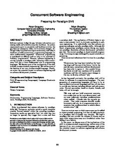
The basic motivation of our research can be illustrated with three images or schemas that are presented in Figures 1.1, 1.2 and 1.3. The first two figures show some texts with several pieces of information decorated in it. If you show such images to a human, he or she will be shortly able to find such pieces of information in any other text of the same kind. But can this relatively simple task do a computer as well? Figure 1.3 represents our first ideas when we started to look for the answer. The figure shows a linguistic tree obtained by automated linguistic analysis of the last sentence of the second figure (Figure 1.2). It already contain lots of indications (decorated with orange tags) of where to look for the wanted piece of information, in this case, the amount of 8,000 Czech Crowns representing the total damage sought by the accident reported in the text. The main motivation for creating our extraction methods was an attempt to use deep linguistic analysis for this task. Especially for the Czech language with free word order this seemed reasonable. It is much more straightforward to design extraction rules on the basis of linguistic dependency trees than to struggle with the surface structure of text. In a dependency tree, the position of a word is determined by its syntactic (analytical trees) or even semantic role (tectogrammatical trees). So the extraction rules might not be dramatically affected by minor variations of the word order. Besides that information extraction and annotation is very interesting and challenging problem, it is also particularly useful. This period can be characterized by information overload and information extraction can provide partial answer to that. It provides fine 1
Figure 1.1: Annotations of Corporate Acquisition Events
fire
started at 3 amateur amateurxunits units Požár byl operačnímu středisku HZS ohlášen dnes ve 2.13 hodin, na místo vyjeli profesionální hasiči ze stanice v Židlochovicích a dobrovolní hasiči z Židlochovic, Žabčic a finished at 3:03 Přísnotic, Oheň, který zasáhl elektroinstalaci u chladícího boxu, hasiči dostali pod kontrolu ve 2.32 hodin a uhasili tři minuty po třetí hodině. Příčinou vzniku požáru byla technická závada, škodu vyšetřovatel předběžně vyčíslil na osm tisíc korun. damage 8 000 CZK id_47443
Figure 1.2: Annotations of Czech Fireman events
id_47443_p1s2 reckon
thousand CZK
damage eight investigating officer …, škodu vyšetřovatel předběžně vyčíslil na osm tisíc korun. …, investigating officer preliminarily reckoned the damage to be 8 000 CZK.
Figure 1.3: Example of a linguistic tree of one analyzed sentence.
2
grained indexing of documents, which supports precise search and document filtering. Navigation within individual documents can be faster and reading can be more effective. Other software programs can use the extracted information and perform additional computations resulting in summaries and answers integrated from different sources. The effort in this direction will hopefully culminate in the realization of the idea of the Semantic Web, when all the information will be available in a machine workable form and the whole (semantic) web could be used as a huge knowledge base.
1.2
Main Contributions
Let us briefly summarize the main contributions of the present work.
1.2.1
New Ideas, Models and Methods
Novel and original approaches or adaptations of existing ones are presented in this work. The extraction method based on manually designed extraction rules is unique in the high expressiveness of extraction rules and the existence GUI (Graphical User Interface) for graphical design of these rules, both of these benefits are brought by the existence of the linguistic tool Netgraph (Section 4.2.4), which was exploited as the core of the extraction method. Very similar approaches to our extraction method based on ILP were already reported in literature, but they were developed partly in parallel with our solution and they do not provide a publicly available and usable implementation. The method also represents the first attempt to use PDT (Prague Dependency Treebank) resources (e.g. tectogrammatical trees, Sections 4.2) in the area of information extraction. Evaluation of the method on the language pair of Czech and English demonstrates its language independence. The topic of shareable extraction ontologies introduces completely new paradigm to the design and usage of extraction ontologies [Embley et al., 2002]. The usage of a semantic web reasoner as the interpreter of an extraction ontology has never been demonstrated before. Last but not least, the attempt to use information extracted from a document for document classification is also reported for the first time, although our attention is more focused on the implementation and evaluation of the Fuzzy ILP Classifier based on the sound theory of fuzzy ILP.
1.2.2
New Software
As a part of our work, new publicly available implementation of the described methods was created. A simple and extensible API (Application Programming Interface) interface of the extraction method based on manually designed extraction rules is provided such that users can design extraction rules in the Netgraph GUI and evaluate them on the whole corpus using this interface. The extraction method based on ILP is fully integrated in GATE (a widely used framework for text engineering; Section 4.5) and it can be used as any other machine learning algorithm inside the framework. Moreover integration of TectoMT linguistic tools (Section 4.2.3) as well as the Netgraph tree viewer (Section 6.2.3) to the GATE framework was realized. Our implementation also provides utility functions for comparative information 3
extraction experiments using the cross-validation technique and investigation of statistical significance. The implementation of the case study with shareable extraction ontologies is not that general as the rest of the software part of our work but it can be easily followed and reproduced in similar experiments. The implementation of the Fuzzy ILP Classifier (Section 6.4) is fully compatible with Weka (a widely used framework for machine learning experiments; Section 4.8) and it can be used as any other Weka classifier, it also provides the possibility of custom integration of the classifier to an existing installation of the Weka system on the user’s computer.
1.2.3 New Data Several new datasets were established as a part of our work. See the complete list of contributed datasets in Section 7.2.1.
1.2.4 Exploitation of Existing Resources Work of other researchers was exploited, extended and/or evaluated in the present work. For example our extraction methods represent the first application of PDT resources (e.g. Netgraph, tectogrammatical trees, etc.) in the area of information extraction. See also the description of experiments performed with the PAUM extraction algorithm (Section 8.2.3), with various semantic web reasoners (Section 8.3.2), Weka classifiers (Section 8.4), etc.
1.2.5 Evaluation Experiments All approaches presented in this thesis were evaluated such that readers can obtain clear picture about the performance and usability of these approaches. Most evaluation experiments are detailed and comprehensive, investigating also the statistical significance of the results.
1.2.6 Publications and New Publicly Available Resources Majority of topics presented in this thesis were already published (going through peer review process), presented and discussed with international audience. Moreover several citations can be found in the literature showing that the work is already contributing to the generally available knowledge. See the complete list of publications in the appendix, Chapter C. Also the software and data parts of our work are publically available on the web, Section 9.6 provides details about the availability of these resources.
1.3 Organization Rather than presenting individual topics or approaches of this thesis separately in distinct chapters, we decided to organize this document according to common aspects of these approaches and to dedicate individual chapters to these aspects instead of approaches. This way, all the (four) topics are described in parallel in each chapter. Chapter 2 provides definitions of the individual problems and consequent tasks solved later in this thesis. Chapter 3 contains description of the most related work of other scientists. Chapter 4 introduces the most important third party tools and resources that 4
were used in our research. Chapter 5 describes solutions, used models and methods of the individual approaches presented in this thesis. Chapter 6 provides details about implementation of all the approaches. Chapter 7 describes all datasets that were used in our experiments. Chapter 8 describes all experiments that we performed mostly for evaluation of the approaches. Finally, Chapter 9 concludes the thesis.
5
6
2. Problems and Consequent Tasks Definitions As already said in introduction, four separate topics are presented in this thesis. This chapter provides definitions of the main problems connected with these topics and consequent tasks that have to be addressed to solve these problems.
2.1 2.1.1
Information Extraction The Problem
The basic problem addressed by information extraction approaches can be formulated as follows. We have a large collection of texts (or a source of texts) and we want to have a machine readable (understandable, workable) or structured form of the information present in these texts. Why? Because additional postprocessing of the information is needed. Let us for example have texts about acquisition events. Each text describes a single acquisition event and answers to following questions can be found in these texts. • What was the object of the acquisition? • Who was the buyer? • What was the deal amount? • What was the acquisition date? If we put the corresponding information into a relational table then we can easily obtain statistics like numbers of acquisitions per month or a list of ten most valuable (largest deal amount) acquired subjects, etc. This would be impossible if the information was kept in the textual form only. Document search and indexing is another important purpose of information extraction. Let us imagine a person interested in articles about acquisitions made in January 2009 where the deal amount was between 100 and 500 million dollars. Keyword search and indexing can not satisfy this need accurately. But if we have corresponding machine readable information, it is easy to create a simple search engine supporting this kind of queries. The idea of the Semantic Web [Berners-Lee et al., 2001] brings us to even a bigger problem that could be partly solved by information extraction approaches. On the Semantic Web, as much information as possible should be in a structured machine readable form. But absolute majority of ordinary content of the present day web is understandable only for humans. Machines can use only very limited part of the present day web. This issue is often called “Semantic Web Bottleneck” [Konstantinou et al., 2010].
2.1.2
Consequent Tasks
The definition of the problem presented in the previous section was general. We did not specify any particular kind of information to be extracted or target structure for capturing it. This is exactly the point, where different kinds of information extraction approaches differ. Currently, the variety of information extraction approaches is huge. In this thesis, we will focus on a small subset only. 7
It was already mentioned in the previous section that the source information is captured as text. Let us specify it more precisely: We are interested in cases where information is expressed in plain text in natural language. We do not consider additional structural information or formatting instructions that may be potentially available e.g. through HTML or XML tags. We are primarily interested in texts consisting of natural language sentences. We do not consider textual fragments, tables, etc. These two options were selected mainly based on our personal interest and background. This setting is very close to the topic of natural language understanding, very attractive problem since the very establishment of artificial intelligence1 . And this setting is also very common in practice, e.g. in news articles, scientific papers, blog posts, official statements and reports, offers, requests, advertisements, etc. After the specification of input format, let us specify the kind of information to be extracted and the target structure for capturing it. Higher complexity of the extracted information makes the task more difficult. The entire complexity of human language is still far beyond the boundary of machine workability. In practice, extraction of very simple facts represented by plain relations already provides significant help. For example only one relation (e.g. “acquisition”) with four arguments (“object”, “buyer”, “deal amount” and “date”) would be sufficient for capturing the information about acquisition events mentioned above. In this thesis, we concentrate on these simple relational facts, not considering any of the wide range of possibilities that the human language offers like expression of tense, causality, modality, general statements with quantifiers, etc. Stating that we will extract “simple relational facts” is still not precise enough and several well established information extraction tasks conform to this statement. We will describe them in Sections 2.1.4–2.1.8, but before that, it is necessary to explain how the term “document annotation” will be used in this thesis.
2.1.3 Document Annotation Document Annotation is a term, which usually refers to the process of putting annotations to a document. In this thesis, the term annotations will always refer to a special kind of annotations used in the GATE framework. These annotations refer to (usually shorter) segments of text and they provide a label (or annotation type) and arbitrary set of features to each such segment (or simply annotation). Each annotation occupies a continuous portion of text between the beginning and the end of the annotation. These annotations can be easily visualized using colored background in text. Different annotation types are usually decorated with different colors; see Figure 1.1 for an example. Section 4.5.1 provides some technical details about this kind of annotations. There is a very small difference between the process of document annotation and information extraction. In fact they are equivalent in the case we are describing. Because annotations can be reconstructed from extracted relational facts and relational facts can be reconstructed from annotations. There are only two conditions that have to hold true: (1) It has to be always possible to determine the portion of text representing any extracted fact. (2) Each annotation has to keep all its relational arguments as annotation features. Relation name can be saved as annotation label and vice versa.
1
See e.g. the history part of the Wikipedia article Natural language understanding: http://en. wikipedia.org/wiki/Natural_language_understanding#History
8
2.1.4
Entity Recognition
Entity Recognition or Named Entity Recognition corresponds to the extraction task of identification of significant entities (people, organizations, locations, chemicals, genes, etc.) that are present in text. From the annotation perspective, this is the simplest annotation task: just to mark these entities in text and assign correct labels to them. From the relational perspective, this task corresponds with unary relation extraction. It can be for example illustrated on following sentence: Google just announced that it is acquiring Motorola Mobility. There are two entities mentioned in this sentence: Google and Motorola Mobility. Both entities have to be extracted and put into correct unary relations, e.g. “organization(Google)” or “company(Google)” depending on the used vocabulary. Or, in the annotation case, they have to be marked in text and annotated with corresponding label (“organization” or “company”).
2.1.5
Relation Extraction
Relation Extraction is an extraction task that usually comes after entity recognition. When all the significant entities are identified, the task is to connect together those entities that are connected in text and to assign the correct label (relation name) to this connection. Let us again use the example sentence about Google acquiring Motorola. The extracted relation should be connecting the two entities (in the right order) and the label would be something like: “acquiredBy”, “purchasing” or “takingOver” (depending on the system vocabulary; note the dependency between the label and the relation orientation.)
2.1.6
Event Extraction
In literature, Relation Extraction usually refers to binary relations only and Event Extraction is used for relations (events) with more arguments. Individual events have to be correctly identified in text and arguments have to be assigned to them in proper roles. For example an acquisition event can have roles like purchaser, seller, acquired, deal amount, etc. We have to extend our running example with Google and Motorola to demonstrate event extraction on it: Google just announced that it is acquiring Motorola Mobility. The search and online advertising company is buying the company for approximately $12.5 billion (or $40 per share), in cash. In this case, both sentences would be covered by the acquisition event with attached arguments: purchaser(Google), acquired(Motorola Mobility) and deal_amount($12.5 billion).
2.1.7
Event Extraction Encoded as Entity Recognition
In practice, there are quite common cases when only a single event is reported in each document. In this case it is not necessary to annotate the exact location of the event in the document and mere identification of event roles is sufficient. Technically, annotation of such events looks like the same as annotation of ordinary entities of an entity recognition 9
task. The difference is only in labels of these entities because they correspond with event roles. A proper example would look like a combination of the examples that we have used for the demonstration of Entity Recognition and Event Extraction tasks. Google, Motorola and ‘$12.5 billion’ will be annotated the same as in Event Extraction – purchaser(Google), acquired(Motorola Mobility), deal_amount($12.5 billion) – but they will be not linked to any particular event because they belong to the implicit event identified by the current document. Both manually annotated datasets described in this thesis are of this kind of event extraction; see details in Sections 7.3.2 and 7.3.3.
2.1.8 Instance Resolution Instance Resolution further extends entity recognition. It aims at linking a particular entity to its unique representative (or identifier) such that the same entities have always the same identifier and, vice versa, different entities have always different identifiers. Disambiguation is the main task that has to be solved by instance resolution. It can be illustrated on some ambiguous entity, for example “George Bush”. General entity recognition system just marks it in text and assigns a corresponding label (e.g. person, politician or president – depending on the granularity of the system) to it. In extraction case, such system just puts the string into the corresponding relation. Instance resolution is more difficult. Instance resolution system has to select the right representative for that entity – George W. Bush (junior) or George H. W. Bush (senior) that will be probably both available in the system’s database. Similarly, instance resolution system has to assign the same identifier in cases where for example shortcuts are used, e.g. “George W. Bush” and “G. W. Bush” should be linked to the same identifier.
2.1.9 Summary The problem of information extraction consists in obtaining machine workable form of information that was previously available in textual form only. We have specified that we are interested only in extraction of simple relational facts and that the extracted facts can be kept either as relational data or they can be of the form of document annotations. Depending on the complexity of extracted information, four basic extraction tasks were defined: • Entity Recognition, • Relation Extraction, • Event Extraction and • Instance Resolution.
2.2 Machine Learning for Information Extraction 2.2.1 The Problem Development of an information extraction system is always, more or less, dependent on a concrete domain and extraction tasks. It is always necessary to adapt the system when it should be used in a new domain with new extraction tasks. The difficulty of such adaptation 10
varies. In some cases the whole system has to be redesigned and reimplemented. Many systems are based on some kind of extraction rules or extraction models and only these rules or models have to be adapted in such case. But still, only highly qualified experts can do such adaptation. These experts have to know the extraction system in detail as well as the domain, target data (texts) and extraction tasks. Such qualification is sometimes (e.g. in biomedical domains) unreachable in one person and difficult cooperation of a domain expert with a system expert is necessary.
2.2.2
Consequent Tasks
Usage of machine learning techniques can address this problem in such a way that the system is capable to adapt itself. But a learning collection of example texts with gold standard annotations has to be provided. The effort needed to build such collection is still demanding, but such gold standard collection is not dependent on any concrete extraction system and expert knowledge related to extraction systems is not needed for its construction. Another important purpose of machine learning is that extraction rules or models constructed by machine learning techniques are often more successful than those designed manually.
2.3
Extraction Ontologies
2.3.1
The Problem
Information extraction and automated semantic annotation of text are usually done by complex systems and all these systems use some kind of model that represents the actual task and its solution. The model is usually represented as a set of some kind of extraction rules (e.g., regular expressions), gazetteer lists2 or it is based on some statistical measurements and probability assertions (classification algorithms like Support Vector Machines (SVM), Maximum Entropy Models, Decision Trees, Hidden Markov Models (HMM), Conditional Random Fields (CRF), etc.) Before the first usage of an information extraction system, such model is either created by a human designer or it is learned from training dataset. Then, in the actual extraction/annotation process, the model is used as a configuration or as a parameter of the particular extraction/annotation system. These models are usually stored in proprietary formats and they are accessible only by the corresponding extraction system. In the environment of the Semantic Web it is essential that information is shareable and some ontology based IE systems keep the model in so called extraction ontologies [Embley et al., 2002]. Extraction ontologies should serve as a wrapper for documents of a narrow domain of interest. When we apply an extraction ontology to a document, the ontology identifies objects and relationships present in the document and it associates them with the corresponding ontology terms and thus wraps the document so that it is understandable in terms of the ontology [Embley et al., 2002]. In practice, the extraction ontologies are usually strongly dependent on a particular extraction/annotation system and cannot be used separately. The strong dependency of 2
See Section 4.5.2 for details about the term gazetteer list.
11
an extraction ontology on the corresponding system makes it very difficult to share. When an extraction ontology cannot be used outside the system there is also no need to keep such “ontology” in a standard ontology format (RDF or OWL).
2.3.2 Consequent Tasks The cause of the problem is that a particular extraction model can be only used and interpreted by the corresponding extraction tool. If an extraction ontology should be shareable, there has to be a commonly used tool, which is able to interpret the extraction model encoded by the extraction ontology. For example Semantic Web reasoners can play the role of commonly used tools that can interpret shareable extraction ontologies. Although it is probably always possible to encode an extraction model using a standard ontology language, only certain way of encoding makes it possible to interpret such model by a standard reasoner in the same way as if the original extraction tool was used. The difference is in semantics. It is not sufficient to encode just the model’s data, it is also necessary to encode the semantics of the model. Only then the reasoner is able to interpret the model in the same way as the original tool. If the process of information extraction or semantic annotation should be performed by an ordinary Semantic Web reasoner then only means of semantic web inference are available and the extraction process must be correspondingly described.
2.4 Document Classification 2.4.1 The Problem Similarly to information extraction, document classification solves a problem when we have a large collection of documents and we do not exactly know what the individual documents are about. Document classification helps in cases when we want to just pick such documents that belong to certain category, e.g. to pick only football news from a general collection of sport news articles.
2.4.2 Consequent Tasks The task of document classification can be formulated as follows. Having a textual document and a (usually small) set of target categories, the task is to decide to which category the document belongs. In the case of the present thesis, we are especially interested in cases when the set of categories is ordered or, in other words, we can always decide which one of any two categories is higher. This kind of categories often corresponds with some ranking and individual categories then correspond to ranking degrees, e.g. ranking of seriousness of a traffic accident, which is used in classification experiments of the present thesis (see the Seriousness Ranking part of Section 7.3.6).
12
3. Related Work This chapter shortly introduces mostly related work of other researchers. The chapter is split to three main sections. Section 3.1 is dedicated to information extraction approaches, Section 3.2 to extraction ontologies and Section 3.3 to document classification.
3.1
Information Extraction Approaches
3.1.1
Deep Linguistic Parsing and Information Extraction
The choice of the actual learning algorithm depends on the type of structural information available. For example, deep syntactic information provided by current parsers for new types of corpora such as biomedical text is seldom reliable, since most parsers have been trained on different types of narrative. If reliable syntactic information is lacking, sequences of words around and between the two entities can be used as alternative useful discriminators. [Bunescu, 2007] Since that time, the situation has improved and deep linguistic parsing is often used even for biomedical texts (because new biomedical corpora are available for retraining of the parsers; see e.g. in [Buyko and Hahn, 2010]) and dependency graphs constitute the fundamental data structure for syntactic structuring and subsequent knowledge extraction from natural language documents in many contemporary approaches to information extraction (see details about individual information extraction systems in Section 3.1.2). Currently, quite a lot of parsers can be used for generation of syntactic dependency structures from natural language texts. Some of them will be briefly described in Section 4.2.1. Besides the possibility of using different parsers there are also various language dependency representations (LDR) such as the Stanford [de Marneffe et al., 2006] and CoNLL-X [Johansson and Nugues, 2007] dependencies and the Functional Generative Description (FGD) [Sgall et al., 1986] studied mainly in Prague. All the dependency representations are very similar from the structural point of view; they differ mainly in the number of different dependency kinds they offer. FGD provides also additional node attributes and so called layered approach (see in Section 4.1) and is the only representation available for Czech. It is also worthy to investigate the impact of usage of different LDRs on the performance of information extraction. Buyko and Hahn [2010] compared the impact of different LDRs and parsers in their IE system, namely Stanford and CoNLL-X dependencies and usage of different trimming operations. Their findings are definitely not supporting one choice against another because one representation was better for some tasks and another one for other tasks, see examples in their paper. More important seems to be the quality of used parser.
3.1.2
IE Systems Based on Deep Language Parsing
We describe in this section several information extraction systems based on deep language parsing. The systems differ greatly in the manner of using LDR. 13
Rule Based Systems There are many systems using hand crafted extraction rules based on LDR. These systems need assistance from a human expert that is able to design the extraction rules manually. The advantage of these systems is that there is no need of learning (or training) data collection. For example Fundel et al. [2007] used a simple set of rules and the Stanford parser1 for biomedical relation extraction. Shallow and deep parsers were used by Yakushiji et al. [2001] in combination with mapping rules from linguistic expressions to biomedical events. Classical Machine Learning Systems Classical machine learning (ML) approaches rely on the existence of a learning collection. They usually use LDR just for construction of learning features for propositional learners like decision trees, neural networks, SVM, etc. Learning features are selected manually when the system is being adapted to new domain or extraction task. For example in [Bunescu and Mooney, 2007], learning features based on so called dependency paths constructed from LDR are used for relation extraction. Similar approach was used in [Buyko et al., 2009] for biomedical event extraction. [Li et al., 2009] described machine learning facilities available in GATE. This approach is an example of classical adaptation of propositional learners for information extraction, but it is not necessarily connected with LDR. GATE itself does not provide any prebuilt functions for working with LDR but they can be added as they were in our case (see in Section 6.2.2). Inductive Systems There are also systems using some inductive technique e.g. Inductive Logic Programming (ILP, see also Section 4.7) to induce learning features or extraction rules automatically from learning collection. In these cases it is neither necessary to manually design extraction rules nor select the right learning features. For example Ramakrishnan et al. [2007] used the dependency parser MINIPAR2 [Lin, 2003] and ILP for construction of both: 1. learning features for SVM classifier and 2. plain extraction rules. They compared the success of the two approaches and discovered that the extraction model constructed by SVM (based on the induced learning features) was more successful than the plain extraction rules directly constructed by ILP. Similarity Based Systems Several information extraction related systems do some kind of similarity search based on the syntactic structure. For example Etzioni et al. [2008] designed a data-driven extraction system performing a single-pass-over-a-corpus extraction of a large set of relational tuples without requiring any human input (e.g. without the definition of extraction tasks). And for example Wang and Neumann [2007] used syntactic structure similarity for textual entailment. 1 2
http://nlp.stanford.edu/software/lex-parser.shtml http://webdocs.cs.ualberta.ca/~lindek/minipar.htm
14
3.1.3
Inductive Logic Programming and Information Extraction
There are many users of ILP in the linguistic and information extraction area. For example Konstantopoulos [2003] used ILP for shallow parsing and phonotactics. Junker et al. [1999] summarized some basic principles of using ILP for learning from text without any linguistic preprocessing. One of the most related approaches to ours was described by Aitken [2002]. The authors use ILP for extraction of information about chemical compounds and other concepts related to global warming and they try to express the extracted information in terms of ontology. They use only the part of speech analysis and named entity recognition in the preprocessing step. But their inductive procedure uses also additional domain knowledge for the extraction. Ramakrishnan et al. [2007] used ILP to construct good features for propositional learners like SVM to do information extraction. It was discovered that this approach is a little bit more successful than a direct use of ILP but it is also more complicated. The later two approaches could be also employed in our solution.
3.1.4
Directly Comparable Systems
Thanks to the fact that evaluation of our extraction method based on ILP was performed also on a commonly used dataset, its performance can be compared with other information extraction systems that were evaluated on the dataset as well. Details about the results of the comparison will be presented in Section 8.2.6. Brief introduction of the directly comparable systems will be present in this section. PAUM The PAUM (Perceptron Algorithm with Uneven Margins) algorithm [Li et al., 2002] is one of machine learning alternatives provided by GATE. The algorithm represents a slight modification of the classical Perceptron [Rosenblatt, 1957] used in neural networks and extended by SVM [Cortes and Vapnik, 1995]. PAUM belongs to the category of classical propositional learners working on a set of learning features manually extracted from text. Thanks to the easy accessibility of PAUM in GATE, all our machine learning experiments could be performed with PAUM in the same time as our extraction method based on ILP. Hence these two methods were directly compared with absolutely equal conditions (the same learning and evaluation sets) and statistically significant results were recorded; see the details in Section 8.2. SRV SRV [Freitag, 1999] is a rule induction extraction system working on a set of learning features; extensible set of features is predefined allowing quick porting to novel domains. Chang et al. [2006] provided a great and concise description of SRV in their survey article: SRV is a top-down relational algorithm that generates single-slot extraction rules. It regards IE as a kind of classification problem. The input documents are tokenized and all substrings of continuous tokens (i.e. text fragments) are labeled as either extraction target (positive examples) or not (negative examples). The rules generated by SRV are logic rules that rely on a set of token-oriented features (or predicates). These features have two basic varieties: simple and relational. A simple feature is a function that maps a token into some discrete value such as length, character type (e.g., numeric), orthography (e.g., capitalized) and part of speech (e.g., verb). A relational feature maps 15
a token to another token, e.g. the contextual (previous or next) tokens of the input tokens. The learning algorithm proceeds as FOIL [Quinlan, 1990], starting with entire set of examples and adds predicates greedily to cover as many positive examples and as few negative examples as possible. Freitag [1999] experimented with the usage of WordNet [Miller, 1995] and the link grammar parser [Sleator and Temperley, 1993]. Surprisingly most of the extraction performance was achieved with only the simplest of information, without the usage of the linguistic resources. HMM Freitag and McCallum [1999] described how Hidden Markov Models can be successfully applied to information extraction. They used a statistical technique called shrinkage for balancing the trade-of between the complexity of models and small quantifies of available training data. The combination of shrinkage with appropriately designed topologies yields a learning algorithm comparable with the state of the art systems. The authors do not report usage of any additional linguistic resources like WordNet, POS tagger or syntactical parser. Elie Elie [Finn and Kushmerick, 2004] is another representative of a classical propositional learner working on a set of learning features manually extracted from text. Finn and Kushmerick [2004] show that the use of an off-the-shelf support vector machines implementation is competitive with current IE algorithms and that their “multilevel boundary classification” approach outperforms current IE algorithms on a variety of benchmark tasks. The multilevel boundary classification approach consists in a combination of the predictions of two sets of classifiers, one set (L1) with high precision and one (L2) with high recall. The L1 classifiers adopt the the standard “IE as classification” approach. L2 uses a second level of “biased” classifiers trained only on surrounding tokens of positive learning instances. The authors used Brill’s POS tagger [Brill, 1994] providing, apart from POSs, also chunking information (noun-phrases, verb-phrases) about the tokes. Their second resource was a gazetteer list containing U.S. fist-names and last-names, list of countries, cities, streets, titles, etc. See the details in their paper. SVM with ILP Feature Induction We already mentioned the work of Ramakrishnan et al. [2007] in previous sections. Once because they used deep language parsing (MINIPAR parser [Lin, 2003]) and once because they used ILP. Their approach is very close to ours and it is even more complex. Instead of using ILP directly for the construction of extraction rules, they used ILP just for construction of good learning features for SVM classifier. They also used WordNet as a source of additional information. Surprising fact about their solution is that it was not that much successful as one would expect (see the results in Section 8.2.6), especially when compared with the relatively simple solution of the PAUM algorithm that we have been experimenting with. It could be caused by the usage of different version of the dataset or by too large number of learning features (the authors reported up to 20,000 learning features). 16
3.1.5
Semantic Annotation
Last category of related work goes in the direction of semantics and ontologies. Bontcheva et al. [2004] described ontology features in GATE. They can be easily used to populate an ontology with extracted data. We discus this topic later in Section 5.2.6. See also references to related work connected with ontologies and information extraction in the following section.
3.2
Extraction Ontologies
Ontology-based Information Extraction (OBIE) [Wimalasuriya and Dou, 2010] or Ontologydriven Information Extraction [Yildiz and Miksch, 2007] has recently emerged as a subfield of information extraction. Furthermore, Web Information Extraction [Chang et al., 2006] is a closely related discipline. Many extraction and annotation tools can be found in the above mentioned surveys (Chang et al. [2006]). Many of the tools also use an ontology as the output format, but almost all of them store their extraction models in proprietary formats and the models are accessible only by the corresponding tool. In the literature, we have found only two approaches that use extraction ontologies. The former one was published by D. Embley [Embley et al., 2002; Embley, 2004] and the later one – IE system Ex3 was developped by M. Labský [Labský et al., 2009]. But in both cases the extraction ontologies are dependent on the particular tool and they are kept in XML files with a proprietary structure. By contrast Wimalasuriya and Dou [2010] (a recent survey of OBIE systems) do not agree with allowing for extraction rules to be a part of an ontology. They use two arguments against that: 1. Extraction rules are known to contain errors (because they are never 100% accurate), and objections can be raised on their inclusion in ontologies in terms of formality and accuracy. 2. It is hard to argue that linguistic extraction rules should be considered a part of an ontology while information extractors based on other IE techniques (such as SVM, HMM, CRF, etc. classifiers used to identify instances of a class when classification is used as the IE technique) should be kept out of it: all IE techniques perform the same task with comparable effectiveness (generally successful but not 100% accurate). But the techniques advocated for the inclusion of linguistic rules in ontologies cannot accommodate such IE techniques. The authors then conclude that either all information extractors (that use different IE techniques) should be included in the ontologies or none should be included. Concerning the first argument, we have to take into account that extraction ontologies are not ordinary ontologies, it should be agreed that they do not contain 100% accurate knowledge. The estimated accuracy of the extraction rules can be saved in the extraction ontology and it can then help potential users to decide how much they will trust the extraction ontology. Concerning the second argument, we agree that in the case of complex classification based models (SVM, HMM, CRF, etc.) serialization of such model to RDF does not make much sense (cf. Section 2.3.2). But on the other hand we think that there are cases 3
http://eso.vse.cz/~labsky/ex/
17
when (shareable) extraction ontologies can be useful and in the context of Linked Data4 providing shareable descriptions of information extraction rules may be valuable. It is also possible that new standard ways how to encode such models to an ontology will appear in the future. Let us briefly remind main ontology definitions because they are touched and in a sense misused in our work on shareable extraction ontologies. The most widely agreed definitions of an ontology emphasize the shared aspect of ontologies: An ontology is a formal specification of a shared conceptualization. [Borst, 1997] An ontology is a formal, explicit specification of a shared conceptualization. [Studer et al., 1998] Of course the word ‘shareable’ has different meaning from ‘shared’. (Something that is shareable is not necessarily shared, but on the other hand something that is shared should be shareable.) We do not think that shareable extraction ontologies will contain shared knowledge about how to extract data from documents in certain domain. This is for example not true for all extraction models artificially learned from a training corpus. Here shareable simply means that the extraction rules can be shared amongst software agents and can be used separately from the original tool. This is the deviation in use of the term ‘ontology’ in the context of (shareable) extraction ontologies (similarly for “document ontologies”, see in Section 5.3.1).
3.3 Document Classification 3.3.1 General Document Classification There are plenty of systems dealing with text mining and text classification. Reformat et al. [2008] use ontology modeling to enhance text identification. Chong et al. [2005] use preprocessed data from National Automotive Sampling System and test various soft computing methods to model severity of injuries (some hybrid methods showed best performance). Methods of Information Retrieval (IR) are numerous, mainly based on key word search and similarities. The Connection of IR and text mining techniques with web information retrieval can be found in the chapter “Opinion Mining” in the book of Bing Liu [2007].
3.3.2 ML Classification with Monotonicity Constraint The Fuzzy ILP Classifier can be seen as an ordinary classifier for data with the monotonicity constraint (the target class attribute has to be monotonizable – a natural ordering has to exist for the target class attribute). There are several other approaches addressing the classification problems with the monotonicity constraint. The CART-like algorithm for decision tree construction does not guarantee a resulting monotone tree even on a monotone dataset. The algorithm can be modified [Bioch and Popova, 2009] to provide a monotone tree on the dataset by adding the corner elements of a node with an appropriate class label to the existing data whenever necessary. 4
http://linkeddata.org/
18
An interesting approach was presented by Kotlowski and Slowinski [2009]: first, the dataset is “corrected” to be monotone (a minimal number of target class labels is changed to get a monotone dataset), then a learning algorithm (linear programming boosting in the cited paper) is applied. Several other approaches to monotone classification have been presented, including instance based learning [Lievens et al., 2008] and rough sets [Bioch and Popova, 2000].
19
20
4. Third Party Tools and Resources In our solution we have exploited several tools and formalisms. They can be divided into two groups: linguistics and (inductive) logic programming. First we describe the linguistic tools and formalisms, the rest will follow.
4.1
Prague Dependency Treebank (PDT)
There exist several projects1 closely related to the “Prague school of dependency linguistics’’ and the Institute of Formal and Applied Linguistics2 in Prague, Czech Republic (ÚFAL). All the projects share common methodology and principles concerning the formal representation of natural language based on the theory of Functional Generative Description (FGD) [Sgall et al., 1986]. FGD provides a formal framework for natural language representation. It is viewed as a system of layers (stratification) expressing the relations of forms and functions. Special attention is devoted to the layers of language meaning described inter alia in dependency terms. We will refer to these principles and related formalism as “PDT principles and formalisms’’ in the present work because the PDT projects are the most fundamental and the elaborate annotation guidelines (see bellow) were compiled within these projects. The most relevant principles for the present work will be briefly described in this section.
4.1.1
Layers of Dependency Analysis in PDT
Unlike the usual approaches to the description of English syntax, the Czech syntactic descriptions are dependency-based, which means that every edge of a syntactic tree captures the relation of dependency between a governor and its dependent node. In PDT, text is split into individual sentences and dependency trees are built form them. Nodes of the trees are represented by individual words or tokens and edges represent their linguistic dependencies (simplified speaking, see bellow). Among others, two most important kinds of dependencies are distinguished: syntactical dependencies and “underlying (deep) structure’’ dependencies. Syntactical dependencies are often called analytical and the latter are called tectogrammatical dependencies. These two kinds of dependencies form two kinds of dependency trees: analytical trees and tectogrammatical trees. The situation is usually described using the concept of different layers (or levels) of annotation. It is illustrated by Figure 4.1. We can start the description at the bottom of the picture: There is the surface structure of the sentence (w-layer) which represent the raw text without any modifications and annotations and is not considered as a layer of annotation (it can even preserve spelling errors, see e.g. the missing space between words ‘do’ and ‘lesa’ (into forest) in the example sentence, Figure 4.1). The lowest level of linguistic annotation (m-layer) represents morphology. Word forms are disambiguated and correct lemmas (dictionary form) and morphological tags are assigned at this level. The second level of annotation is called analytical (a-layer). At this level the syntactical dependencies of words are captured (e.g. subject, predicate, object, attribute, adverbial, etc.) The top level of annotation is called tectogrammatical (t-layer), sometimes also called “layer of deep syntax”. At this level some tokens (e.g. tokens without lexical meaning) are leaved 1
Prague Dependency Treebank (PDT 1.0, PDT 2.0 [Hajič et al., 2006]), Prague English Dependency Treebank (PEDT 1.0), Prague Czech-English Dependency Treebank (PCEDT 1.0) 2 http://ufal.mff.cuni.cz
21
out or “merged’’ together (e.g. prepositions are merged with referred words). Also some nodes without a morphological level counterpart are inserted to the tectogrammatical tree at certain occasions (e.g. a node representing omitted subject – on Figure 4.1 labeled as “#PersPron’’). More over all the layers are interconnected and additional linguistic features are assigned to tree nodes. Among others: morphological tag and lemma is assigned at the morphological level; analytical function (the actual kind of the particular analytical dependency, e.g. predicate, subject, object, etc.) is assigned to dependent nodes at the analytical level; semantic parts of speech + grammatemes (e.g. definite quantificational semantic noun (n.quant.def) + number and gender, etc.) and tectogrammatical functor (e.g. actor (ACT), patient (PAT), addressee (ADDR), temporal: when (TWHEN), directional: to (DIR3), etc.) is assigned at the tectogrammatical level. Detailed information can be found: • Homepage of the PDT 2.0 project: http://ufal.mff.cuni.cz/pdt2.0/ • Annotation guidelines: – Morphological Layer Annotation [Zeman et al., 2005] – Analytical Layer Annotation [Hajičová et al., 1999] – Tectogrammatical Layer Annotation [Mikulová et al., 2006] – Tectogrammatical Layer Annotation for English (PEDT 1.0) [Cinková et al., 2006]
4.1.2 Why Tectogrammatical Dependencies? The practice has shown that representing only syntactical roles of tokens present in a sentence is not sufficient to capture the actual meaning of the sentence. Therefore the tectogrammatical level of representation was established. Or according to Klimeš [2006]: Annotation of a sentence at this [tectogrammatical] layer is closer to meaning of the sentence than its syntactic annotation and thus information captured at the tectogrammatical layer is crucial for machine understanding of a natural language. This can be used in areas such as machine translation and information retrieval, however it can help other tasks as well, e.g. text synthesis. One important thing about t-layer is that it is designed as unambiguous from the viewpoint of language meaning [Sgall et al., 1986], which means that synonymous sentences should have the same single representation on t-layer. Obviously this property is very beneficial to information extraction because t-layer provides certain generalization of synonymous phrases and extraction techniques do not have to handle so many irregularities.
4.2 PDT Tools and Resources In this section several linguistic tools and resources that are being developed at ÚFAL will be described. These tools and resources are closely connected with the PDT projects and they have been used also in the present work for various purposes. 22
Sample sentence (in Czech): English translation (lit.): [He]
Byl by šel dolesa. would have gone intoforest.
Figure 4.1: Layers of linguistic annotation in PDT
23
4.2.1 Linguistics Analysis Linguistic tools that were used for automated (machine) linguistic annotations of texts will be briefly described in this section. These tools are used as a processing chain and at the end of the chain they produce tectogrammatical dependency trees. Tokenization and Segmentation On the beginning of text analysis the input text is divided into tokens (words and punctuation); this is called tokenization. Sequences of tokens are then (or simultaneously) divided into sentences; this is called segmentation. Note that although the task seems quite simple, especially segmentation is not trivial and painful errors occur at this early stage e.g. caused by abbreviations ended by full stop in the middle of a sentence. There are several tools available for Czech and English. The oldest (Czech) one can be found on the PDT 2.0 CD-ROM Hajič et al. [2006] and several choices are provided by TectoMT (see Section 4.2.3) and GATE (see Section 4.5). The best choice for Czech is probably TextSeg [Češka, 2006], which is available through TectoMT. Morphological Analysis Because Czech is a language with rich inflections, morphological analysis (or at least lemmatization) is an important means to success of any NLP task (starting with key word search and indexing.) In PDT, morphological analysis is a necessary precondition for analytical analysis (next section). The task of morphological analysis is for given word form in given context to select the right pair of lemma (dictionary form) and morphological tag. In PDT, the tag includes part of speech (POS) and other linguistic categories like gender, number, grammatical case, tense, etc., see morphological annotation guidelines for details. For Czech two main tools are available: Feature-based tagger3 by Hajič [2000] and perceptron-based tagger Morče4 by Votrubec [2006]. Morče is several years newer and it achieved few points better accuracy on PDT 2.0 (94.04% vs. 95.12% see in [Spoustová et al., 2007]). Both tools are available through TectoMT, Morče also for English. Analytical Analysis The task of Analytical analysis is to build up a syntactical dependency tree (analytical tree) from a morphologically analyzed sentence and to assign the right kind of dependency (analytical function) to every edge of the tree. There were experiments with almost all well known parsers on the Czech PDT data5 . But two of them have proven themselves in practice: Czech adaptation of Collins’ parser [Collins et al., 1999] and Czech adaptation of McDonald’s MST parser [Novák and Žabokrtsky, 2007]. Again the second tool is few years newer and few points better in accuracy (80.9% vs. 84.7% on PDT 2.05 ). The Collins’ parser can be found on the PDT 2.0 CD-ROM and the MST parser is available through TectoMT. The analytical analysis of English is not very well established because PEDT 1.06 contains only tectogrammatical level of annotation and there is no other English treebank 3
http://ufal.mff.cuni.cz/tools.html/fbtag.html http://ufal.mff.cuni.cz/morce/ 5 See details at http://ufal.mff.cuni.cz/czech-parsing/ 6 http://ufal.mff.cuni.cz/pedt/ 4
24
for the analytical level. The English analytical analysis is regarded rather as a part of English tectogrammatical analysis; see details in [Klimeš, 2007]. Tectogrammatical Analysis During tectogrammatical analysis analytical trees are transformed to tectogrammatical ones. Merging, omitting and inserting of tree nodes takes place as well as assignment of all the complex linguistic information of the tectogrammatical level (semantic parts of speech, grammatemes, tectogrammatical functors, etc.) The tectogrammatical analysis can by performed by a variety of TectoMT blocks (depending on the amount of requested linguistic information, for example only tectogrammatical functors can be assigned.) Better results can be obtained through transformation-based tools developed by Václav Klimeš: [Klimeš, 2006] for Czech and [Klimeš, 2007] for English; they are also available through TectoMT.
4.2.2
Tree Editor TrEd, Btred
TrEd is the ÚFAL key tool for work with dependency based linguistic annotations. It provides a comfortable GUI for navigation, viewing and editing of linguistic trees at different levels of annotation, for different languages and different treebank schemas. TrEd is implemented in Perl and it is available for a variety of platforms (Windows, Unix, Linux, Mac OS X). Homepage of the project: http://ufal.mff.cuni.cz/~pajas/tred/ Btred TrEd can be also controlled using a powerful set of Perl macros and there is also a noninteractive version of TrEd called Btred, which allows batch evaluation of user macros on an arbitrary set of annotated documents. Btred/ntred tutorial: http://ufal.mff.cuni.cz/~pajas/tred/bn-tutorial.html PML Tree Query PML Tree Query (PML-TQ) [Pajas and Štěpánek, 2009] is a TrEd based module for searching through a treebank using a complex tree based query language. It is a new alternative for Netgraph (Section 4.2.4). Homepage of the project: http://ufal.mff.cuni.cz/~pajas/pmltq/
4.2.3
TectoMT
TectoMT [Žabokrtský et al., 2008] is a Czech project that contains many linguistic tools for different languages including Czech and English; all the tools are based on the dependency based linguistic theory and formalism of PDT. It is implemented in Perl; highly exploiting TrEd libraries. The recommended platform is Linux. It is primarily aimed at machine translation but it can also facilitate development of software solutions of other NLP tasks. We have used a majority of applicable tools from TectoMT (e.g. tokeniser, sentence splitter, morphological, analytical and tectogrammatical analyzers for Czech and English). We have also developed TectoMT wrapper for GATE, which makes it possible to use TectoMT tools inside GATE, see details in Section 6.2.1. 25
Similarly to GATE, TectoMT supports building of application pipelines (scenarios) composed of so called blocks – processing units responsible for single independent task (like tokenization, parsing, etc.) Homepage of the project: or more recent one:
http://ufal.mff.cuni.cz/tectomt/ http://ufal.mff.cuni.cz/treex/
4.2.4 Netgraph Netgraph [Mírovský, 2006] is a linguistic tool used for searching through a syntactically annotated corpus of a natural language (corpus of linguistic dependency trees). Besides the searching capabilities it also provides a GUI for viewing of dependency trees. Both of these features were exploited in the present work. Netgraph implementation is client-server based and a special query language is used for searching. The query language allows putting restrictions on the shape of a tree and on values of attributes of an arbitrary tree node. Besides that nodes of a query can be marked as optional (not necessarily present in a matching tree) and names can be assigned to query nodes. Naming of query nodes allows putting restrictions based on referenced nodes (Give me all trees where there is a node with two children and both children have the same lemma.) See also Section 6.1.2, it provides additional information about the query language including example Netgraph queries. Currently, Netgraph is replaced by PML Tree Query (Section 4.2.2) and the Netgraph development is “discontinued”. We use Netgraph in the present work because PML Tree Query is quite young and it was not available when our development started and because Netgraph is written in Java, the language used for GATE as well as for our implementation. The usage of Java also allowed integration of Netgraph inside GATE as a handy viewer of dependency trees, see details in Section 6.2.3. Homepage of the project: http://quest.ms.mff.cuni.cz/netgraph/
4.3 Czech WordNet Figure 5.3 presented and described in later sections, will show, that it would be useful to gather words with similar meanings in our extraction rules. For example, the rule (Figure 5.3) contains long disjunctions of similar words (nodes with numbers 1 and 4). These disjunctions could be replaced with some kind of expression telling that we are looking for any word from some semantic category (e.g. human beings). For this purpose we wanted to use the Czech WordNet [Pala and Smrž, 2004]. After we have explored the records of the Czech WordNet (CzWN) related to the domain of our interest (car accidents, etc.) we have decided not to involve CzWN in the extraction process. The reason is that the coverage of the vocabulary of our domain is rather poor and the semantic connections of words are sometimes unfortunately missing (e.g. car brands and models). CzWN also do not provide any hierarchy of verbs. A sample from the Czech WordNet can be found in the appendix, Section A.1. In the future, we can supply the missing information to CzWN or we can build up a new domain-specific word-net based on the ground of CzWN.
Availability: http://catalog.elra.info/product_info.php?products_id=1089 or http://hdl.handle.net/11858/00-097C-0000-0001-4880-3 26
4.4 4.4.1
Other dependency representations CoNLL’X dependencies
This dependency tree format was used in the CoNLL’X Shared Tasks on multi-lingual dependency parsing [Buchholz and Marsi, 2006]. It has been adopted by most native dependency parsers and was originally obtained from Penn Treebank (PTB) trees using constituent-to-dependency conversion7 [Johansson and Nugues, 2007].
4.4.2
Stanford dependencies
This format was proposed by de Marneffe et al. [2006] for semantics-sensitive applications using dependency representations, and can be obtained using the Stanford tools8 from PTB trees.
4.5
GATE
GATE [Cunningham et al., 2002] is probably the most widely used tool for text processing. In our solution the capabilities of document and annotation management, utility resources for annotation processing, JAPE grammar rules [Cunningham et al., 2000], machine learning facilities and performance evaluation tools are the most helpful features of GATE that we have used. Homepage of the project: http://gate.ac.uk/
4.5.1
GATE Annotations
Contrary to PDT, GATE annotations9 are rather simple and minimalistic. They are designed as labeled segments of text. A single annotation is described by its label (annotation type) and starting and ending character offset. Each annotation has a unique identifier (integer ID) and an arbitrary set of features10 (name-value pairs) can be assigned to it. For example in a sentence “Hamish Cunningham leads the GATE team.”, “Hamish Cunningham” can be annotated with a GATE annotation starting at character 0, ending at character 16, annotation type: “Person”, with three features: “firstName=Hamish; surname= Cunningham; gender=male”; because it is the only annotation, the ID would most probably be 0. Although the GATE annotation approach seems quite simple, very complex structures can be encoded this way (an annotation feature can contain a reference to another annotation using its ID), but such usage of GATE annotations is always tricky to some degree and it is always necessary to establish a convention about it. In Section 6.2.2 encoding of PDT dependency annotations in GATE will be presented.
4.5.2
Gazetteer Lists
Gazetteers provide a list of known entities for a particular category, such as all counties of the world or all human diseases and are often used in information extraction. See also the 7
http://nlp.cs.lth.se/software/treebank_converter/ http://nlp.stanford.edu/software/lex-parser.shtml 9 http://gate.ac.uk/userguide/sec:corpora:dags 10 http://gate.ac.uk/userguide/sec:corpora:features 8
27
GATE documentation chapter about gazetteers11 . For flexitive languages like Czech, gazetteers can not be used directly because the term lookup without lemmatization would result in poor performance. Using GATE Flexible Gazetteer12 this problem can be elegantly solved and terms from gazetteer list are then matched against tokens lemmas instead of their original forms. This also implies that the gazetteer’s terms have to be in the form of lemmas and lemmatization has to be preformed on the analyzed documents before the gazetteer application.
4.5.3 Machine Learning in GATE Figure 4.2 presents a general machine learning and annotation process in GATE and the same schema apply to majority of information extraction approaches based on machine learning. An adaptation of this schema will be presented in Section 5.2, where our method based on deep language parsing and Inductive Logic Programming will be presented. The schema presets two sub-processes or phases: • Learning phase represented by arrows with numbers (1-6). • Application phase represented by arrows with Latin characters (a-e). Arrows with Greek characters (α-γ) represent configuration of individual components. 11 12
http://gate.ac.uk/userguide/chap:gazetteers http://gate.ac.uk/userguide/sec:gazetteers:flexgazetteer
d
Extractor Annotator
c
Extraction Rules
Postprocessing
Input Document
6
b
a
1
e
5
Learning Preprocessing
γ
4 2
Annotated Document
β
User
3
Learning Collection
α
Expert
Learning Setup
Figure 4.2: Machine learning and annotation process – general overview 28
During the learning phase, input documents are presented to users or human annotators (1) and they perform manual annotation on them (2). Annotated documents are collected and they form a learning collection (2). The size of learning collection and selection of documents is configured in learning setup by an expert user or administrator (α). Before a learning algorithm can be applied on the learning collection (5), preprocessing of learning documents takes place (4). The learning phase ends up with learned extraction rules or other kind of machine learning model (6). Document preprocessing (β) as well as learning algorithm (γ) have to be properly configured by the administrator because different kinds of preprocessing and different setting of learning parameters are suitable to different extraction tasks. During the application phase, an input document goes through the same preprocessing (a) as learning documents. Extraction or annotation procedure applies the previously learned extraction rules (c) on the preprocessed document (b). The result document is usually not yet in the final form and postprocessing has to be performed on it (d). The final annotated document (e) contains the same form of annotations as those created by human annotator. There is one configuration arrow missing in the schema. This arrow should go to the postprocessing procedure because different kinds of postprocessing suit to different extraction tasks and the actual choice of postprocessing steps is highly dependent on the preprocessing steps performed before. For example “root preprocessing” has to be followed by “subtree postprocessing”; see details in Section 5.2.4.
4.6
Named Entity Recognition
In our solution, various tools performing Named Entity Recognition13 were used. Some of them are available thorough TectoMT (e.g. Stanford Named Entity Recognizer [Finkel et al., 2005]), some of them through GATE, mainly ANNIE14 (a Nearly-New Information Extraction System). For Czech, we used a simple solution based on gazetteer list of all Czech cities, city parts and streets provided by the Ministry of the interior of the Czech Republic15 , although there are mature Czech named entity recognizers available, see for example work of Kravalová and Žabokrtský [2009].
4.7
Inductive Logic Programming
Inductive Logic Programming (ILP) [Muggleton, 1991] is a machine learning technique based on logic programming. Given an encoding of the known background knowledge (in our case linguistic structure of all sentences) and a set of examples represented as a logical database of facts (in our case tokens annotated with the target annotation type are positive examples and the remaining tokens negative ones), an ILP system will derive a hypothesized logic program (in our case extraction rules) which entails all the positive and none of the negative examples. Formal definitions of ILP tasks are presented in following sections. They will be extended and used for the implementation of the Fuzzy ILP Classifier, see details in Section 5.4.
13
See also Section 2.1.4 providing the definition of the problem. http://gate.ac.uk/userguide/chap:annie 15 http://www.mvcr.cz/adresa 14
29
4.7.1 Classical ILP In our presentation of ILP we follow Dzeroski and Lavrac [2001] and Muggleton and de Raedt [1994]. Definition 1 (Classical ILP task). A set of examples E = P ∪ N , where P contains positive and N negative examples, and background knowledge denoted by B are given. The task of ILP is to find a hypothesis H such that (∀e ∈ P )(B ∪ H |= e) and (∀e ∈ N )(B ∪ H ̸|= e). Typically, E consists of ground instances of the target predicate, in our case tree nodes relevant for the particular extraction task or accident seriousness (see examples in Figure 6.17). B typically consists of several predicates (relational tables), which describe properties of an object, in our case, the structure and properties of linguistic trees and properties of an accident (see examples in Figures 6.9 and 6.18 respectively). The background knowledge can also contain some rules. A hypothesis H typically consists of logic programming rules (see examples in Figure 8.1 and Figure 6.20). H added to B entails all positive examples and no negative examples. The main advantage of ILP is its multirelational character, namely, B can reside in several relational tables.
4.7.2 Fuzzy ILP In our presentation of fuzzy ILP we follow the paper of Horváth and Vojtáš [2007] about fuzzy inductive logic programming. We use the approach of the fuzzy logic in a narrow sense, developed by Pavelka [1979] and Hájek [1998]. Formulas are of the form φ, x (φ is syntactically the same as in the classical case), they are graded by a truth value x ∈ [0, 1]. A structure M consists of a domain M and relations are interpreted as fuzzy (we do not consider function symbols here). The evaluation ∥φ∥M of a formula φ uses truth functions of many-valued connectives (our logic is extensional and/or truth functional). The satisfaction |=f is defined by M |=f (φ, x) if f ∥φ∥M ≥ x. Definition 2 (Fuzzy ILP task). A fuzzy set of examples E : E −→ [0, 1] and a fuzzy background knowledge B : B −→ [0, 1] are given. The task of fuzzy ILP is to find a fuzzy hypothesis H : H −→ [0, 1] such that (∀e1 , e2 ∈ E)(∀M)(M |=f B ∪ H) we have E(e1 ) > E(e2 ) ⇒ ∥e1 ∥M ≥ ∥e2 ∥M . That is, it cannot happen that E(e1 ) > E(e2 ) ∧ ∥e1 ∥M < ∥e2 ∥M , or rephrased: if E is rating e1 higher than e2 , then it cannot happen that e1 is rated worse than e2 in a model of B ∪ H. 30
Typically, E consists of ground instances of the target predicate, which are classified in truth degrees, in case of accident classification, degrees of seriousness of an accident. B typically consists of several fuzzy predicates (fuzzy relational tables), which describe properties of an object, in our case fuzzy properties of an accident – a degree of injury, a degree of damage, etc. A hypothesis H typically consists of a fuzzy logic program, which, when added to B, prevents misclassification (what is better cannot be declared to be worse, nevertheless it can be declared as having the same degree – for more detailed discussion on this definition of fuzzy ILP we refer to the paper [Horváth and Vojtáš, 2007]).
4.7.3
Aleph – the ILP Tool
The ILP tool, which we used in both: • the information extraction method based on deep language parsing and ILP machine learning (Section 5.2) and • the Fyzzy ILP Classifier (Section 5.4), is called “A Learning Engine for Proposing Hypotheses” (Aleph v5). We consider this tool very practical. It uses quite effective method of inverse entailment [Muggleton, 1995] and keeps all handy features of a Prolog system (we have used YAP Prolog16 ) in its background. Homepage of the project: http://www.comlab.ox.ac.uk/activities/machinelearning/Aleph/
4.8
Weka
Weka [Hall et al., 2009] is a well known data-mining software. In our work, we have used the Weka implementation of various machine learning algorithms (Multilayer Perceptron, SVM, J48 decision trees, etc.) for the classical classification problem and we compared the performance of the Fuzzy ILP Classifier with these algorithms; see details in Section 8.4. The Weka Experimenter is another very useful component of Weka. This component supports running of multiple experiments in batch mode and then an easy comparison of the performance of various algorithms and investigation of the statistical significance. All experiments presented in this thesis, where the statistical significance is provided (Sections 8.2 and 8.4), were performed using the implementation of Weka Experimenter. Homepage of the project: http://www.cs.waikato.ac.nz/ml/weka/
16
http://www.dcc.fc.up.pt/~vsc/Yap/
31
32
5. Models and Methods In this chapter, the four methods corresponding to the four topics of this thesis will be introduced and described. The chapter is structured by four main sections according to the four topics.
5.1
Manual Design of Extraction Rules
In this section, the extraction method based on manually created linguistic rules will be described. First of all, a data flow schema of the extraction process will be presented. Then a description of several stages of evolution of the method will demonstrate how this method came to its existence and which decisions stood behind the development and the final implementation, which will be described in the next chapter. The approach is based on linguistic preprocessing, oriented to text structured to individual sentences.
5.1.1
���
�������� � � �� ����� ����
���� �� �� �� ���� � ��� �� � ����
Data Flow
������������� � � The method was designed as a method for extraction of information from web resources. Thus the extraction process starts on the Web. On the other hand, the method was in������ � tended to serve the evolution of the Semantic Web, so the final goal of the extraction process is the extracted information stored in the form of a semantic web ontology. A schema ������� � �������� ��� � in Figure 5.1 splits the process into four steps (phases) among �� ��� � five media types. The schema does not cover the design of extraction rules; it is assumed that extraction rules were already designed by a human designer; Section 5.1.4 provides details Figure 5.1: Schema of the about it. A description of individual steps follows. extraction process.
1. Extraction of text First of all, target web pages have to be identified, downloaded and text has to be extracted form them. This issue is not studied in the present work. In our experiments, a RSS feed of a fire department web-site (see details in Section 7.3.1) was used to identify and download relevant pages and the desired text (see highlighted area in the Figure 5.2) was extracted by means of a regular expression. The text is an input of the second phase. 2. Linguistic annotation In this phase the extracted text is processed by several linguistic tools. The tools analyze the text and produce corresponding set of linguistic dependency trees. There is a rich choice of linguistic tools available (see Section 4.2.1), but only PDT based tools were used in our experiments and linguistic trees were always of the Tectogrammatical kind, but note that the method is general and it is not limited to the PDT presentation of linguistic dependency trees. 3. Data extraction 33
> home
> navigace
> vyhledávání
> zmČna
vzhledu
Informace z resortu o tom, co se stalo, co se dČje i co se pĜipravuje
Zubatého 1, 614 00 Brno, telefon 950 630 111, http://www.firebrno.cz Zpravodajství v roce 2006
15.05.2007
V trabantu zemĜeli dva lidé K tragické nehodČ dnes odpoledne hasiþi vyjíždČli na silnici z obce ýeská do KuĜimi na BrnČnsku. Nehoda byla operaþnímu stĜedisku HZS ohlášena ve 13.13 hodin a na místČ zasahovala jednotka profesionálních hasiþĤ ze stanice v TišnovČ. Jednalo se o þelní srážku autobusu Karosa s vozidlem Trabant 601. Podle dostupných informací trabant jedoucí ve z Brna do KuĜimi zĜejmČ vyjel do protismČru, kde narazil do linkového autobusu dopravní spoleþnosti ze Žćáru nad Sázavou. Ve zdemolovaném trabantu na místČ zemĜeli dva muži – 82letý senior a další muž, jehož totožnost zjišĢují policisté. Hasiþi udČlali na vozidle protipožární opatĜení a po vyšetĜení a zadokumentování nehody dopravní policií vrak trabantu zaklesnutý pod autobusem pomocí lana odtrhli. Po odstranČní stĜechy trabantu pak z kabiny vyprostili tČla obou mužĤ. ObČ vozidla – trabant i autobus, pak postupnČ odstranili na kraj vozovky a uvolnili tak jeden jízdní pruh. Únik provozních kapalin nebyl zjištČn. Po 16. hodinČ pomohli vrak trabantu naložit k odtahu a asistovali pĜi odtažení autobusu. Po úklidu vozovky krátce pĜed 16.30 hod. místo nehody pĜedali policistĤm a ukonþili zásah.
Hasiþi Generální Ĝeditelství hl. m. Praha Jihoþeský kraj Jihomoravský kraj Karlovarský kraj Královéhradecký kraj Liberecký kraj Moravskoslezský kraj Olomoucký kraj Pardubický kraj PlzeĖský kraj StĜedoþeský kraj Ústecký kraj kraj Vysoþina Zlínský kraj
V této rubrice Zpravodajství Aktualizace stránek Archiv zpravodajství Bleskové zpravodajství RSS Boj proti korupci Digitální televize Hasiþi Hlavní zprávy Ministerstvo Od dopisovatelĤ (neoficiální) Policie Regiony Servis nejen pro novináĜe Schengenská spolupráce WebEditorial Na našem serveru v jiných rubrikách Aktuality Národního archivu
Figure 5.2: Example web page with an accident report. The structure of linguistic dependency trees is used for the extraction of relevant structured data form the text. The extraction method used in this phase is the main theme of the present topic and details about the method are discuses in following subsections. 4. Semantic representation Although the output of the previous phase is already of a structured form, it is not necessarily of the form of a semantic web ontology. The output has to be converted to the ontology format (RDF, OWL) and appropriate schema for given domain and type of extracted information has to be used. This last step of the extraction process represents a logical distinction between two functionally different tasks of the extraction method. The first task represented by the previous (Data extraction) phase is responsible for choosing of “what’’ should be extracted, while the second task (Semantic representation) should determine what to do with the extracted data or how to formulate the pieces of information discovered by the Data extraction phase. The border between these two tasks is rather vague and they could be merged together, but we think that the distinction between them can help to understand the problem better. 34
In the present work, only a design of this phase is provided (with a small exception – using shareable extraction ontologies, see Section 5.3) because: (1) this task seems to be strongly dependent on manual work of human designers and experiments would require obtaining such suitable people and (2) its potential for the discovery of new interesting facts seems to be rather small. Details about this step are further discussed in Section 5.1.5.
5.1.2
Evolution of the Method
Our first attempt to extract some structured data from linguistically annotated text was done in a standard procedural programming environment (more precisely in Perl, Btred; Section 4.2.2). After an initial phase of development first extraction rule was created as a single executable procedure. This procedure will be described in the next chapter (Section 6.1.1) and listed in Figure 6.1. There are many drawbacks of the procedural rule design: such extraction rules are difficult to read, tedious to create, error prone, graphical or assisted design is impossible. On the other hand, this approach has the advantage of the programming language proximity. When a designer designs a procedural extraction rule he or she actually codes it in a procedural programming language and it is easy to add some additional functionality that will be executed and evaluated along with the extraction rule. Thus the designer has the full power of the programming language in hand and he or she can use it inside of the extraction rule. This possibility will be discussed later in the context of semantic interpretation of extracted data, in Section 5.1.5. Dissatisfaction from tedious and time consuming design of procedural extraction rules led us to the idea of a special rule language. We were looking for a language that would allow to formulate tree patterns and consequent extraction actions. It turned out that the Netgraph query language is very suitable for the first purpose – expressing tree patterns. An extension of the Netgraph query language to a language for extraction rules was quite simple then. See details in the next section. Last two steps in the evolution of the extraction method were (1) creation of machine learning procedure that is capable to learn extraction rules from manually annotated corpus (see in Section 5.2) and (2) possibility to export extraction rules to a shareable extraction ontology so the extraction rules can be evaluated on a document by an ordinary semantic web reasoner outside of the original extraction tool (see in Section 5.3).
5.1.3
Netgraph Based Extraction Rules
Netgraph based extraction rules are declarative, they do not specify a sequential procedure “what to do with a linguistic tree”, but they are rather based on conditions and selections similar to SQL. Netgraph is a linguistic tool used for searching through a syntactically annotated corpus (see Section 4.2.4 for details). Netgraph queries are written in a special query language with a graphical representation. The graphical representation is much better readable than its linear textual counterpart and we will use the graphical representation in the examples. Figure 5.3 shows an example of such Netgraph query. It specifies necessary tree structure that has to be present in a matching tree and attribute restrictions that have to hold true for corresponding nodes (the restrictions are printed beside the nodes). We adopted Netgraph queries and extended them to extraction rules that can be written in following pseudo SQL SELECT form: SELECT node1_name.attr1_name, node2_name.attr2_name, ... FROM netgraph_query 35
Transcript: zranit usmrtit zemřít zahynout přežít to injure to kill to die to wane to survive kdo člověk osoba muž žena dítě somebody (hu)man person man woman child řidič řidička spolujezdec spolujezdkyně driver woman driver passenger woman passenger Figure 5.3: A manually created extraction rule investigating numbers of injuries and fatalities. where netgraph_query stands for an arbitrary Netgraph query, node1_name, node2_name, etc. stand for individual names of nodes defined in netgraph_query and attr1_name, attr2_name, etc. stand for names of linguistic attributes whose values should be picked out from the matching nodes. The extraction works as follows: the Netgraph query is evaluated by searching through a corpus of linguistic trees. Matching trees are returned and the desired information defined by the SELECT part of the extraction rule is taken out from particular tree nodes and printed to the output. Let us explain the extraction procedure in detail, using the example of extraction rule from Figure 5.3, which is looking for information about killed and injured people during a (usually car) accident. This rule consists of five nodes. Each node of the rule will match with the corresponding node in each matching tree. So we can investigate the relevant information by reading values of linguistic attributes of matching nodes. We can find out the number (node number 5) and kind (4) of people, who were or were not (2) killed or injured (1) by an accident that is presented in the given sentence. We can also identify the manner of injury (light or heavy) in the node number 3. Note the usage of complex regular expressions provided by Netgraph (node 2 – m/tag and node 5 – gram/sempos). Implementation details and some additional examples of these extraction rules will be presented in the next chapter (Section 6.1).
5.1.4 Methodology for Rule Designers The process of manual design of extraction rules is heavily dependent on skills and experience of a human designer and fulfillment of the process is quite creative task. In this section we try to pick it up as precisely as possible because we assume that a formal description of this process can help in two ways. First – a new designer can use it as a cook book and 36
Frequency Analysis
Key-words Query
Matching trees
Coverage tuning
More accurate matches
Tree Query
Investigation of neighbors
More complex queries
Figure 5.4: Gradual refinement of an extraction rule.
progress more quickly. Second – it can help with development of tools for assisted rule design. We will concentrate on the Netgraph based extraction rules because we think they are more useful. The process consists of two parts: construction of a Netgraph query and semantic interpretation of the query. The semantic interpretation part will be discussed in the next section. A simple preposition of the procedure is that we have a collection of training texts. The procedure is demonstrated in Figure 5.4 and it starts with frequency analysis of words (their lemmas) occurring in the texts. Especially frequency analysis of verbs is very useful — meaning of a clause is usually strongly dependent on the meaning of the corresponding verb. Frequency analysis helps the designer to choose some representative words (keywords) that will be further used for searching the training text collection. Ideal choice of key-words would cover the majority of sentences that express the information we are looking for and it should cover minimal number of the not-intended sentences. An initial choice need not be always sufficient and the process could iterate. Next step of the procedure consists in investigating trees that are covered by keywords. The designer is examining matching trees — looking for positions of key-words and their neighboring nodes. After that the designer can formulate an initial Netgraph query and he or she can compare result of the Netgraph query with the coverage of key-words. Based on this he or she can reformulate the query and gradually refine the query and tune the query coverage. There are two goals of the query tuning. The first goal is maximization of the relevance of the query. The ideal result of the process is a query that covers all sentences expressing given type of information and no other. The second goal is to involve all important treenodes to the query. The second goal is important because the complexity of the query (number of involved nodes) makes it possible to extract more complex information. For example see the query in the Figure 5.3 — each node keeps different kind of information. 37
5.1.5 Semantic Interpretation of Extracted Data After the designer has successfully formulated the Netgraph query he or she has to supply semantic interpretation of the query. This interpretation expresses how to transform matching nodes of the query (and the available linguistic information connected with the nodes) to the output. We did not talk about the extraction output so far. It will be described in the next chapter. For the current description, it is sufficient to say that both methods (the procedural one and the declarative one) have, although structured, still proprietary XML extraction output. This corresponds to the penultimate stage (raw data) of our data flow schema presented in Section 5.1.1. In this section, we will describe details about the last step of the data flow schema – semantic representation of extracted data. In Section 6.1.3, the difference between the output of the procedural extraction rule (Section 6.1.1, Figure 6.2) and the Netgraph based extraction rule (Section 6.1.2, Figure 6.5) can be observed. The procedural one is closer to the semantics of the extracted data while the Netgraph based one is more general, rather based on the semantics of matching trees and the extraction rule. The difference is connected with the difference of the design processes of these extraction rules. While Netgraph based rules are designed in a comfortable way using a graphical tool, the procedural rules have to be coded manually in the programming language of Perl. A Perl programmer has great freedom in the design of a procedural rule and he or she can adapt the rule such that it precisely respects the semantics of extracted data. A designer of a Netgraph based rule has the only freedom in the construction of the Netgraph query and in selection of particular query nodes and linguistic attributes that will be printed to the output. As stated in Section 5.1.1 about the data flow, the goal of our extraction process is in the form of a semantic web ontology. This is not difficult to fulfill in the case of procedural rules. Once the schema (or vocabulary) of the target ontology is selected, the extraction rules can be simply designed to produce the output of that form. Note that semantic web ontologies can be captured in XML format. In the case of Netgraph based queries, the situation is more complex and different solutions can be discovered. All the solutions have one thing in common: additional manual work is necessary. The problem is basically to create a mapping of the data in one format (results of Netgraph based rules) to another format (target ontology). It can be m/tag Incident actionManner
t_lemma
String*
negation
Boolean
actionType hasParticipant
String Instance*
Participant
hasParticipant*
t_lemma Participant
t_lemma + numeral translation
participantType
String
participantQuantity
Integer
t_lemma
Figure 5.5: Semantic interpretation of the extraction rule. 38
incident_63466 actionManner = negation = actionType = hasParticipant =
light false injury
participant_63466_1
incident_49640 false
negation =
true
actionType =
death
actionType =
injury
hasParticipant =
participant_49640_1
hasParticipant participant_63466_1 participantType = participantQuantity =
incident_49736
negation =
hasParticipant participant_49640_1
person ~@nonNegativeInteger 1
hasParticipant =
participantType = participantQuantity =
man ~@nonNegativeInteger 2
participant_49736_1
hasParticipant
participant_49736_1 participantType =
driver
Figure 5.6: Extracted instances of the target ontology. done by a variety of technical means (coded in an arbitrary programming language, using XSLT transformation, or using a graphical mapping tool like Altova MapForce1 or Stylus Studio2 ). Similar but in a sense different solution is to ground Incident the mapping directly in extraction rules. Instead of creactionManner String* ating mapping of the extraction output, extraction rules negation Boolean will contain also the information about the form of the actionType String extraction output. Selection of particular query nodes and linguistic attributes for the output will be extended hasParticipant Instance* Participant by the specification of how the attributes will be renhasParticipant* dered on the output. A graphical representation of such extraction rule can look like in Figure 5.5. It shows the Participant connection between a Netgraph query on the left and an participantType String ontology instance on the right. Every node of the query participantQuantity Integer can be translated to the ontology and the translation can Figure 5.7: Schema of the tarbe configured. get ontology. 1 2
1 2 3 4 5 6 7 8 9 10 11 12 13 14 15 16 17
http://www.altova.com/mapforce/xml-mapping.html http://www.stylusstudio.com/xsd_to_xsd.html
SELECT ?action ?participant ?participant_type ?quantity WHERE { { ?action rdf:type :Incident; :actionType "death"; :negation false. } UNION { ?action rdf:type :Incident; :actionType "survival"; :negation true. } ?action :hasParticipant ?participant. ?participant :participantType ?participant_type. OPTIONAL { ?participant :participantQuantity ?quantity. } }
Figure 5.8: SPARQL query that summarizes fatalities of particular incidents. 39
The configurable translations are the most interesting part of this kind of extraction rules. The linguistic information on one side has to be converted to the ontological information on the other side. In Figure 5.5, following translation types were used: a translation of numerals to numbers, lexical translation from a source language (Czech) to some dictionary form used by the ontology, and detection of negation present in a query node. For better illustration, Figure 5.6 shows how the extraction output would look like in the semantic case3 . The presented ontology was designed only for the illustration. Schema of the ontology can be seen in the Figure 5.7. It consists of two classes (or concepts): Incident and Participant. These classes are connected with the relation hasParticipant. There are also some data-type properties (actionType, actionManner, negation, participantType, participantQuantity) for capturing the extracted data. The last illustration is a SPARQL query (Figure 5.8) that would display a table of fatalities present in extracted RDF data. The query is based on the example ontology and it demonstrates possible use of the schema and the extracted data.
5.2 Machine Learning of Extraction Rules In this section we present our (second) method for information extraction and annotation of texts, which is based on a deep linguistic analysis and Inductive Logic Programming (ILP) and implemented with the great help of the GATE framework. This approach directly combines deep linguistic parsing with machine learning (ML). This combination and the use of ILP as a ML engine have following benefits: Manual selection of learning features is not needed. The learning procedure has full available linguistic information at its disposal and it is capable to select relevant parts itself. Extraction rules learned by ILP can be easily visualized, understood and adapted by human.
5.2.1 Data Flow Similarly to the previous case with manually designed rules, also this extraction method was designed as a method for extraction of information from web resources and the goal is a semantic web ontology. The schema of the extraction process is different from the one presented in the previous section because it includes also the learning phase when extraction rules are learned from a learning collection. The present schema can be found on Figure 5.9, it is an adaptation of the general schema presented in Section 4.5.3. The schema is a little complicated because it illustrates two cases (or phases) in one picture: 1. the learning phase and 2. the application phase when existing extraction rules are applied to new documents and new information is being extracted. Learning Phase We will start the description with the learning phase and we will start on the Web (upper left corner of the schema). We need to obtain a learning collection of texts. They can be found on the web (the violet cloud), downloaded and text has to be extracted form them (the texts image). Now we need a human annotator (the worker image bellow), who will 3
The same data (sentences) will be presented in the next chapter in the form of raw extraction output (Figure 6.5).
40
ILP background knowledge
Web Texts
Extraction process
Linguistic trees Extraction rules ILP learning
Learning examples + Semantics
Human annotator
Extracted Semantic data
Figure 5.9: ILP based extraction method – data flow. look at each of the texts and create gold standard annotations for these texts. These steps can be done using the GATE framework and we will not describe them further. Before we can execute the ILP learning procedure (green circle), three more steps have to be done: 1. perform automated linguistic analysis, which will construct linguistic trees from the texts, 2. transform these linguistic trees to ILP background knowledge and 3. transform the gold standard annotations to ILP learning examples. These steps will be described in following sections and in the next chapter about implementation (Section 6.2). The ILP learning procedure will produce extraction rules (orange oval) that will be used in the application phase. Application Phase Again, let us start the description on the web. Assume that target web pages for extraction have been identified, text extracted from them and linguistic trees constructed from the text. In this phase, we do not need ILP, but ordinary Logic Programming is still used for deciding which tree nodes are covered by extraction rules. Therefore, again, the linguistic trees have to be transformed to (I)LP background knowledge. The previously learned extraction rules are applied on this background knowledge during the main extraction process (green circle in the top right corner of the schema) and it will produce new extracted data with the same semantics that was used during manual annotation.
5.2.2
Closer Investigation
The description of the data flow schema in the previous section was quite general, not containing any implementation specific details. In this section, we want to provide more details about the actual realization of that general data flow schema because some interesting problems are connected with it. First of all, the interface of this extraction method is different from the previously described method based on manually designed extraction rules. The previous method was realized as purely information extraction method while this method performs document annotation and therefore the correspondence of extracted information with its position in text has to be preserved, see details in following sections. 41
Another difference with the previous approach is that the previous approach is based on Netgraph and Netgraph is responsible for the management of linguistic trees in that case. The present method is based on GATE and ILP and these tools do not provide any special functions for working with linguistic trees. These functions were added by us and they provide: • conversion of PDT linguistic trees to GATE annotations (see details in Section 6.2.2) and the possibility of calling TectoMT linguistic analysis directly from GATE (see details in Section 6.2.1) and • integration of Prolog and ILP with GATE and the bidirectional (learning/application) transformation of the document annotation task and corresponding ILP task (see details in Section 6.2.4), which includes conversion of GATE annotations and the linguistic tree structure to ILP background knowledge (see details in Section 6.2.5).
5.2.3 Correspondence of GATE Annotations with Tree Nodes On the one hand, our extraction method is based on linguistic trees that are composed of individual tree nodes, but on the other hand, we are performing document annotation using GATE, which means that annotations can occupy any segment of text, e.g. a segment starting or ending in the middle of some word/tree node. The correspondence of tree nodes with individual words (or tokens) of text is quite clear4 but the learning algorithm is not capable to deal with partial word matches. This is not a problem in the case when matching nodes discovered by the extraction technique are put to annotations in text because all the annotations will simply occupy only whole words. The problem can occur when ILP learning data are constructed from GATE annotations. During this construction, in our solution, only those tree nodes that are completely covered by corresponding annotations will be accordingly marked in the ILP learning data. Let us for example have a phrase “eight thousand Crowns’’ and an annotation labeled as “amount’’ that will almost cover the whole phrase up to the word “Crowns’’, which will be covered only partly, without the ending “s’’. Thus the annotated text will be “eight thousand Crown’’.5 During the construction of ILP learning data, only the tree nodes corresponding to words “eight’’ and “thousand’’ will be marked as “amount’’, not the node that corresponds with the word “Crowns’’. Fortunately, this phenomenon does not occur very often, in fact we have not met it in our experiments so far. But there is another issue that is connected with multi-word annotations and it is quite common. See in the next section.
5.2.4 Root/Subtree Preprocessing/Postprocessing Sometimes annotations span over more than one token. This situation complicates the process of machine learning and this situation is often called as “chunk learning”. Either we have to split a single annotation to multiple learning instances (e.g. mark more neighboring tree nodes as positive examples in our solution) and after the application of extraction rules we have to merge them back together, or we can change the learning task from learning annotated tokens to learning borders of annotations (start tokens and end tokens). The 4
Tectogrammatical tree nodes make it a little more complicated, see details in Section 4.1.1. Such annotation could be created by an uninformed annotator who could think that currencies should be marked as in singular form. 5
42
reckon
thousand
Root CZK
Sub-tree damage investigating officer
eight
…, škodu vyšetřovatel předběžně vyčíslil na osm tisíc korun. …, investigating officer preliminarily reckoned the damage to be eight thousand Crowns (CZK).
Figure 5.10: Root/Subtree Preprocessing/Postprocessing example, see also Figure 1.3 with the original tree. later approach is implemented in GATE in Batch Learning PR6 in the ‘SURROUND’ mode. We have used another approach to solve this issue. Our approach is based on syntactic structure of a sentence and we call it “root/subtree preprocessing/postprocessing”. The idea is based on the observation that tokens of a multi-token annotation usually have a common parent node in a syntactic tree. So we can 1. extract the parent nodes (in dependency linguistics this node is also a token and it is usually one of the tokens inside the annotation), 2. learn extraction rules for parent nodes only and 3. span annotations over the whole subtrees of root tokens found during the application of extraction rules. We call the first point as root preprocessing and the last point as subtree postprocessing. The situation is illustrated on Figure 5.10. We have successfully used this technique for example for the ‘damage’ task of the Czech Fireman dataset (see Section 8.2 for details.)
5.2.5
Learning on Named Entity Roots
Another technique, that we have used to improve the efficiency of ILP machine learning, is closely connected with named entities. It can be used when target entities of an extraction task always (or most often) overlap with annotations of some available type (e.g. named entity). For example entities of the task ‘acquired’ always overlap with some named entity, or in other words, ‘acquired’ entities are merely a special case of named entities. In this case, the extraction task can be rephrased as “decide which of the named entities belong to the extraction task.” The collection of learning examples is reduced only to named entities and the learning algorithm is then faster and can be also more accurate. In order to ILP had the opportunity to decide about these (named) entities, they have to be connected with additional information present in linguistic trees. But how to connect a potentially multi-token named entity with the nodes of a linguistic tree? One possibility 6
http://gate.ac.uk/userguide/sec:ml:batch-learning-pr
43
is to connect each named entity with all tree nodes it occupies but we have used a simpler solution when only the root token of a named entity is connected. This solution was used for the majority of extraction tasks of the Acquisitions dataset; see evaluation details in Section 8.2.5.
5.2.6 Semantic Interpretation Information extraction can solve the task “how to get documents annotated”, but as we aim on the semantic annotation, there is a second step of “semantic interpretation” that has to be done. In this step we have to interpret the annotations in terms of a standard ontology. On a very coarse level this can be done easily. Thanks to GATE ontology tools [Bontcheva et al., 2004] we can convert all the annotations to ontology instances with a quite simple JAPE [Cunningham et al., 2000] rule, which takes the content of an annotation and saves it as a label of a new ontology instance or as a value of some property of a shared ontology instance. For example in our case of traffic and fire accidents, there will be a new instance of an accident class for each document and the annotations would be attached to this instance as values of its properties. Thus from all annotations of the same type, instances of the same ontology class or values of the same property would be constructed. This is very inaccurate form of semantic interpretation but still it can be useful. It is similar to the GoodRelation [Hepp, 2008] design principle of incremental enrichment 7 : “...you can still publish the data, even if not yet perfect. The Web will do the rest – new tools and people.” But of course we are not satisfied with this fashion of semantic interpretation and we plan to further develop the semantic interpretation step as a sophisticated “annotation → ontology” transformation process, similarly like it was described for the manually designed rules in Section 5.1.5.
5.3 Shareable Extraction Ontologies In this section we present an extension of the idea of extraction ontologies that was originally presented by Embley et al. [2002]. We adopt the point that extraction models are kept in extraction ontologies and we add that the extraction ontologies should not be dependent on the particular extraction/annotation tool. In such case the extraction/annotation process can be done separately by an ordinary reasoner. We present a proof of concept for the idea: a case study with our linguistically based IE engine and an experiment with several OWL reasoners. In the case study (see Section 5.3.2) the IE engine exports its extraction rules to the form of an extraction ontology. Third party linguistic tool linguistically annotates an input document and the linguistic annotations are translated to so-called document ontology. After that an ordinary OWL reasoner is used to apply the extraction ontology on the document ontology, which has the same effect as a direct application of the extraction rules on the document. The process is depicted in Figure 5.11 and it will be described in detail in Section 5.3.2. 7
http://www.ebusiness-unibw.org/wiki/Modeling_Product_Models#Recipe:_. 22Incremental_Enrichment.22
44
The description is organized as follows. The most closely related work was already presented in Section 3.2. The main idea will be illustrated on our case study in Section 5.3.2, its implementation in Section 6.3 and in Section 8.3 an experiment with several OWL reasoners and IE datasets will be presented. In Section 9.3.1 related issues are discussed and Section 9.3.5 concludes the discussion.
5.3.1
Document Ontologies and Annotated Document Ontologies
The idea of shareable extraction ontologies assumes that extraction ontologies will be shareable and they can be applied on a document outside of the original extraction/annotation tool. We further assert that the extraction ontologies can be applied by ordinary reasoners. This assumption implies that both extraction ontologies and documents have to be in a reasoner readable format. In the case of contemporary OWL reasoners there are standard reasoner-readable languages: OWL and RDF in a rich variety of possible serializations (XML, Turtle, N-Triples, etc.) Besides that there exists standard ways like GRDDL or RDFa how to obtain a RDF document from an “ordinary document” (strictly speaking XHTML and XML documents). We call ‘document ontology’ an ontology that formally captures content of a document. A document ontology can be for example obtained from the source document by a suitable GRDDL transformation (as in our experiment). A document ontology should contain all relevant data of a document and preferably the document could be reconstructed from the document ontology on demand. When a reasoner is applying an extraction ontology to a document, it only has “to annotate” the corresponding document ontology, not the document itself. Here “to annotate” means to add new knowledge – new class membership or property assertions. In fact it means just to do the inference tasks prescribed by the extraction ontology on the document ontology. Obviously when a document can be reconstructed from its document ontology (this is very often true, it is necessary just to save all words and formatting instructions) then also an annotated document can be reconstructed from its annotated document ontology.
5.3.2
The Main Idea Illustrated – a Case Study
In this section, realization of the main idea will be described and illustrated on a case study. A schema of the case study is presented in Figure 5.11. The top row of the image illustrates how TectoMT (third party linguistic tool) linguistically annotates an input document and the linguistic annotations are translated to so-called document ontology by a GRDDL/XSLT transformation. In the bottom of the picture our IE engine learns extraction rules and exports them to an extraction ontology. The reasoner in the middle is used to apply the extraction ontology on the document ontology and it produces the “annotated” document ontology, which was described in the previous section. Implementation of the case study will be described in Section 6.3. It exploits the approaching support for Semantic Web Rule Language (SWRL) [Parsia et al., 2005]. Although SWRL is not yet approved by W3C it is already widely supported by Semantic Web tools including many OWL reasoners. The SWRL support makes it much easier to transfer the semantics of the extraction rules used by our IE tool to extraction ontology. 45
Document
GRDDL XSLT
TectoMT
Document Ontology
Information Extraction engine Reasoner TectoMT
Learning Corpus
Extraction Rules
Extraction Ontology
“Annotated” Document Ontology
Figure 5.11: Semantic annotation driven by an extraction ontology and a reasoner – schema of the process. The translation of the native extraction rules to SWRL rules that form the core of the extraction ontology will be also presented in Section 6.3.
5.4 Fuzzy ILP Classification In this section, we study the problem of classification of textual reports. We are focused on the situation in which structured information extracted from the reports is used for such classification. We present a proposal and a partial implementation of an experimental classification system based on our previous work on information extraction (see Sections 5.1 and 5.2 for details) and fuzzy inductive logic programming (fuzzy ILP). Our description is based on a case study of seriousness classification of accident reports. We would like to have a tool that is able to classify the accident’s degree of seriousness on the basis of information obtained through information extraction. In this part of our work, we concentrate on the classification problem and present a detailed study of the fuzzy ILP classification method (so-called ‘Fuzzy ILP Classifier’). The whole problem represents a challenge of induction and/or mining on several occasions. First we need an inductive procedure when extracting attributes of an accident from text. Second (the subject of this part of our work) we need an inductive procedure when trying to explain an accident’s degree of seriousness by its attributes. ILP is used as the inductive procedure in both of these places. • During the information extraction phase, we exploit the fact that ILP can work directly with multirelational data, e.g., deep syntactic (tectogrammatical) trees built from sentences of the processed text. • During the classification phase, we are experimentally using the Fuzzy ILP Classifier because it performs quite well on our dataset (see Section 8.4) and it is naturally capable of handling fuzzy data, which occurs when the information extraction engine 46
returns confidence probability values along with extracted data. But the description does not go so far and only the approach is fuzzy in the present demonstration. The rest of this section is organized as follows: Design of the experimental system is presented in Section 5.4.1. Section 5.4.2 provides details about our case study, which is later used in examples. Formal models of the system (including several translations of a fuzzy ILP task to classical ILP) are presented in Section 5.4.3. The description of implementation of the models in the system will be presented in Section 6.4 and in Section 6.4.1 we present examples of learned classification rules, in Section 8.4 we evaluate and compare the methods with other well-known classifiers. Section 9.4 concludes this part of our work. See also Section 3.3, where some closely related works were introduced.
Data Flow
A general schema of the experimental system is shown in Figure 5.12. In the schema, previously developed information extraction tools based on third party linguistic analyzers are used (the upper two dashed arrows). The information extraction tools are supposed to extract structured information from the reports and the extracted information is then translated to ILP background knowledge and, along with a user rating, it is used for the classification (we assume that a small amount of learning data is annotated by a human user). The classification is based on ILP and it could be fuzzy or crisp. Crisp (Classical ILP in Figure 5.12) denotes a straightforward application of ILP and fuzzy stands for the fuzzy method (subject of the present description), see in the next sections.
5.4.2 The Case Study – Accident Seriousness Classification
Web
Web Crawling
Web Reports tion rma Info
io n ract Ex t Ev alu ati on
5.4.1
Structured Data
User Background Knowledge
Classical ILP
Ranking (Learning Examples)
Fuzzy ILP
The main experiment of this part of our work Crisp Fuzzy leads to the seriousness classification of an acciHyphotesis Hyphotesis dent presented in a report. For the experiment a classification dataset (Section 7.3.6) was built based on a collection Figure 5.12: Schema of the experimental of 50 textual reports. We have identified several system. features presented in these reports and manually extracted the corresponding values. To each report we have also assigned a value of overall ranking of seriousness of the presented accident, which is the target of the classification. The dataset is described in Section 7.3.6. In the experiment, we have not used any information extracted by our automated information extraction tools. Instead, we concentrate on the classification; the actual source of the information is not so important for the present description and the integration step still lies ahead.
47
5.4.3 Translation of Fuzzy ILP Task to Several Classical ILP Tasks Formal definitions of classical and fuzzy ILP tasks were presented in Section 4.7. In this section, additional formal constructions will be presented, because they are the basis for the implementation. As far as there is no implementation of fuzzy ILP, we have to use a classical ILP system. Fortunately, any fuzzy ILP task can be translated to several classical ILP tasks (subject to some rounding and using a finite set of truth values). Moreover, GAP – Generalized Annotated Programs [Kifer and Subrahmanian, 1992] are used in practice, so graded formulas will sometimes be understood as annotated (with classical connectives and with a more complex annotation of the heads of rules). This is possible because Krajci et al. [2004] showed that (some extension of) fuzzy logic programming is equivalent to (some restriction of) generalized annotated programs. The proposed experimental classification system is based on two ILP classification methods – crisp and fuzzy. Technically, the difference between the approaches consists in a different setting of the underlying classical ILP tasks. In the following text, two different translations of the original fuzzy ILP task to classical ILP tasks will be presented; the first will be denoted as crisp, the second as monot (because so called monotonization technique is used). The original fuzzy ILP task can be informally expressed as: “From a degree of injury, a degree of damage, a degree of duration, etc. determine the degree of seriousness.” In the following text, assume that all fuzzy sets take truth values only from a finite set of truth values T : {0, 1} ⊆ T ⊆ [0, 1]. Definition 3 (Transformation of background knowledge). A fuzzy background knowledge B : B −→ [0, 1] is given. For each predicate p(x) in B we insert an additional attribute t to express the truth value, thus we have created a new predicate p(x, t). We construct two classical background knowledge sets BTcrisp and BTmonot as follows: • The first (BTcrisp ) is a direct coding of a fuzzy value by an additional attribute: If B(p(x)) = t, t ∈ T , then we add p(x, t) to BTcrisp . • The second (BTmonot ) is obtained by a process called monotonization: If B(p(x)) = t, t ∈ T , then for all t′ ∈ T, t′ ≤ t we add p(x, t′ ) to BTmonot . This corresponds to the natural meaning of truth values t. Additionally, example sets are constructed in two ways. Definition 4 (Transformation of examples). Given is a fuzzy set of examples E : E −→ [0, 1]. For all t ∈ T we construct two classical sets of examples Et and E≥t as follows: • Et = Pt ∪ Nt , where e ∈ Pt if f E(e) = t and Nt is the rest of E. • E≥t = P≥t ∪ N≥t , where e ∈ P≥t if f E(e) ≥ t and Nt is the rest of E. These two translations create two classical ILP tasks for each truth value t ∈ T , the first one is crisp and the second one (monot) can be understood as (and translated back to) fuzzy ILP. • The crisp ILP task is given by BTcrisp and Et for each t ∈ T . As a result, it produces a set of hypotheses Ht . 48
• The monot ILP task is given by BTmonot and E≥t for each t ∈ T . As a result, it produces a set of hypotheses H≥t guaranteeing examples of a degree of at least t. Note that among variable boundings in B there are no boundings on the truth value attribute which was added to each predicate; hence, there are no variable boundings on the truth value attribute in H≥t . We did not add an additional truth value attribute to the predicates in E. Now we sketch the translation of the monot ILP task to GAP (fuzzy ILP) rules. Theorem 1 (Translation of the monot ILP task). A fuzzy ILP (or equivalent GAP) task is given by E and B. Let us assume that C is the target predicate in the domain of E and for each t ∈ T , H≥t is a correctly learned solution of the corresponding monot ILP task according to the definitions introduced above. We define H consisting of one GAP rule: C(y) : u(x1 , . . . , xm ) ← B1 (y) : x1 & . . . & Bm (y) : xm , here B1 : x1 & . . . &Bm : xm is the enumeration of all predicates in B. Assume that B1 (y1 , t1 ), . . . , Bn (yn , tn ) are some of the predicates in B (for simplicity enumerated from 1 to n, n ≤ m). Then for each rule R = C≥t (y) ⇐ B1 (y, t1 ), . . . , Bn (y, tn ) in H≥t (C≥t is the monotonized target predicate) we give a constraint in the definition of u as follows: UR = u(x1 , . . . , xm ) ≥ t if x1 ≥ t1 , . . . , xn ≥ tn . Note that all xi and y are variables, ti and t are constants and xn+1 , . . . , xm have no restrictions. We learn the function u as a “monotone” completion of the rules. We claim that if all H≥t were correctly learned by a classical ILP system, then, for the minimal solution u of all constraints UR , the rule C(y) : u(x1 , . . . , xm ) ← B1 (y) : x1 & . . . & Bm (y) : xm is a correct solution of the fuzzy ILP task given by E and B, for all R ∈ H≥t and t ∈ T . Illustration Example In our case serious(Accident_ID) is the fuzzy or GAP target predicate C. Let for example t = 3 and H≥t be the same as in Figure 6.20 (the last two (25, 26) rows correspond with H≥3 ). Then serious_atl_3(Accident_ID) is the monotonized target predicate C≥t and B1 , B2 and u are realized as follows: B1 (y, t1 ) …fatalities_atl(Accident_ID, 1), B2 (y, t2 ) …damage_atl(Accident_ID, 1500000), u is an arbitrary function of m arguments (m is the number of all predicates used in background knowledge) for which following restrictions hold true: for t = 3: u(x1 , . . . , xm ) ≥ 3 if x1 ≥ 1 u(x1 , . . . , xm ) ≥ 3 if x2 ≥ 1500000 and similar restrictions for t = 1, 2. Our presentation is slightly simplified here and we freely switch between fuzzy and GAP programs, which are known to be equivalent, see in [Krajci et al., 2004]. 49
50
6. Implementation This chapter provides the most important implementation details, it is, again, divided into four main sections that correspond the four topics of this thesis.
6.1 6.1.1
Manual Design of Extraction Rules Procedural Extraction Rules
Our earliest extraction method, based on procedural extraction rules, was implemented using Btred1 API for processing linguistic trees. The extraction rules were implemented in Perl as Btred procedures. Application of these extraction rules on a corpus of linguistic trees is realized such that each procedure (or extraction rule) is executed on every available tree by Btred. An example of such extraction rule is in Figure 6.1 and corresponding sample of extraction output on Figure 6.2. Let us briefly describe this extraction rule. The execution is configured such that the procedure of a particular extraction rule (‘print_injured’ on the line 5 in the presented case) is repeatedly called for all nodes of all available trees and the variable ‘$this‘ always contains a reference to the actual tree node. The procedure starts with testing if the actual node is a verb (line 6) and if it is one of the intended verbs (lines 7, 8 and 3). If these tests succeed, the rule is applied and following information is printed to the output: enclosing element and its type (line 10) : the actual verb, that triggered this extraction rule, is used as the type of the action. (lines 13, 14) : the full sentence and its id. (lines 17-21) : test whether negation is present or not (e.g. “truck driver did not survive the accident.’’) (lines 24-29) : looks for a word expressing the manner of injury (e.g. “driver was seriously injured.’’) (lines 32-51) : looks for all participants attached to the action. of participants (lines 39-44) : looks for a numeral expressing the quantity of participants (e.g. “two people died.’’) representation of given participant (lines 46-48) : all words attached to the particular participant node (e.g. “fifteen years old woman died.’’)
1
See details about Btred in Section 4.2.2.
51
1
#variable $this contains currently processed node, $root current root node
2 3 4 5 6 7 8 9 10
my @injure_verbs = ("zranit", "usmrtit", "zemřít", "zahynout", "přežít"); # transcript: "injure" "kill" "die" "perish" "survive" sub print_injured { if ($this->{gram}{sempos} eq "v") { foreach my $v (@injure_verbs) { if ($this->{t_lemma} eq $v ) { #action type print "{t_lemma} . "\">";
11
#sentece print "" . PML_T::GetSentenceString($root) . ""; print "" . $root->{id} . "";
12 13 14 15
#negation if (test_negation($this)) { print "true" ; } else { print "false" ; }
16 17 18 19 20 21 22
#manner of injury my @mans = find_node_by_attr_depth($this, 0, 'functor', '^MANN'); if (@mans) { foreach my $m (@mans) { print ""; print $m->{t_lemma}; print ""; }; }
23 24 25 26 27 28 29 30
#actors and patients my @pats = find_node_by_attr($this, 'functor', '^[PA][AC]T'); @pats = &filter_list(\&test_person, @pats);
31 32 33 34
foreach my $p (@pats) { print "{t_lemma} . "\">";
35 36 37
#participants count my @cnt = find_node_by_attr($p, 'functor', '^RSTR'); @cnt = &filter_list(\&test_number_lemma, @cnt); my $cnt1 = pop(@cnt); print "" . &test_number($cnt1->{t_lemma}) . "" if ($cnt1);
38 39 40 41 42 43 44 45
print ""; print_subtree_as_text($p); print "";
46 47 48 49
print "";
50
}
51 52
#action end print "\n";
53 54 55
}}}}
Figure 6.1: Procedurally written extraction rule in Btred. 52
1 2 3 4 5 6 7 8 9 10 11 12 13 14 15 16 17 18 19 20 21 22 23 24 25 26 27 28 29 30 31 32 33 34 35 36 37 38 39 40 41 42 43
Při požáru byla jedna osoba lehce zraněna -- jednalo se o majitele domu, který si vykloubil rameno. T-vysocina63466.txt-001-p1s4 false lehký 1 jedna osoba Ve zdemolovaném trabantu na místě zemřeli dva muži -- 82letý senior a další muž, jehož totožnost zjišťují policisté. T-jihomoravsky49640.txt-001-p1s4 false 2 dva muži Čtyřiatřicetiletý řidič nebyl zraněn. T-jihomoravsky49736.txt-001-p4s3 true čtyřiatřicetiletý řidič
Figure 6.2: XML structured output of the procedurally written extraction rule.
53
unit
where
amount
material Transcript: uniknout, unikat vytéci to leak out to flow out Figure 6.3: Manually created extraction rule investigating dangerous liquids that spilled out into the environment. jihmor56559.txt-001-p1s3
(1) (2) litre
(3)
(5) diesel
(4)
"into" water stream
Original sentence: “Nárazem se utrhlo hrdlo palivové nádrže a do potoka postupně vyteklo na 800 litrů nafty.” English transcript: “Due to the clash the throat of fuel tank tore off and 800 liters of oil (diesel) has run out to a stream.” Figure 6.4: Matching tree corresponding with the extraction rule in Figure 6.3.
6.1.2 Netgraph Based Extraction Rules Our second extraction method, which is based on Netgraph (see Section 4.2.4 for some details about Netgraph), is implemented in Java. Java was chosen partly because the implementation of Netgraph client is available as Java library (JAR). The extraction is implemented as follows: Netgraph implementation is responsible for the evaluation of the Netgraph query part of extraction rules and matching trees are returned to our implementation, which prepares the extraction output based on the SELECT part of extraction rules. 54
1 2 3 4 5 6 7 8 9 10 11 12 13 14 15 16 17 18 19 20 21 22 23 24 25 26 27 28 29 30 31 32 33 34
Při požáru byla jedna osoba lehce zraněna - jednalo se o majitele domu, který si vykloubil rameno. zranit lehký osoba jeden Ve zdemolovaném trabantu na místě zemřeli dva muži - 82letý senior a další muž, jehož totožnost zjišťují policisté. zemřít muž dva Čtyřiatřicetiletý řidič nebyl zraněn. zranit VpYS---XR-NA--- řidič
SELECT action_type.t_lemma, injury_manner.t_lemma, a-negation.m/tag, participant.t_lemma, quantity.t_lemma FROM The transcript of individual sentences was already provided in Figure 6.2. Figure 6.5: XML structured output of the SQL select like extraction rule from Figure 5.3. Negative information is reported using the presence of m/tag on the line 30.
55
Experimental results – extracted data Nárazem se utrhl hrdlo palivové nádrže a do potoka postupně vyteklo na 800 litrů nafty. litre 800 l nafta potok water stream diesel Z palivové nádrže vozidla uniklo do půdy v příkopu vedle silnice zhruba 350 litrů nafty, a proto byli o události informováni také pracovníci odboru životního prostředí Městského úřadu ve Vyškově a České inspekce životního prostředí. 350 l nafta půda soil
...
SELECT amount.t_lemma, unit.t_lemma, material.t_lemma, 'where'.t_lemma FROM Figure 6.6: XML structured output of the SQL select like extraction rule from Figure 6.3. Corresponding matching tree can be seen in Figure 6.4. Illustration Examples Related to Endangered Environment Let us show also another example of a Netgraph based extraction rule. This one (Figure 6.3) is related to environmental protection and it is investigating dangerous liquids that spilled out into the endangered environment. Evaluation of the extraction rule from Figure 6.3 is illustrated on Figure 6.4, where a linguistic tree matching with the extraction rule is shown. Matching nodes are decorated and labeled by the numbers of corresponding query nodes.
6.1.3 Extraction Output Small samples of the extraction output are shown in Figure 6.5 (for the extraction rule in Figure 5.3) and in Figure 6.6 (for the extraction rule in Figure 6.3). The former example (Figure 6.5) contains three matches of the extraction rule on three different sentences. Each query match is closed in the element and each contains values of some linguistic attributes closed inside the elements. Each value is connected with some of the nodes of the extraction rule. Name of corresponding query node is saved in the variable_name attribute of the element. In the case of the example query, values identified by the variable action_type specify the type of the action. So in the first and third case somebody was injured (zranit means to injure in Czech, lines 8 and 28) and in the second case somebody died (zemřít means to die in Czech, line 20). Values identified by participant and quantity contain information about participants of the action. participant serves for specification of the type of the participants and quantity values hold numbers (quantity) of the participants. So in the first action 56
one (jeden, line 11) person (osoba, line 10) was injured and in the second action two (dva, line 22) men (muž, line 21) died. Values identified by a-negation contain the information about a negation of a clause (The presence of negation is indicated by the 11th character of the position-based morphological tag, note that the corresponding node (number 2) of the extraction rule is marked as optional and the restriction on m/tag is put in the form of regular expression on the 11th character.) So we can see that the participant (driver – řidič, line 31) of the last action was not injured (lines 29-30). The last not described attribute name is injury_manner. Corresponding values contain information about the manner of injury of an injury action. So in the first action of the example there was a light injury (lehký means light in Czech, line 9).
6.2
Machine Learning of Extraction Rules
Here we just briefly describe the implementation of the second extraction method. The system consists of several modules, all integrated in GATE as processing resources (PRs).
6.2.1
TectoMT Wrapper (Linguistic Analysis)
TectoMT wrapper is a GATE component (processing resource), which takes the text of a GATE document, sends it to TectoMT linguistic analyzers, parses the results and converts the results to the form of GATE annotations. The next section provides details about how PDT annotations are represented in GATE. Because TectoMT has to run as a separate process (it is implemented in Perl) and the initialization of TectoMT analyzers usually takes significant amount of time it would be very inefficient to start a new TectoMT instance for each document of an analyzed corpus. Therefore the implementation currently offers two modes of execution: batch (TectoMTBatchAnalyser) and online (TectoMTOnlineAnalyser). The batch mode is implemented similarly to the Batch Learning PR2 . Batch mode of execution in the context of GATE corpus pipelines is a deviation from the standard execution mode, when documents are processed one by one. During the execution as a part of a corpus pipeline, TectoMTBatchAnalyser only accumulates documents and the whole work is done as a batch when the last document is encountered. This also implies that TectoMTBatchAnalyser has to be the last PR in the pipeline because it produces no output in the time of execution (except for the last document when the whole batch is executed). Client-server model of implementation is used in the online mode. A separate TectoMT server process is started at the time of initialization and during the execution, GATE documents are processed in ordinary way, one by one. This means that (similarly to the previous case) each document is converted to the TectoMT readable format, sent to TectoMT and the result is converted back to GATE. The online mode of execution is a bit slower than the batch mode because additional time is spent on client-server communication (XML-RPC3 ).
6.2.2
PDT Annotations in GATE
Although GATE annotations are just highlighted pieces of text (see also Section 4.5.1) it is possible to use them to encode dependency tree structures. It is possible because each 2 3
http://gate.ac.uk/userguide/sec:ml:batch-learning-pr http://www.xmlrpc.com/
57
Figure 6.7: PDT annotations in GATE (screenshot). GATE annotation has a unique identifier (ID) and an arbitrary set of features (name-value pairs) can be assigned to it. The way how the PDT dependency trees are encoded in GATE is in fact the same as in the GATE wrapper for the Stanford Parser4 . Three main constructs are used to capture an arbitrary configuration of a linguistic dependency tree: tree nodes (mostly corresponding to words (tokens) of a sentence) edges (dependency relations between nodes) node attributes (connected linguistic features like POS, gender, tense, case, etc.) These constructs are encoded in GATE in the following way: tree nodes correspond to token annotations, node attributes are saved as token annotation features and edges are encoded as another special kind of annotations. Two kinds of token annotations are used to represent two kinds of trees and tree nodes. “Token” annotation type is used for analytical tree nodes and “tToken” for tectogrammatical tree nodes. Four kinds of edges (PDT dependencies) are implemented by the TectoMT wrapper: analytical dependencies, tectogrammatical dependencies, aux.rf (auxiliary reference) and lex.rf (main lexical reference). The last two kinds (aux.rf and lex.rf) are used to connect tectogrammatical and analytical nodes. The implementation differs according to the cardinality of the particular dependency type. The first three kinds are of the cardinality one-to-many (one parent node can have many children nodes) and the last one (lex.rf) if of the cardinality one-to-one (one parent node has at most one child). Because of that, lex.rf edges can be stored as features (with the name “lex.rf”) of “tToken” annotations. Note that a single GATE annotation feature can have at most one value in each annotation. 4
http://gate.ac.uk/userguide/sec:parsers:stanford
58
In this case the annotation ID of the referenced “Token” annotation (referenced analytical node) is the value of the lex.rf feature. One-to-many dependencies are stored as separate annotations (type names: “aDependency”, “tDependency”, “aux.rf”) with a single feature called “args”. Values of this feature are of Java type List (list of integers). The list always contains just two items. The first one is the annotation ID of the parent annotation; the second one is the ID of the child annotation. Instead of using one list feature, two simple features (like “arg1”, “arg2” or “parentID”, “childID”) could be used, but the implementation is consistent with the wrapper for the Stanford Parser5 , which uses the single list feature called “args”), thus PDT dependencies are compatible with Stanford dependencies in GATE. It is not simple to demonstrate the GATE representation of the dependencies in a static printed form; we can only show a GATE screenshot (Figure 6.7) that partly illustrates it.
6.2.3
Netgraph Tree Viewer in GATE
Sentence: Users also said it is in the strongest financial position in its 24-year history. Figure 6.8: Netgraph Tree Viewer in GATE (for Stanford Dependencies, screenshot). Because GATE does not provide a graphical viewer of dependency trees (Only phrase structure tree viewer is available6 .) and we are quite familiar with the Java implementation of Netgraph, we decided to integrate the Netgraph viewer in GATE. This is quite handy during the adaptation of the extraction method to a new dataset and investigation of learned extraction rules and matching trees. Figure 6.8 shows a screenshot of the integrated Netgraph viewer displaying a dependency tree obtained by the Stanford Parser (a GATE plugin). Stanford dependencies were selected for this image to demonstrate the compatibility of Stanford and PDT dependency representations in GATE. Not only the Netgraph viewer but also the whole ILP based extraction method can handle either of the dependencies. 5 6
http://gate.ac.uk/userguide/sec:parsers:stanford http://gate.ac.uk/userguide/sec:parsers:supple:treeviewer
59
6.2.4 ILP Wrapper (Machine Learning) After a human annotator have annotated several documents with desired target annotations, machine learning takes place. This consists of two steps: 1. learning of extraction rules from the target annotations and 2. application of the extraction rules on new documents. In both steps the linguistic analysis has to be done before and in both steps ILP background knowledge (a logical database of facts) is constructed from linguistic structures of documents that are being processed. We call the process of background knowledge construction as ILP serialization; more details are presented below in Section 6.2.5. After the ILP serialization is done, the next step depends on the phase which is being performed. In the learning case, positive and negative examples are constructed from target annotations and the machine learning ILP inductive procedure is executed to obtain extraction rules. In the application case a Prolog system is used to check if the extraction rules entail any of target annotation candidates. The learning examples and annotation candidates are usually constructed from all document tokens, but it can be optionally changed to any other textual unit, for example only numerals, tectogrammatical nodes (words with lexical meaning) or named entities (see details about the technique of learning on named entity roots in Section 5.2.5) can be selected. This can be done easily with the help of Machine Learning PR (LM PR) from GATE7 . ML PR provides an interface for exchange of features (including target class) between annotated texts and propositional learners in both directions – during learning as well as during application. We have used ML PR and developed our ILP Wrapper for it. The implementation was a little complicated because complex linguistic structures cannot be easily passed as propositional features, so in our solution we use the ML PR interface only for exchange of the class attribute and annotation id and we access the linguistic structures directly in a document.
6.2.5 ILP Serialization In this section, details about conversion of linguistic trees to ILP background knowledge (a Prolog logical database of facts) will be presented. Although the construction is quite strait forward it is worth describing because it makes it easier to understand the extraction rules found by the ILP learning procedure. As mentioned in Section 6.2.2: three main constructs are used to capture an arbitrary configuration of a dependency tree: nodes, edges and node attributes. During the process of ILP Serialization these constructs are rendered to Prolog in following way. A unique identifier (node ID) is generated for every tree node. The identifier is based on document name and GATE annotation ID8 . These node IDs correspond to simple Prolog atoms and they represent tree nodes in the Prolog fact database. A node type (used by 7
Machine Learning PR is an old GATE interface for ML and it is almost obsolete but in contrast to the new Batch Learning PR the LM PR is easy to extend for a new ML engine. 8 Note that node IDs based on sentence order and node deep order are used outside of GATE, see PML→RDF transformation in Section 6.3.2.
60
the ILP learning algorithm) is assigned to a node ID by predicates Token(NodeID) for analytical tree nodes and tToken(NodeID) for tectogrammatical tree nodes. Tree nodes are connected by edges using several binary predicates with a common form: dependency_type_name(ParentNodeID, ChildNodeID) Note that the parent (governor) node always occupies the first argument and the child (dependant) node the second one. Predicate name tDependency is used for tectogrammatical dependencies and aDependency for analytical ones. There are also special kinds of dependencies that connect tectogrammatical and analytical nodes: lex.rf (main lexical reference) and aux.rf (auxiliary reference), in these cases tectogrammatical node occupies the first argument and analytical the second. Node attributes are assigned to node IDs by binary predicates of the form: attribute_name(NodeID, AttributeValue) There are about thirty such predicates like t_lemma (tectogrammatical lemma), functor (tectogrammatical functor), sempos (semantic part of speech), negation, gender, etc. but only some of them can be found in example extraction rules and we also excluded some of the attributes from serialization examples for space and simplicity reasons. Example of a serialized tectogrammatical tree is in Figure 6.9 it is the same tree as in Figure 1.3. Attachment of Overlapping GATE Annotations During the development of the method, it turned out that it would be very useful to attach additional information, represented by overlapping GATE annotations, to tree nodes. This allows combination of information provided by linguistic trees with information provided by other GATE tools like gazetteers, etc. Technically, this is realized using binary predicates with a common form: overlap_OverlappingType_OverlappedType( OverlappingAnnotationID, OverlappedNodeID) An overlap with named entities discovers by gazetteers is the most common form of it. For tectogrammatical nodes, it has the form of overlap_Lookup_tToken(id1,id2). An example can be found in Figure 8.1 on line 34.
61
1 2 3 4 5 6 7 8 9 10 11 12 13 14 15 16 17 18 19 20 21 22 23 24 25 26 27 28 29 30 31 32 33 34 35 36 37 38 39 40 41 42 43 44 45 46 47 48 49 50
tToken( id_jihomoravsky47443_243). t_lemma( id_jihomoravsky47443_243, 'být'). %to be functor( id_jihomoravsky47443_243, 'PRED'). sempos( id_jihomoravsky47443_243, 'v'). tDependency( id_jihomoravsky47443_243, id_jihomoravsky47443_238). tToken( id_jihomoravsky47443_238). t_lemma( id_jihomoravsky47443_238, ','). %comma functor( id_jihomoravsky47443_238, 'APPS'). sempos( id_jihomoravsky47443_238, 'n.denot'). gender( id_jihomoravsky47443_238, 'nr'). tDependency( id_jihomoravsky47443_238, id_jihomoravsky47443_237). tToken( id_jihomoravsky47443_237). t_lemma( id_jihomoravsky47443_237, 'vyčíslit'). %to quantify functor( id_jihomoravsky47443_237, 'PAT'). sempos( id_jihomoravsky47443_237, 'v'). tDependency( id_jihomoravsky47443_237, id_jihomoravsky47443_245). tToken( id_jihomoravsky47443_245). t_lemma( id_jihomoravsky47443_245, 'předběžně'). %preliminarily functor( id_jihomoravsky47443_245, 'MANN'). sempos( id_jihomoravsky47443_245, 'adv.denot.grad.nneg'). tDependency( id_jihomoravsky47443_237, id_jihomoravsky47443_244). tToken( id_jihomoravsky47443_244). t_lemma( id_jihomoravsky47443_244, 'vyšetřovatel'). %investigator functor( id_jihomoravsky47443_244, 'ACT'). sempos( id_jihomoravsky47443_244, 'n.denot'). gender( id_jihomoravsky47443_244, 'anim'). tDependency( id_jihomoravsky47443_237, id_jihomoravsky47443_240). tToken( id_jihomoravsky47443_240). t_lemma( id_jihomoravsky47443_240, 'osm'). %eight functor( id_jihomoravsky47443_240, 'PAT'). sempos( id_jihomoravsky47443_240, 'n.quant.def'). gender( id_jihomoravsky47443_240, 'nr'). tDependency( id_jihomoravsky47443_240, id_jihomoravsky47443_242). tToken( id_jihomoravsky47443_242). t_lemma( id_jihomoravsky47443_242, 'tisíc'). %thousand functor( id_jihomoravsky47443_242, 'RSTR'). sempos( id_jihomoravsky47443_242, 'n.quant.def'). gender( id_jihomoravsky47443_242, 'inan'). tDependency( id_jihomoravsky47443_242, id_jihomoravsky47443_247). tToken( id_jihomoravsky47443_247). t_lemma( id_jihomoravsky47443_247, 'koruna'). %crown functor( id_jihomoravsky47443_247, 'MAT'). sempos( id_jihomoravsky47443_247, 'n.denot'). gender( id_jihomoravsky47443_247, 'fem'). tDependency( id_jihomoravsky47443_237, id_jihomoravsky47443_246). tToken( id_jihomoravsky47443_246). t_lemma( id_jihomoravsky47443_246, 'škoda'). %damage functor( id_jihomoravsky47443_246, 'PAT'). sempos( id_jihomoravsky47443_246, 'n.denot'). gender( id_jihomoravsky47443_246,'fem').
Figure 6.9: ILP serialization example based on the tree from Figure 1.3.
62
6.3
Shareable Extraction Ontologies
In this section we will present details about the implementation of our case study with shareable extraction ontologies. We have used our IE engine based on deep linguistic parsing and Inductive Logic Programming, which was described in Section 5.2. It is a complex system implemented with a great help of the GATE framework and it also uses many other third party tools including several linguistic tools and a Prolog system. Installation and making the system operate is not simple. This case study should demonstrate that the extraction rules produced by the system are not dependent on the system in the sense of shareable extraction ontologies.
6.3.1
Linguistic Analysis
The IE engine needs a linguistic preprocessing (deep linguistic parsing) of documents on its input. Deep linguistic parsing brings a very complex structure to the text and the structure serves as a footing for the construction and application of extraction rules. We usually use TectoMT system to do the linguistic preprocessing, see Section 4.2.3 for details. The output linguistic annotations of the TectoMT system are stored (along with the text of the source document) in XML files in so called Prague Markup Language (PML). PML is a very complex language (or XML schema) that is able to express many linguistic elements and features present in text. For the IE engine a tree dependency structure of words is the most useful one because the edges of the structure guide the extraction rules. Such (tectogrammatical) tree structure was already presented in this thesis, e.g. in Figure 1.3.
6.3.2
Data Transformation (PML to RDF)
In this case study, PML files made by TectoMT from source documents are transformed to RDF document ontologies by quite simple GRDDL/XSLT transformation9 . Such document ontology contains the whole variety of PML in RDF format. An example of such document ontology can be seen in Figure 6.10. It shows RDF serialization of the tree presented in Figure 1.3 and transformed to ILP background knowledge in Figure 6.9. Transcript of Czech words is provided in comments. Figure 6.11 shows an example of annotated document ontology, which was created by the application of extraction rules on the document ontology from Figure 6.10. Lines 13-15 and 23-25 were added by reasoner; lines 13-15 and 23 are not very interesting, they show some technical constructions based on the schema mapping, but lines 24 and 25 represent the result of extraction rules, these lines mark the corresponding tree node as “mention root of the damage task”. The same annotated document ontology is shown on Figure 6.12 as a screenshot of the Protégé ontology editor10 .
9 10
The transformation is available on-line at http://czsem.berlios.de/ontologies/tmt2rdf.xsl http://protege.stanford.edu/
63
1 2
@prefix node: . @prefix pml: .
3 4 5 6 7 8 9 10 11 12 13 14 15 16 17 18 19 20 21 22 23 24 25 26 27 28 29 30 31 32 33 34 35 36 37 38 39 40 41 42 43 44 45 46 47 48 49 50 51 52 53 54
node:SCzechT-s4-n1 rdf:type pml:Node, owl:Thing; pml:t_lemma "být" ; #to be pml:sempos "v" ; pml:verbmod "ind" ; pml:lex.rf node:SCzechA-s4-w4 ; pml:hasParent node:SCzechT-s4-root . node:SCzechT-s4-n10 rdf:type pml:Node, owl:Thing; pml:t_lemma "vyšetřovatel" ; #investigator pml:negation "neg0" ; pml:sempos "n.denot" ; pml:gender "anim" ; pml:number "sg" ; pml:formeme "n:1" ; pml:functor "ACT" ; pml:lex.rf node:SCzechA-s4-w9 ; pml:hasParent node:SCzechT-s4-n8 . node:SCzechT-s4-n11 rdf:type pml:Node, owl:Thing; pml:degcmp "pos" ; pml:t_lemma "předběžně" ; #preliminarily pml:formeme "adv:" ; pml:sempos "adv.denot.grad.nneg" ; pml:functor "MANN" ; pml:negation "neg0" ; pml:lex.rf node:SCzechA-s4-w10 ; pml:hasParent node:SCzechT-s4-n8 . node:SCzechT-s4-n12 rdf:type pml:Node, owl:Thing; pml:t_lemma "osm" ; #eight pml:number "pl" ; pml:numertype "basic" ; pml:sempos "n.quant.def" ; pml:formeme "n:???" ; pml:functor "PAT" ; pml:gender "nr" ; pml:lex.rf node:SCzechA-s4-w13 ; pml:hasParent node:SCzechT-s4-n8 . node:SCzechT-s4-n13 rdf:type pml:Node, owl:Thing; pml:t_lemma "tisíc" ; #thousand pml:number "sg" ; pml:functor "RSTR" ; pml:gender "inan" ; pml:sempos "n.quant.def" ; pml:numertype "basic" ; pml:formeme "n:???" ; pml:lex.rf node:SCzechA-s4-w14 ; pml:hasParent node:SCzechT-s4-n12 . node:SCzechT-s4-n14 rdf:type pml:Node, owl:Thing; pml:t_lemma "koruna" ; #crown pml:gender "fem" ; pml:sempos "n.denot" ; pml:number "pl" ; pml:formeme "n:2" ; pml:functor "MAT" ; pml:negation "neg0" ; pml:lex.rf node:SCzechA-s4-w15 ; pml:hasParent node:SCzechT-s4-n13 . node:SCzechT-s4-n7 rdf:type pml:Node, owl:Thing; pml:t_lemma "," ; #comma pml:gender "nr" ; pml:negation "neg0" ; pml:sempos "n.denot" ; pml:functor "APPS" ; pml:formeme "n:???" ; pml:number "nr" ; pml:lex.rf node:SCzechA-s4-w7 ; pml:hasParent node:SCzechT-s4-n1 . node:SCzechT-s4-n8 rdf:type pml:Node, owl:Thing; pml:t_lemma "vyčíslit" ; #quantify pml:is_member "1" ; pml:deontmod "decl" ; pml:formeme "v:fin" ; pml:tense "ant" ; pml:verbmod "ind" ; pml:aspect "cpl" ; pml:is_clause_head "1" ; pml:functor "PAR" ; pml:dispmod "disp0" ; pml:sempos "v" ; pml:negation "neg0" ; pml:lex.rf node:SCzechA-s4-w11 ; pml:hasParent node:SCzechT-s4-n7 . node:SCzechT-s4-n9 rdf:type pml:Node, owl:Thing; pml:t_lemma "škoda" ; #damage pml:sempos "n.denot" ; pml:functor "PAT" ; pml:gender "fem" ; pml:formeme "n:4" ; pml:number "sg" ; pml:negation "neg0" ; pml:lex.rf node:SCzechA-s4-w8 ; pml:hasParent node:SCzechT-s4-n8 .
Figure 6.10: Document ontology (RDF serialization of linguistic trees), based on Figure 1.3 . 64
1 2 3 4
@prefix node: . @prefix pml: . # Mapping Ontology @prefix PML2GATE: .
5 6 7 8 9 10 11 12 13 14 15 16 17 18 19 20 21 22 23 24 25 26
node:SCzechT-s4-n12 rdf:type pml:Node, owl:Thing; pml:t_lemma "osm" ; #eight pml:number "pl" ; pml:numertype "basic" ; pml:sempos "n.quant.def" ; pml:formeme "n:???" ; pml:functor "PAT" ; pml:gender "nr" ; pml:lex.rf node:SCzechA-s4-w13 ; pml:hasParent node:SCzechT-s4-n8 ; ################### Added by Reasoner ############################################ rdf:type PML2GATE:TNode ; #Tectogrammatical node PML2GATE:hasChild node:SCzechT-s4-n13 ; pml:tDependency node:SCzechT-s4-n13 . ################################################################################## node:SCzechA-s4-w13 rdf:type pml:Node, owl:Thing; pml:is_auxiliary "0" ; pml:edge_to_collapse "1" ; pml:ord "13" ; pml:tag "Cn-S4----------" ; pml:afun "Obj" ; pml:form "osm" ; pml:lemma "osm\1408" ; pml:m.rf node:SCzechM-s4-w13 ; pml:hasParent node:SCzechA-s4-w12 ; ################### Added by Reasoner ############################################ PML2GATE:hasChild node:SCzechA-s4-w14 ; pml:mention_root "damage" ; rdf:type PML2GATE:MentionRoot . ##################################################################################
Figure 6.11: Annotated document ontology example
Figure 6.12: Annotated document ontology in Protégé ontology editor
65
6.3.3 Rule Transformations Extraction rules produced by the IE engine are natively kept in a Prolog format; examples can be seen in Figure 6.13. The engine is capable to export them to the OWL/XML11 syntax for rules in OWL 2 [Glimm et al., 2009] (see examples in Figure 6.14). The complete Prolog procedure performing the export is listed in the appendix, Section A.2. 11
1 2 3 4
http://www.w3.org/TR/owl-xmlsyntax/
%[Rule 1] [Pos cover = 14 Neg cover = 0] mention_root(damage,A) :'lex.rf'(B,A), sempos(B,'n.quant.def'), tDependency(C,B), tDependency(C,D), t_lemma(D,'vyšetřovatel'). %investigator
5 6 7 8 9
%[Rule 2] [Pos cover = 13 Neg cover = 0] mention_root(damage,A) :'lex.rf'(B,A), functor(B,'TOWH'), tDependency(C,B), tDependency(C,D), t_lemma(D,'škoda'). %damage
Figure 6.13: Examples of extraction rules in the native Prolog format. 1 2 3 4 5 6 7 8 9 10 11 12 13 14 15 16 17 18 19 20 21 22 23 24 25 26 27 28 29 30 31
n.quant.def vyšetřovatel damage
Figure 6.14: Rule 1 in the OWL/XML syntax for Rules in OWL 2 [Glimm et al., 2009]. 66
The OWL/XML rules can be parsed by OWL API12 3.1 and exported to RDF/SWRL, which is very widely supported and hopefully becoming a W3C recommendation. We do not provide examples of rules in this format because it occupies lots of space and it is a little difficult to follow. OWL/XML rules can be also parsed by the Protégé ontology editor and Figure 6.15 shows the example rules in Protégé 4 – Rules View’s format. The last rule example can be seen in Figure 6.16, it shows a rule in the Jena rules format13 . Conversion to Jena rules was necessary because it is the only rule format, which Jena can parse, see details about our usage of Jena in Section 8.3. The Jena rules were obtained using following transformation process: 1. OWL/XML → RDF/SWRL conversion using OWL API and 2. RDF/SWRL → Jena rules conversion using SweetRules14 . The presented rules belong to the group of so called DL-Safe rules [Motik et al., 2005] so the decidability of OWL reasoning is kept.
12
http://owlapi.sourceforge.net/ http://jena.sourceforge.net/inference/#RULEsyntax 14 http://sweetrules.semwebcentral.org/ 13
1 2 3 4
#[Rule 1] lex.rf(?b, ?a), sempos(?b, "n.quant.def"), tDependency(?c, ?b), tDependency(?c, ?d), t_lemma(?d, "vyšetřovatel") #investigator -> mention_root(?a, "damage")
5 6 7 8 9
#[Rule 2] lex.rf(?b, ?a), functor(?b, "TOWH"), tDependency(?c, ?b), tDependency(?c, ?d), t_lemma(?d, "škoda") #damage -> mention_root(?a, "damage")
Figure 6.15: Examples of extraction rules in Protégé 4 – Rules View’s format. 1 2 3 4 5 6 7 8 9 10
@prefix pml: [rule-1: ( ?b ( ?b ( ?c ( ?c ( ?d -> ( ?a ]
. pml:lex.rf ?a ) pml:sempos 'n.quant.def' ) pml:tDependency ?b ) pml:tDependency ?d ) pml:t_lemma 'vyšetřovatel' ) pml:mention_root 'damage' )
Figure 6.16: Rule 1 in the Jena rules syntax. 67
6.4 Fuzzy ILP Classification In this section, we will describe the implementation of our experimental system for document classification. The description is illustrated with the case study of seriousness classification on a dataset, which will be described in Section 7.3.6. For the present description, we have to mention just that each accident belong to one of four (0-3) seriousness classes and majority of accident attributes are numeric, sometimes containing also unknown values, see the details in Section 7.3.6. We use two inductive logic approaches: crisp and fuzzy (as described in previous sections). Technically, the difference between the approaches consists in a different setting of the underlying ILP task. Both can be done with a classical ILP tool (Aleph – Section 4.7.3 – was used in the final implementation). We have compared results of the crisp and fuzzy approaches with other classification methods and, in our experiment, the fuzzy approach produced better results than many other methods, including the crisp one. See Section 6.4.1 for details. To use ILP for a classification task we have to translate the input data to the Prologlike logic representation (knowledge base), as it was already described in previous sections. Here we will describe implementation details of constructing crisp and fuzzy knowledge bases and example sets. In construction of a crisp example set Et , the target predicate is denoted as serious_t. The letter t stands for the actual seriousness degree. We use multiple unary predicates serious_0, serious_1, etc., instead of one binary predicate serious(ID,Degree). These two cases are equivalent and we have decided to use the unary option because a visual distinction between the multiple ILP tasks is then clearer. In construction of a fuzzy (or monotonized) example set E≥t , the target predicate is denoted as serious_atl_t, see examples in Figure 6.17. In construction of a crisp background knowledge BTcrisp , we use a simple translation of the attribute names to the names of predicates and fill them with actual values. It is illustrated in Figure 6.18). In construction of a monotonized background knowledge BTmonot we reuse the crisp background knowledge and add monotonization rules. An example for predicate damage is % Crisp learning examples Et serious_2(id_47443). %positive size(id_47443, 427). type(id_47443, fire). damage(id_47443, 8000). dur_minutes(id_47443, 50). fatalities(id_47443, 0). injuries(id_47443, 0). cars(id_47443, 0). amateur_units(id_47443, 3). professional_units(id_47443, 1). pipes(id_47443, unknown). lather(id_47443, 0). aqualung(id_47443, 0). fan(id_47443, 0).
serious_0(id_47443). %negative serious_1(id_47443). %negative serious_3(id_47443). %negative %%%%%%%%%%%%%%%%%%%%%%%%%%%%%%%%%%%%% % Monotonized learning examples E≥t serious_atl_0(id_47443). %positive serious_atl_1(id_47443). %positive serious_atl_2(id_47443). %positive serious_atl_3(id_47443). %negative
Figure 6.18: BTcrisp – crisp attributes.
Figure 6.17: Learning examples. 68
damage_atl(ID,N) :- damage(ID,N), not(integer(N)). %unknown values damage_atl(ID,N) :- damage(ID,N2), integer(N2), %numeric values damage(N), integer(N), N2>=N.
Figure 6.19: Monotonization of attributes (damage_atl ← damage).
1 2 3 4 5 6 7 8 9 10 11 12 13 14 15 16
serious_0(A) :- fatalities(A,0), injuries(A,0), cars(A,1), amateur_units(A,0), lather(A,0). serious_0(A) :- fatalities(A,0), cars(A,0), amateur_units(A,0), professional_units(A,1). serious_1(A) :- amateur_units(A,1). serious_1(A) :- damage(A,300000). serious_1(A) :- type(A,fire), amateur_units(A,0), pipes(A,2). serious_1(A) :- type(A,car_accident), dur_minutes(A,unknown), fatalities(A,0), injuries(A,1). serious_2(A) :- lather(A,unknown). serious_2(A) :- cars(A,0), lather(A,0), aqualung(A,1), fan(A,0). serious_2(A) :- amateur_units(A,2). serious_3(A) :- fatalities(A,2). serious_3(A) :- type(A,fire), dur_minutes(A,unknown), cars(A,0), fan(A,0). serious_3(A) :- injuries(A,2), cars(A,2). serious_3(A) :- fatalities(A,1).
17 18 19 20 21 22 23 24 25 26 27 28 29
serious_atl_0(A). serious_atl_1(A) :serious_atl_1(A) :serious_atl_1(A) :serious_atl_1(A) :serious_atl_1(A) :serious_atl_2(A) :serious_atl_2(A) :serious_atl_2(A) :serious_atl_2(A) :serious_atl_3(A) :serious_atl_3(A) :-
injuries_atl(A,1). dur_minutes_atl(A,21), pipes_atl(A,1), aqualung_atl(A,0). damage_atl(A,8000), amateur_units_atl(A,3). dur_minutes_atl(A,197). dur_minutes_atl(A,unknown). dur_minutes_atl(A,50), pipes_atl(A,3). size_atl(A,1364), injuries_atl(A,1). fatalities_atl(A,1). size_atl(A,1106), professional_units_atl(A,3). fatalities_atl(A,1). damage_atl(A,1500000).
Figure 6.20: Crisp and monotonized hypotheses.
serious_0(ID) :- serious_atl_0(ID), not(serious_atl_1(ID)), not(serious_atl_2(ID)), not(serious_atl_3(ID)). serious_1(ID) :- serious_atl_1(ID), not(serious_atl_2(ID)), not(serious_atl_3(ID)). serious_2(ID) :- serious_atl_2(ID), not(serious_atl_3(ID)). serious_3(ID) :- serious_atl_3(ID).
Figure 6.21: Conversion rules for monotonized hypotheses (serious_t ← serious_atl_t).
69
shown in Figure 6.19. The first rule deals with unknown values (Section 7.3.6 provides some information about unknown values in the dataset) and the second does the monotonization. Negations used in Figure 6.19 and Figure 6.21 are the standard Prolog negations as failure. Once we have learning examples and background knowledge, we can run the ILP inductive procedure and obtain learned rules (a learned hypothesis). According to the kind of the ILP task (crisp or monotonized), we obtain the corresponding kind (crisp or monotonized) of rules (see examples in Figure 6.20). But these rules cannot be used directly to solve the classification task. There are frequent cases when more than one rule is applicable to a single classification instance. So we have to select which one of the rules will be used. For the monotonized hypothesis we select the one with the biggest return value; it is illustrated in Figure 6.21. Such clear criterion does not exist for the crisp hypothesis, so we simply use the first applicable rule. In the crisp case there are often many instances which cannot be classified because there is not any applicable rule. In our experiment there was about a 51% of unclassified instances (see in Section 8.4). It could be caused by the lack of training data, but the monotonized approach does not suffer from this shortage. We can always select the bottom value. Another advantage of the monotonized approach is that the set of positive training examples is extended by monotonization.
6.4.1 Learned Rules Examples Figure 6.20 summarizes obtained hypotheses learned from the whole Fireman classification dataset: • a crisp hypothesis learned from Et and BTcrisp (lines 1-13) and • a monotonized hypothesis learned from E≥t and BTmonot (lines 15-26). In both cases, learning examples and background knowledge have the origin in the same data (the same accidents). The hypotheses differ in the form of the ILP task (crisp and monotonized). The crisp hypothesis uses only the crisp predicates, and the monotonized hypothesis uses only the monotonized predicates.
70
7. Datasets In this chapter several datasets will be described. The datasets can be divided into several groups according to several criterions: • structure and purpose of the particular dataset (textual for IE tasks, relational for classification ML tasks and RDF datasets for Semantic Web reasoning tasks), • presence of manual annotations, • language in case of textual data (English and Czech), • the origin of the dataset (third party datasets and datasets created as a part of the presented work). The description of individual datasets will be presented at the very end of the chapter (Section 7.3), before that, relevant common aspects of the datasets will be discussed.
7.1
Purpose and Structure
In this section a distinction of datasets according their purpose and structure will be presented. Three types of datasets will be discussed: Information Extraction Datasets, Classification Datasets and Reasoning Datasets.
7.1.1
Information Extraction Datasets
An IE dataset is made up of a set of textual documents. The texts are usually manually annotated (with one exception see Section 7.3.1). The manual annotations are of the form of labels on shorter segments of the text (the length of a segment ranges between one to approximately three tokens). An IE engine can use such dataset for training and evaluation. During evaluation, the dataset is split into two parts – training set and testing set. An IE engine is trained on the training set and success is measured on testing set by comparing the annotations returned by the IE engine and the actual annotations present in the dataset. Performance measures of precision and recall are mostly used for evaluation. Following datasets can be regarded as IE datasets: • Czech Fireman Reports without Annotations (Section 7.3.1) • Czech Fireman Reports Manually Annotated (Section 7.3.2) • Corporate Acquisition Events (Section 7.3.3) Both the manually annotated datasets (Czech Fireman Reports Manually Annotated and Corporate Acquisition Events) are of the kind of event extraction encoded as entity recognition described in Section 2.1.7.
71
7.1.2 Reasoning Datasets The term “Reasoning Datasets’’ is used here for the type of datasets which are used in Ontology Benchmarks. Ontology benchmarking is a scientific topic that is almost as old as ontologies and Semantic Web itself [Guo et al., 2003]. Ontology Benchmarks serve for evaluation of ontology systems and their capabilities. There are two obvious objectives of ontology benchmarking. The first one is to verify capabilities of a tested system – weather the system is able to perform all actions prescribed by the particular benchmark. The second objective is to measure the time performance of the system. Unlike the remaining two dataset types (the previous one and the following one) in the case of ontology benchmarking and reasoning datasets it does not make any sense to measure the performance in terms of precision and similar measures because there is no uncertainty in reasoning tasks. A system is either able to perform a particular action or not; it is unnecessary to measure that. There are two reasoning datasets used in the present work: • RDF Dataset Based on Czech Fireman Reports (Section 7.3.4) • RDF Dataset Based on Corporate Acquisition Events (Section 7.3.5) These datasets were used for evaluation of the idea of shareable extraction ontologies, see Section 8.3.
7.1.3 Classification Datasets Classification datasets are very familiar in the community of machine learning. They are used for evaluation of propositional ML engines (like Decision Trees, Naive Bayes, Multilayer Perceptron, Support Vector Machines, etc.) on the classification task. The classification task (or problem) can be, in a simplified way, described as follows: Given a set of objects (e.g. accidents); each object is described using the same set of attributes (e.g. number of fatalities, number of injuries, number of intervening units; etc.) and each object is classified into one of a fixed set of classes (not serious accident, middle serious accident, very serious accident). Based on the known classification of the objects form the training set, predict the classification for new objects with unknown classification (testing set). A classification dataset is made up of a relational table. Each row of the table represents a single object; each column of the table represents a single attribute. One attribute (column) is marked as a class attribute and the values of this attribute determine the target classification. Similarly to the previous section, the dataset is split into two parts during the evaluation. A ML engine is trained on the training set and success is measured on testing set by comparing the predicted classification of the ML engine and the actual classification present in the dataset. Classification datasets used in the present work: • Classification Dataset Based on Czech Fireman Reports (Section 7.3.6) • Classification Datasets from UCI ML Repository (Section 7.3.7) These datasets were used for evaluation of the Fuzzy ILP classification method in Section 8.4.
72
7.2
Origin of the Datasets
In this section, the datasets will be divided into third party datasets and contributed ones.
7.2.1
Contributed Datasets
Datasets that were partly or mostly prepared as a part the present work are: • Czech Fireman Reports without Annotations (Section 7.3.1) • Czech Fireman Reports Manually Annotated (Section 7.3.2) • RDF Dataset Based on Czech Fireman Reports (Section 7.3.4) • RDF Dataset Based on Corporate Acquisition Events (Section 7.3.5) • Classification Dataset Based on Czech Fireman Reports (Section 7.3.6) All the contributed datasets can be downloaded from the web site of the project; see details in Section 9.6.
7.2.2
Third Party Datasets
Datasets that were used without any additional contributions are: • Corporate Acquisition Events (Section 7.3.3) • Classification Datasets from UCI ML Repository (Section 7.3.7)
7.3
Individual Datasets
In this section individual datasets used in this thesis will be presented. The order of dataset presentations is the same as the order in which they were used in this work.
7.3.1
Czech Fireman Reports without Annotations
In the early beginning of our work, first IE experiments were done with textual reports from fire departments of several regions of the Czech Republic. These departments are responsible for rescue and recovery after fire, traffic and other accidents. But the reports do not deal only with fire and traffic accidents but also chemical interventions, fire-fighting contests, fire drills and similar events can be found. The reports are rich in information, e.g. where and when an accident occurred, which units helped, how much time it took
text size num. words annot. size num. t-trees
sum 1 298 112 195 168 51 464 581 15 208
avg 1 594.7 239.8 63 224.3 18.7
st. dev. 1 142.34 172.02 43 557.61 15.02
min 57 9 4 648 1
max 11 438 1 750 451 953 143
median 1 290.5 193.0 52 033.5 14.0
Table 7.1: Czech Fireman Reports without Annotations dataset – statistics 73
them to show up on the place of accident, how many people were injured, killed etc. An example of such report was presented in Figure 5.2. The dataset is made up by 814 texts of the reports collected in the time period from February to September 2007 using a RSS feed. All the reports are still available on the web site of the Ministry of Interior of the Czech Republic1 . Following URL pattern can be used to obtain a particular report: http://aplikace.mvcr.cz/archiv2008/rs_atlantic/hasici/REGION/ID.html
For example report 47443 (ID) from Jihomoravský region has following URL: http://aplikace.mvcr.cz/archiv2008/rs_atlantic/hasici/jihomoravsky/47443.html
The dataset contains reports from eight Czech regions: Jihomoravský (127 reports), Královéhradecký (109 reports), Moravskoslezský (138), Olomoucký (77), Pardubický (95), Plzeňský (97), Ústecký (108) and Vysočina (63). All the reports are written in the Czech language. The dataset does not contain any manual annotations; only linguistic annotations produced by PDT tools are included in the dataset (FS format for Netgraph processing and PML format for Btred processing, see Section 4.2 for details about these tools). Table 7.1 summarizes some properties (described bellow) of the dataset’s reports. Total sum, average value, standard deviation, minimum, maximum and median of the values can be found in the table. Text size is the length of the text of a particular report in characters. More precisely it is the size of the corresponding “.txt” file. ISO-8859-2 (Latin-2) character encoding is used in these files so the number of characters is the same as the file size in bytes. Number of words in a particular report is counted using UNIX command “wc -w”. Annotations size expresses the number of bytes used by the corresponding linguistic annotations of a particular report. Only annotations in FS format are counted (PML files are not included in these numbers). Number of trees is the number of tectogrammatical trees in a particular report. The number also corresponds with the number of sentences in the report. The dataset was used for a quantitative evaluation experiment described in Section 8.1.1.
7.3.2 Czech Fireman Reports Manually Annotated We have created a manually annotated version of the previous dataset. This dataset was created by ourselves during the development of our IE engine based on machine learning (Section 5.2). 50 reports from the previous dataset were selected and manually annotated. Several annotation types were used; numbers of annotations per each annotation type are summarized in Table 7.2 along with the information whether the particular annotation type was used in the evaluation. See details abut the evaluation results in Section 8.2. This dataset is of the kind of event extraction encoded as entity recognition described in Section 2.1.7. Individual annotation types will be briefly described in the rest of this section. 1
http://www.hzscr.cz/hasicien/
74
‘professional_unit’ annotates mentions of professional fireman units that intervened in the particular accident. ‘cars’ annotates mentions of cars damaged during the particular accident. ‘end’ annotates mentions of the time when the whole operation of fireman units finished. ‘end_subtree’ was obtained by the subtree postprocessing of ‘end’ annotations. This was necessary because ‘end’ annotations were not annotated consistently – sometimes they include only the numeric representation of the time, sometimes they include also the unit; e.g. ‘16:10’ versus ‘16:10 hours’. ’end_subtree’ always include the time unit (if available in text). ‘start’ annotates mentions of the time when the accident started or was reported to firemen. ‘injuries’ annotates mentions of people being injured during the accident. ‘amateur_unit’ annotates mentions of voluntary fireman units that intervened in the particular accident. ‘damage’ annotates mentions of money amounts representing the total damage sought by the accident. ‘pipes’ annotates numbers of fireman pipes or fire hoses used during the accident. ‘professional_units’ annotates numbers of professional fireman units intervening during the accident. ‘fatalities’ annotates mentions of people who died during or shortly after the accident. ‘units’ annotates numbers of all (professional or voluntary) fireman units intervening during the accident. ‘aqualung’ annotates mentions of an aqualung (or breathing apparatus) used during the accident. ‘duration’ annotates mentions of the time duration of the whole action or operation. ‘fan’ annotates mentions of a fan (or ventilator) used during the accident. ‘amateur_units’ annotates numbers of voluntary fireman units intervening during the accident. ‘lather’ annotates mentions of lather (or foam) used during the accident.
7.3.3
Corporate Acquisition Events
The second manually annotated information extraction dataset used in this thesis is called “Corporate Acquisition Events”. It is a collection of 600 news articles describing acquisition events taken from the Reuters corpus [Lewis, 1992]; see details about the dataset in [Freitag, 75
annotation type professional_unit cars end end_subtree start injuries amateur_unit damage pipes professional_units fatalities units aqualung duration fan amateur_units lather
number of annotations 78 45 42 42 42 33 31 20 16 14 11 10 8 3 3 1 1
used in evaluation yes yes no, end_subtree only yes yes yes yes yes no no yes no no no no no no
Table 7.2: Czech Fireman Reports Manually Annotated – counts of manual annotations
annotation type acqabr acqbus acqcode acqloc acquired dlramt purchabr purchaser purchcode seller sellerabr sellercode status
number of annotations 1450 264 214 213 683 283 1263 624 279 267 431 136 461
used in evaluation yes no no no yes yes yes yes no yes yes no no
Table 7.3: Corporate Acquisition Events – counts of manual annotations
76
1999]. We use the Acquisitions v1.1 version2 of the dataset. Several types of annotations related to acquisition events were identified in these articles. They include ‘purchaser’ , ‘acquired’, and ‘seller’ companies along with their abbreviated names (‘purchabr’, ‘acqabr’ and ‘sellerabr’). Some articles also mention the field ‘deal amount’. Table 7.3 provides numbers of annotations per annotation type for the whole dataset along with the information whether the particular annotation type was used in the evaluation. See details about the evaluation results in Section 8.2. Also this dataset is of the kind of event extraction encoded as entity recognition described in Section 2.1.7.
7.3.4
RDF Dataset Based on Czech Fireman Reports
Both reasoning datasets presented in this work are based on information extraction tasks. The datasets were created for evaluation of the idea of shareable extraction ontologies (see Section 5.3). The datasets consists of so called document ontologies – RDF representation of source documents (see Section 5.3.1) and extraction ontologies – RDF representation of extraction rules (see Section 5.3). Besides that there are also small mapping ontologies that solve small differences of the schemas used in documents and extraction ontologies. The reasoning task is to combine the three kinds of ontologies and infer all instances that should be found by the extraction rules saved in the particular extraction ontology, for details see the Section 8.3. This dataset is based on the IE dataset Czech Fireman Reports Manually Annotated (Section 7.3.2). It consists of 50 document ontologies, one mapping ontology and, currently, one extraction ontology, which contains extraction rules for the ‘damage’ task – to find an amount (in CZK - Czech Crowns) of summarized damage arisen during a reported accident. Section 8.3.1 provides also some additional information (basic statistics) about the dataset.
7.3.5
RDF Dataset Based on Corporate Acquisition Events
This is the second reasoning dataset presented in this work. The dataset is very similar to the previous one (see details in the previous section). It is based on the information extraction dataset Corporate Acquisition Events (Section 7.3.3). It consists of 600 document ontologies, one mapping ontology and, currently, one extraction ontology, which contains extraction rules for the ‘acquired’ task. Section 8.3.1 provides also some additional information (basic statistics) about the dataset.
7.3.6
Classification Dataset Based on Czech Fireman Reports
The development of the Fuzzy ILP Classifier was partly motivated by the possibility of doing seriousness classification of accidents presented in the reports described in previous sections. We selected the same collection of 50 web reports as in the dataset Czech Fireman Reports Manually Annotated and we manually extracted values of the most interesting features (These features will be described bellow.) We also assigned a value of overall ranking of seriousness of the presented accident to each report. The value of seriousness ranking is the target attribute of the classification task. 2
This version of the dataset comes from the Dot.kom (Designing infOrmation extracTion for KnOwledge Management) project’s resources: http://nlp.shef.ac.uk/dot.kom/resources.html
77
attribute name size (of file) type (of accident) damage dur_minutes fatalities injuries cars amateur_units professional_units pipes lather aqualung fan ranking
distinct values 49 3 18 30 4 5 5 7 6 7 3 3 3 14
missing values 0 0 30 17 0 0 0 1 1 8 2 3 2 0
monotonic yes no yes yes yes yes yes yes yes yes yes yes yes yes
Table 7.4: Accident attributes. Features of Accidents Table 7.4 summarizes all features (or attributes) that were obtained from accident reports. Except for the attribute type (type of an accident – fire, car_accident and other), all the attributes are numeric and therefore monotonizable3 . There are cases in which the value of an attribute is unknown. We decided to make evidence of this and keep the values unknown in the knowledge base. A brief explanation of each attribute follows. • size is length of text of a particular report. • damage is an amount (in CZK – Czech Crowns) of summarized damage arisen during a reported accident. • dur_minutes is time taken to handle an accident. • fatalities and injuries are numbers of deaths and wound people sustained in an accident. • cars is the number of vehicles damaged during an accident (mostly during car accidents). • professional_units and amateur_units are numbers of fireman and volunteer units sent for a particular accident. • pipes is a number of used fire hoses. • lather, aqualung and fan (ventilator) indicates whether these devices were used. The majority of accidents are of the type fire (52%) or car_accident (30%), the rest (type other, 18%) deals with ecological disasters, chemical accidents, etc. 3
This is important, because only monotonizable attributes can be translated to fuzzy degrees; see details in Section 5.4.3.
78
9 8 7 6 5 4 3 2 1 0 0,5
1
0
1,5
2
2,5
3
4
1
4,5
2
5
6
6,5
7
7,5
8
3
Figure 7.1: Frequencies of the seriousness ranking. shortcut car wineb cmc tae pop nurs a b
name Car Evaluation Wine Quality Contraceptive Method Choice Teaching Assistant Evaluation Post-Operative Patient Nursery
url suffixa Car+Evaluation Wine+Quality Contraceptive+Method+Choice Teaching+Assistant+Evaluation Post-Operative+Patient Nursery
The prefix is: http://archive.ics.uci.edu/ml/datasets/ Only red wine part of the dataset was used. Table 7.5: Classification datasets selected form the UCI ML Repository.
Seriousness Ranking Values of the overall seriousness ranking attribute were stated from “a general impression” made by the texts with respect to particular attributes. The values have evolved to 14 distinct values in the range from 0.5 to 8. A histogram with frequencies of all these values is in Figure 7.1. We divided the values into four approximately equipotent groups (see in Figure 7.1) and these groups determine the target class attribute of the classification task.
7.3.7
Classification Datasets from UCI ML Repository
UCI Machine Learning Repository4 [Frank and Asuncion, 2010] is a large archive of machine learning datasets collected at the University of California, Irvine. Several classification datasets were selected and used in the evaluation of the Fuzzy ILP Classifier, see in Section 8.4.2. The list of selected datasets can be found in Table 7.5. All the datasets are monotonizable (the target attribute can be naturally ordered), so the fuzzy classifier could take advantage of that.
4
http://archive.ics.uci.edu/ml/index.html
79
80
8. Experiments and Evaluation Experiments that were performed to evaluate our methods and approaches will be presented in this chapter. Four main sections separate the experiments by topic, to which they belong.
8.1
Evaluation of Manual Rules
In this section, two experiments will be presented to explain the usefulness of our extraction method based on manually designed rules. The first one provides measurements on a higher amount of texts without manual gold standard annotations, while the second experiment was done on a small manually annotated collection.
8.1.1
Czech Fireman Quantitative
We evaluated three extraction rules (one procedural and two Netgraph based) on a set of 814 texts of news of several Czech fire departments and measured several statics. All the rules had the same goal: to find numbers of people that died or were injured during an accident. The procedural rule was the same as in Figure 6.1 and the Netgraph based rules correspond with the rule in Figure 5.3. The only difference between the Netgraph rules is that, in the first case (Netgraph 1), all rule nodes except number 1 (action_type) were set as optional, while in the second case (Netgraph 2), the node 1 and also the node 4 (participant) extraction rule procedural Netgrpah 1 Netgraph 2
negation
participant quantity
files
814
814
814
rule matches
472
1594
798
unique matched trees
455
455
376
efective rule matches
472
455
376
TRUE
182
180
160
FALSE
290
275
216
participant
412
376
376
count
196
176
175
avg
30.2
162.2
4.3
2
2
2
4988
27800
333
přežít (to survive)
24
24
4
usmrtit (to kill)
20
18
7
zahynout (to perish)
8
8
6
zemřít (to die)
24
23
14
zranit (to injure)
396
382
345
median max
action type
Table 8.1: Quantitative evaluation of manually created rules (without manual annotations). 81
were compulsory and the remaining nodes were again optional. This little difference caused some interesting effects – see below. Table 8.1 summarizes the main statics that were measured. Description of individual values follows. Files: The same set of 814 files (texts) was used in all the experiments. Rule matches: The presence of optional nodes in a query increases the number of possibilities how a Netgraph query can be matched to a single linguistic tree. An optional node might or might not be marked in the result. The number of possible matches is also increased if there are more compatible nodes in a candidate tree that can be matched with a single query node. This can be true also for the participant query node (4) in the case of the two Netgraph based rules if a sentence mentions more than one affected person. In the current implementation, only one of all possible matches is taken to the output (See also some details bellow in the description of effective rule matches.) This issue can be regarded as a mistake in the rule design – it does not count with such possibility, or it can be taken as a drawback of the current evaluation algorithm of the Netgraph based method – it should put all the possibilities to the output. Note that this issue does not concern the procedural method, which outputs all the matching participants. Unique matched trees: This number represents the number of unique trees matched by the extraction rule. Effective rule matches: Because the procedural rules and the Netgraph based rules are evaluated in a different way, the way of selection of effective matches (matches that are used for the output) is also different. In the procedural case all matches are used because every such match is tied up with a different verb in a sentence. In this case more matches per sentence (tree) are only possible for complex sentences with more verbs and therefore every match is applicable because it is connected with a different piece of information. In the Netgraph case it is necessary to select the most relevant matches of all possible ones. The first longest (maximum of optional nodes) match for each tree is selected. This is unfortunately not optimal and also not consistent with the procedural case, but it is the easiest option for the implementation (Netgraph can be directly used in that case.) Negation, participant, participant quantity (count), action type: These values represent numbers of matching nodes (or more precisely of pieces of extracted information) of the given type. For example values of participant are the numbers of all participants (node number 4 in the Netgraph based rule) identified by the extraction rule and values of přežít (survive) are numbers of matching action type nodes with the value of přežít (survive). Note that some postprocessing of the Netgraph based output was necessary to count TRUE and FLASE negation values. Participant quantity: Values in this group are all connected with the quantity kind of information. It expresses the quantity of participants involved in the corresponding incident action. This kind of information is numeric so some numerical calculations can be made 82
(average value, median and maximum value). Again postprocessing of the Netgraph based output was necessary to obtain these values – in this case translation of seven kinds of numerals to numbers (jeden - 1, dva - 2, tři - 3, čtyři - 4, (the numeral ‘five’ was not encountered), šest - 6, sedm - 7, osm - 8). Note that the vale of average is strongly affected by the very few high numbers present in the results (the values 1 and 2 accounted for more than half of the results because the median is 2.) Values of participant quantity also demonstrate several errors made by the individual extraction rules, see the details bellow. Detected errors Results of the extraction were investigated only partly; no formal evaluation is available in this case (except on a small evaluation set, see the second experiment bellow in Section 8.1.2). About 10-20% of information was not extracted because of errors of linguistic parsing; majority of the errors was made in long complex sentences, which are known to be difficult for linguistic processing. There was only a few of false positives. A nice example can be traced from the maximum values of participant quantity in Table 8.1. Three different numbers were found in the three experiments: 27800, 4988 and 333. The number of 27800 is actually a number of chickens that died during one of the accidents. The number was extracted by the first Netgraph based rule because the query node 4 (participant) was marked as optional and omitted during the evaluation. This node normally ensures that the participant is one of: person, man, woman, child, driver, etc. Numbers 4988 and 333 are both correct. They were both used in the same sentence, which summarized numbers of injured (4988) and killed (333) people during one whole year. Although the sentence was quite complex it was linguistically parsed correctly and also the procedural rule managed to extract both numbers correctly. The Netgraph based rule extracted only the first number in the sentence because the current evaluation algorithm does not allow multiple matches per sentence (see above the comments of rule matches and effective rule matches).
8.1.2
Czech Fireman Qualitative
In the second experiment, a manually annotated collection of 50 fireman news texts was used (the dataset was described in Section 7.3.2). Having the extraction rule from the previous experiment and a set of manually annotated texts it is natural to ask a question about the success of the extraction rule on this collection. Table 8.2 summarizes the results. These results are far from satisfactory; the recall of 0.09 is something that is far from any acceptable use. Several explanations of the issue can be provided. The extraction rule serves more for a demonstration than for exhausting coverage of all possible cases. The extraction rule looks for particular verb (to injure, to die, etc.) but the information can be also expressed by an adjective (injured driver, death passenger, etc.); another extraction rules should be constructed for these and other cases. The training collection used for the design was also of a different spectrum of texts.
injuries fatalities
correct 3 1
missing 29 10
spurious 0 0
recall 0.09 0.09
precision 1 1
F1 0.17 0.17
Table 8.2: Evaluation of the manually created rule form Figure 5.3 on the manually annotated dataset. 83
manual rules ILP rules
correct 5 5
missing 2 2
spurious 0 0
recall 0.71 0.71
precision 1 1
F1 0.83 0.83
Table 8.3: Evaluation of the manually created rules and ILP learned rules (manually annotated dataset was used for rule design (training half) and evaluation (testing half) – see the description of the second experiment in text.) manual rules ILP rules
correct 4 4
missing 1 1
spurious 1 1
recall 0.8 0.8
precision 0.8 0.8
F1 0.8 0.8
Table 8.4: Cross coverage comparison of extraction methods. On the other hand this experiment shows how a manually annotated collection contributes to the quality of extraction rules. We can never know if an extraction rule is usable until a formal evaluated is made. Also the fact that the precision is strictly 1 should be noted. This means that the extraction rule made no mistake when it provided some output. Manual Design of Rules Using Training Data Set Next question, that naturally emerges, is: How would be the performance if the rules were designed with the support of a manually annotated collection? An additional experiment was made to answer this question. The collection was split into two even parts – training part and testing part. A manually created rule was designed so that it correctly matched with all annotations of the training part and then it was evaluated on the testing part. For the validity of the experiment it was necessary that the designer did not have any knowledge about the data of the testing part; that is why a different extraction task was used (‘damage’ instead of ’injuries and fatalities’). We have also compared the performance of the manually created rule with a rule learned by the ILP machine learning engine. The results are summarized in Table 8.3. Both kinds of rules (manually designed and learned by ILP) performed the same (recall: 0.71, precision: 1); both the methods correctly found 5 instances and they were both unable to find 2 instances. From the cross coverage comparison in Table 8.4 it is apparent that the methods agreed on 4 instances and each method was able to discover one instance that the other did not discover. Such results could be accepted for a practical application but we must not forget the fact that the collection is very small and only a single evidence is provided by the experiment, so it does not provide any statistical significance (getting statistically significant results would require more experiments, preferably with various datasets, extraction tasks and human designers.)
84
8.2
Evaluation of Learned Rules
In this section, we present two experiments with two manually annotated datasets. Both the datasets are of the kind of event extraction encoded as entity recognition described in Section 2.1.7. The performance of our method based on ILP machine learning was measured and compared with an alternative extraction method based on propositional machine learning. Evaluation of machine learning approaches is easier than evaluation of approaches based on manual extraction rules because it is not necessary to construct extraction rules for each experiment manually. Thanks to this fact and the availability of manually annotated datasets, the evaluation is more comprehensive than in the previous section.
8.2.1
Examples of Learned Rules
In Figure 8.1, we present the most representative examples of extraction rules learned from the whole dataset Czech Fireman Reports Manually Annotated (Section 7.3.2). The rule with largest coverage for each extraction task was selected and it is provided in the figure. Each rule demonstrates a connection of the target token, annotated as ‘mention(task_name)’, with other parts of the sentence through linguistic syntax structures. For example the second rule (damage task, lines 6-9) connects the node A with its tectogrammatical counterpart – numeral B (n.quant.def ) and with node D (‘vyšetřovatel’) representing the investigating officer who stated the mount of damage.
8.2.2
Evaluation Methods and Measures
Evaluation experiments have to be preformed repeatedly in order to investigate statistical significance. A dataset consisting of individual documents is randomly split into the training and testing part in each experiment run. The ratio between the training and testing part depends on the size of the dataset. It is important to have enough training data and therefore larger training part and smaller testing part is used if the dataset is too small. The cross validation technique meets exactly this requirement: the more cross validation folds, the greater the ratio. In following sections presenting individual experiments, different numbers of cross validation folds are used according to the sizes of the datasets. In each experiment run, the performance is evaluated using several performance measures; precision, recall and F1 (harmonic mean of precision and recall) are most often used measures for information extraction experiments. Partially correct (or overlapping) matches can occur when annotations do not match exactly (they are overlapping). Strict, lenient and average variants of performance measures allow dealing with partially correct matches in different ways: • Strict measures considers all partially correct matches as incorrect (spurious). • Lenient measures considers all partially correct matches as correct. • Average measures takes the average of strict and lenient. See also the GATE documentation chapter about performance evaluation1 and few details about the statistical significance in Section 9.5.
1
http://gate.ac.uk/userguide/chap:eval
85
1 2 3 4
% [cars - Rule 3] [Pos cover = 5 Neg cover = 0] mention(cars,A) :'lex.rf'(B,A), sempos(B,'n.denot'), tDependency(C,B), t_lemma(C,vozidlo), functor(C,'ACT'), number(C,sg). % vozidlo ~ vehicle
5 6 7 8 9
% [damage - Rule 1] [Pos cover = 14 Neg cover = 0] mention(damage,A) :'lex.rf'(B,A), sempos(B,'n.quant.def'), tDependency(C,B), tDependency(C,D), t_lemma(D,'vyšetřovatel'). % vyšetřovatel ~ investigating officer
10 11 12 13 14
% [end_subtree - Rule 7] [Pos cover = 6 Neg cover = 0] mention(end_subtree,A) :'lex.rf'(B,A), sempos(B,'n.quant.def'), tDependency(C,B), t_lemma(C,'ukončit'). % ukončit ~ finish
15 16 17 18 19
% [start - Rule 2] [Pos cover = 15 Neg cover = 0] mention(start,A) :'lex.rf'(B,A), functor(B,'TWHEN'), tDependency(C,B), tDependency(C,D), t_lemma(D,ohlásit). % ohlásit ~ report (e.g. a fire)
20 21 22 23 24
% [injuries - Rule 1] [Pos cover = 7 Neg cover = 0] mention(injuries,A) :'lex.rf'(B,A), functor(B,'PAT'), tDependency(B,C), t_lemma(C,'zraněný'), tDependency(D,B), aspect(D,cpl). % zraněný ~ injured
25 26 27 28 29
% [fatalities - Rule 1] [Pos cover = 3 Neg cover = 0] mention(fatalities,A) :'lex.rf'(B,A), functor(B,'PAT'), tDependency(C,B), t_lemma(C,srazit). % srazit ~ knock down
30 31 32 33 34
% [professional_unit - Rule 1] [Pos cover = 17 Neg cover = 0] mention(professional_unit,A) :'lex.rf'(B,A), functor(B,'LOC'), gender(B,fem), tDependency(C,B), functor(C,'CONJ'), overlap_Lookup_tToken(D,B).
35 36 37 38 39
% [amateur_unit - Rule 1] [Pos cover = 19 Neg cover = 0] mention(amateur_unit,A) :'lex.rf'(B,A), tDependency(C,B), tDependency(D,C), tDependency(D,E), t_lemma(E,dobrovolný). % dobrovolný ~ voluntary
Figure 8.1: Rules with largest coverage for each task learned from the whole dataset Czech Fireman Reports Manually Annotated (Section 7.3.2).
86
Task cars damage end subtree start injuries fatalities professional unit amateur unit overall
Strict Precision ILP 0.324 ± 0.387 0.901 ± 0.178 0.529 ± 0.381 0.929 ± 0.109 0.667 ± 0.291 0.814 ± 0.379 0.500 ± 0.241 0.863 ± 0.256 0.691 ± 0.358
PAUM 0.380 ± 0.249 0.860 ± 0.176 0.499 ± 0.242 0.651 ± 0.152 • 0.398 ± 0.205 • 0.307 ± 0.390 • 0.677 ± 0.138 ◦ 0.546 ± 0.293 • 0.540 ± 0.297 •
Task cars damage end subtree start injuries fatalities professional unit amateur unit overall
Strict Recall ILP 0.088 ± 0.129 0.821 ± 0.261 0.231 ± 0.203 0.908 ± 0.115 0.574 ± 0.309 0.388 ± 0.449 0.506 ± 0.191 0.886 ± 0.210 0.550 ± 0.382
PAUM 0.353 ± 0.231 ◦ 0.933 ± 0.148 ◦ 0.601 ± 0.249 ◦ 0.978 ± 0.058 ◦ 0.814 ± 0.224 ◦ 0.536 ± 0.452 ◦ 0.811 ± 0.138 ◦ 0.955 ± 0.096 ◦ 0.748 ± 0.312 ◦
Task cars damage end subtree start injuries fatalities professional unit amateur unit overall
Strict F1 ILP ± 0.147 ± 0.217 ± 0.219 ± 0.089 ± 0.280 ± 0.420 ± 0.200 ± 0.253 ± 0.369
PAUM 0.335 ± 0.205 ◦ 0.876 ± 0.131 ◦ 0.525 ± 0.213 ◦ 0.771 ± 0.111 • 0.498 ± 0.204 0.222 ± 0.308 0.730 ± 0.118 ◦ 0.634 ± 0.296 • 0.574 ± 0.295 ◦
0.109 0.828 0.283 0.912 0.543 0.306 0.491 0.827 0.537
◦, • statistically significant improvement or degradation Table 8.5: Evaluation on Czech Fireman dataset
87
8.2.3 Comparison with PAUM Classifier To compare our solution with other alternatives, we took the PAUM (Perceptron Algorithm with Uneven Margins) propositional learner from GATE [Li et al., 2002]. The quality of propositional learning from texts is strongly dependent on the selection of right features. We obtained quite good results with features of a window of two preceding and two following token lemmas and morphological tags. The precision was further improved by adding the feature of analytical function2 from the syntactic parser and information about presence of named entities.
8.2.4 Czech Fireman Performance Table 8.5 summarizes performance evaluation of our ILP based method and its comparison with PAUM classifier on the dataset Czech Fireman Reports Manually Annotated (Section 7.3.2). The table shows results of the three main evaluation measures: strict precision, strict recall and strict F1 for each extraction task as well as overall results. 8-fold cross validation was performed 8 times in the experiment. Average values and standard 2
http://ufal.mff.cuni.cz/pdt2.0/doc/manuals/en/a-layer/html/ch03.html# s1-list-anal-func
Task cars damage end subtree start injuries fatalities professional unit amateur unit overall
Time Training ILP 3:28.0 ± 0:28.3 0:23.4 ± 0:06.2 1:34.2 ± 0:14.4 0:28.9 ± 0:03.1 1:30.7 ± 0:15.0 0:49.2 ± 0:10.6 2:37.4 ± 0:27.4 0:24.0 ± 0:04.6 1:24.5 ± 1:05.8
PAUM 0:02.2 ± 0:00.1 • 0:02.2 ± 0:00.1 • 0:02.2 ± 0:00.1 • 0:02.2 ± 0:00.1 • 0:02.2 ± 0:00.1 • 0:02.2 ± 0:00.1 • 0:02.2 ± 0:00.1 • 0:02.2 ± 0:00.1 • 0:02.2 ± 0:00.1 •
Task cars damage end subtree start injuries fatalities professional unit amateur unit overall
Time Testing ILP 0:00.9 ± 0:00.2 0:00.9 ± 0:00.1 0:00.9 ± 0:00.2 0:00.9 ± 0:00.1 0:00.9 ± 0:00.2 0:00.9 ± 0:00.1 0:00.9 ± 0:00.1 0:00.9 ± 0:00.1 0:00.9 ± 0:00.1
PAUM 0:00.3 ± 0:00.1 • 0:00.3 ± 0:00.0 • 0:00.3 ± 0:00.0 • 0:00.3 ± 0:00.0 • 0:00.3 ± 0:00.1 • 0:00.3 ± 0:00.0 • 0:00.3 ± 0:00.0 • 0:00.3 ± 0:00.0 • 0:00.3 ± 0:00.0 •
• statistically significant decrease The time in this table is cumulative (sum over all folds in one experiment run). Table 8.6: Time spent by ML engines on the Czech Fireman dataset. 88
deviations are printed in the table and statistical significance is indicated. Root/subtree preprocessing/postprocessing (Section 5.2.4) was performed in the first three tasks: ‘cars’, ‘damage’ and ‘end subtree’. Although the precision of the ILP method was better in the majority of tasks and also its overall precision is statically better than the precision of the PAUM method, its recall was worse in all the measurements and also F1 score is indicating better results of the PAUM method. Table 8.6 provides learning and application (testing) times of the compared methods. It is clear that learning time of the ILP method is many times higher than the time of the PAUM method. For example the ‘cars’ task took the ILP method approximately three and half minutes while the PAUM method spent only two seconds on it. On the other hand, the testing time of the ILP method is not that much higher than the time of the PAUM method but we have to notice that these times do not include linguistic preprocessing and deep language parsing needed by the ILP method will increase the time significantly. Detailed results with much more evaluation measurements including lenient variants are available in the appendix – Section B.1.
8.2.5
Acquisitions Performance
The second experiment made with our ILP based extraction method was performed on the dataset Corporate Acquisition Events (Section 7.3.3). Table 8.7 provides the same measurements as in the previous experiment. This time, 2-fold cross validation was performed 10 times; root/subtree preprocessing/postprocessing was performed in the ‘dlramt’ task only and the technique of learning on named entity roots (see Section 5.2.5) was used on the rest of the tasks. On this dataset, the PAUM method performed significantly better than the ILP method. There are only three tasks (‘acqabr’, ‘seller’ and ‘sellerabr’), where the ILP method achieved better precision than the PAUM method and only two of the measurements are statistically significant. Table 8.8 provides learning and application (or testing) times on this dataset. Again, learning times of the ILP method are several times higher than the times of the PAUM method and there is not so big difference between application times, although the same notice about the necessity of deep language parsing in the preprocessing step pays also in this case. An interesting observation can be made when comparing training times of the ILP method on tasks, where the technique of learning on named entity roots was performed, with the remaining task ‘dlramt’. Table 7.3 presents numbers of annotations per extraction task and it can be seen that the training time quite correlate with the number of annotations. But the task ‘dlramt’ has almost the least instances form the tasks used in the evaluation and its average training time is about two times higher than the time spent on other tasks. From there, it can be seen that the technique of learning on named entity roots can save training time. Detailed results with much more evaluation measurements including lenient variants are available in the appendix – Section B.2. 89
Task acqabr acquired dlramt purchabr purchaser seller sellerabr overall
Task acqabr acquired dlramt purchabr purchaser seller sellerabr overall
Task acqabr acquired dlramt purchabr purchaser seller sellerabr overall
0.457 0.376 0.286 0.318 0.403 0.261 0.306 0.344
Strict Precision ILP PAUM ± 0.034 0.408 ± 0.015 • ± 0.028 0.441 ± 0.027 ◦ ± 0.052 0.597 ± 0.030 ◦ ± 0.050 0.390 ± 0.015 ◦ ± 0.037 0.474 ± 0.029 ◦ ± 0.071 0.245 ± 0.041 ± 0.111 0.219 ± 0.036 • ± 0.088 0.396 ± 0.125 ◦
0.180 0.272 0.276 0.120 0.340 0.131 0.050 0.196
Strict Recall ILP ± 0.025 ± 0.054 ± 0.043 ± 0.041 ± 0.064 ± 0.047 ± 0.027 ± 0.106
PAUM 0.517 ± 0.027 ◦ 0.512 ± 0.033 ◦ 0.740 ± 0.063 ◦ 0.514 ± 0.033 ◦ 0.556 ± 0.028 ◦ 0.226 ± 0.046 ◦ 0.190 ± 0.032 ◦ 0.465 ± 0.184 ◦
0.258 0.313 0.280 0.172 0.367 0.170 0.085 0.235
Strict F1 ILP ± 0.030 ± 0.046 ± 0.046 ± 0.050 ± 0.051 ± 0.050 ± 0.044 ± 0.101
PAUM 0.456 ± 0.015 ◦ 0.473 ± 0.024 ◦ 0.659 ± 0.022 ◦ 0.443 ± 0.016 ◦ 0.511 ± 0.022 ◦ 0.232 ± 0.036 ◦ 0.202 ± 0.030 ◦ 0.425 ± 0.150 ◦
◦, • statistically significant improvement or degradation Table 8.7: Evaluation on Acquisitions dataset
90
Task acqabr acquired dlramt purchabr purchaser seller sellerabr overall
Task acqabr acquired dlramt purchabr purchaser seller sellerabr overall
16:24.9 10:16.0 23:27.6 16:51.6 12:27.1 9:12.2 6:11.5 13:33.0
Time Training ILP ± 8:22.9 ± 7:11.1 ± 15:45.7 ± 9:14.7 ± 7:22.6 ± 3:55.2 ± 4:03.3 ± 10:00.1
PAUM 0:10.0 ± 0:00.6 • 0:09.8 ± 0:00.4 • 0:10.8 ± 0:02.8 • 0:10.2 ± 0:01.4 • 0:10.4 ± 0:01.2 • 0:10.1 ± 0:01.0 • 0:09.7 ± 0:00.3 • 0:10.1 ± 0:01.3 •
0:27.4 0:26.7 0:30.5 0:27.4 0:27.5 0:27.3 0:26.1 0:27.6
Time Testing ILP ± 0:00.8 ± 0:00.7 ± 0:00.8 ± 0:00.9 ± 0:02.0 ± 0:03.2 ± 0:00.7 ± 0:02.0
PAUM 0:13.6 ± 0:00.3 • 0:11.8 ± 0:00.3 • 0:09.8 ± 0:00.5 • 0:13.2 ± 0:00.5 • 0:11.5 ± 0:01.2 • 0:10.7 ± 0:00.8 • 0:11.5 ± 0:00.3 • 0:11.7 ± 0:01.4 •
• statistically significant decrease Table 8.8: Time spent by ML engines on the Acquisitions dataset.
8.2.6
Comparison with Results Reported in Literature
Other researchers used the Acquisitions dataset and reported the performance of their information extraction systems in the literature. Table 8.9 provides comparison of four extraction systems (SRV [Freitag, 1999], HMM [Freitag and McCallum, 1999], Elie [Finn and Kushmerick, 2004] and SVM+ILP [Ramakrishnan et al., 2007]; short description of these systems was provided in Section 3.1.4) with our results obtained in the experiment described in the previous section. Table 8.9 compares values of F1 measure (displayed as percentage, 100 times higher values than in previous tables) for individual tasks and it also provides overall weighted average for each method obtained by following formula: ∑
weighted overall F1 =
At F1t t∈T asks At
t∈T asks
∑
Where At represents the number of annotations of the particular extraction task and F1t represents the actual value of F1 measure on the extraction task. Unfortunately not all the results can be directly compared because experiments of Ramakrishnan et al. [2007] (SVM+ILP) were performed on a different version of the dataset. First two columns of Table 8.9 show the difference of the two versions of the dataset in terms of numbers of annotations per extraction task. Columns corresponding to the second version (ver. B) of the dataset have gray background for better distinction. Although not all the numbers are directly comparable, we still compare them all together because, for the majority of the tasks (except ‘seller’), the difference of the datasets is very small. Maximum values are highlighted in bold and minimum in italic. 91
Task acquired acqabr purchaser purchabr seller sellerabr dlramt Total/Overall
Annotations ver. A ver. B 683 651 1450 1494 624 594 1263 1347 267 707 431 458 283 206 5001 5457
Extraction Method SRV HMM Elie SVM+ILP 38.5 30.9 43.5 41.8 38.1 40.1 39.7 42.6 45.1 48.1 46.2 45.4 48.5 n/a 28.7 35.4 23.4 n/a 15.6 51.5 25.1 n/a 13.4 21.7 61.8 55.3 59.0 53.0 41.1 n/a 33.5 40.8
ILP 31.3 25.8 36.7 17.2 17.0 8.5 28.0 23.9
PAUM 47.3 45.6 51.1 44.3 23.2 20.2 65.9 44.0
Table 8.9: Performance comparison of reported results, F1 measure. Very interesting observation relates to the results of the PAUM method, which performed the best on most tasks, which is quite surprising because the method is relatively simple and no special learning features were designed for it. On the other hand, our ILP based method (the one before the last column of the table) did not demonstrate any major improvement, although a few lower values can be found in the table (‘seller’ Elie and ‘acquired’ HMM). The reason why we computed the overall F1 measure as the weighted average is that Ramakrishnan et al. [2007] did so. Their paper provides also the overall F1 measure for a plain ILP variant of their method, which is very close to our ILP based method. They provide following overall values of the F1 measure: 39.8 ± 0.9 for the original SVM + ILP approach and 35.2 ± 1.5 for the plain ILP variant. If we compare the first value with the one reported in Table 8.9 (Overall value in the SVM+ILP column) it is clear that they are not the same3 , but they are quite similar and from there we can see that also their plain ILP approach was more successful than ours (35.2 vs. 23.9 F1 measure), although on different version of the dataset.
8.3 Evaluation of Shareable Extraction Ontologies In this section we present an experiment that should serve as a proof of a concept that the proposed idea of independent extraction ontologies is realizable. We have selected several reasoners (namely Jena, HermiT, Pellet and FaCT++) and tested them on two slightly different datasets from two different domains and languages (see Table 8.10). This should at least partially demonstrate the universality of the proposed approach. In both cases the task is to find all instances (corresponding to words in a document) that should be uncovered by the extraction rules. The extraction rules are saved in single extraction ontology for each dataset. The datasets are divided into individual document ontologies (owl files) corresponding to the individual documents. During the experiment, the individual document ontologies are processed separately (one ontology in a step) by a selected reasoner. The total time taken to process all document ontologies of a dataset is the measured result of the reasoner for the dataset. The actual reasoning tasks are more difficult than a simple retrieval of all facts entailed by the extraction rules. Such simple retrieval task took only a few seconds for the Acquisi3
Their values were probably collected during each experiment run based on the actual performance and annotation counts.
92
dataset Czech Fireman Acquisitions
domain accidents finance
language Czech English
number of files 50 600
dataset size (MB) 16 126
number of rules 2 113
Table 8.10: Description of datasets that were used.
tions dataset (including parsing) in the native Prolog environment that the IE engine uses. There were several more inferences needed in the reasoning tasks because the schema of the input files was a little bit different from the schema used in rules. The mapping of the schemas was captured in another “mapping” ontology that was included in the reasoning. The mapping ontology is a part of the publically available project ontologies, see Section 9.6 for avalability details.
8.3.1
Datasets
In the experiment, we used two slightly different datasets from two different domains and languages. Table 8.10 summarizes some basic information about them. The fist dataset is called Czech Fireman, it is based on Czech texts that are reporting on fire and traffic accidents and it was already described in Section 7.3.4. The second dataset is called Corporate Acquisition Events, it is based on news articles describing acquisition events, taken from the Reuters dataset and it was already described in Section 7.3.5.
8.3.2
Reasoners
Four OWL reasoners were used in the experiment (namely Jena4 ,HermiT5 ,Pellet6 and FaCT++7 ) and the time they spent on processing a particular dataset was measured. The time also includes time spent on parsing the input. HermiT, Pellet and FaCT++ were called through OWL API-3.1, so the same parser was used for them. Jena reasoner was used in its native environment with the Jena parser. In the early beginning of the experiment we had to exclude the FaCT++ reasoner from both tests. It turned out that FaCT++ does not work with rules8 and it did not return any result instances. All the remaining reasoners strictly agreed on the results and returned the same sets of instances. Also HermiT was not fully evaluated on the Acquisitions dataset because it was too slow. The reasoner spent 13 hours of running to process only 30 of 600 files of the dataset. And it did not seem useful to let it continue. We contacted the authors of HermiT to clarify this issue and we were reminded that HermiT was mainly designed as a TBox reasoner and it was particularly optimized for the ontology classification problem [Glimm et al., 2010]; it was never optimized for simple rule based (ABox) inferences.
8.3.3
Evaluation Results
Table 8.11 summarizes results of the experiment. The standard deviations are relatively small when compared to the differences between the average times. So there is no doubt 4
http://jena.sourceforge.net http://hermit-reasoner.com 6 http://clarkparsia.com/pellet 7 http://code.google.com/p/factplusplus 8 http://en.wikipedia.org/wiki/Semantic_reasoner#Reasoner_comparison 5
93
reasoner Jena HermiT Pellet FaCT++
czech_fireman stdev acquisitions-v1.1 161 s 0.226 1259 s 219 s 1.636 ≫ 13 hours 11 s 0.062 503 s Does not support rules.
stdev 3.579 4.145
Time is measured in seconds. Average values from 6 measurements. Experiment environment: Intel Core I7-920 CPU 2.67GHz, 3GB of RAM, Java SE 1.6.0_03, Windows XP. Table 8.11: Time performance of tested reasoners on both datasets. about the order of the tested reasoners. Pellet performed the best and HermiT was the slowest amongst the tested and usable reasoners in this experiment. From the results we can conclude that similar tasks can be satisfactorily solved by contemporary OWL reasoners because three of four tested reasoners were working correctly and two reasoners finished in bearable time. On the other hand even the fastest system took 8.5 minutes to process 113 rules over 126MB of data. This is clearly significantly longer than a operational system would require. Contemporary Semantic Web reasoners are known still to be often quite inefficient and the experiment showed that using them today to do information extraction will result in quite poor performance. However, efficiency problems can be solved and in the context of Linked Data providing shareable descriptions of information extraction rules may be valuable.
94
8.4
Evaluation of Fuzzy ILP Classification
In this section, evaluation experiments with the Fuzzy ILP Classifier will be presented. Two main experiments were performed, one with the Czech Fireman dataset and one with several UCI datasets. We have evaluated both ILP methods and compared them with other machine learning procedures used in data mining. To make the comparison clear and easy to perform, we have implemented an interface between the ILP methods and Weka (see some details about Weka in Section 4.8). This interface makes it possible to use the ILP methods as an ordinary Weka classifier for any9 classification task inside the Weka software. This also makes the presented experiments easily repeatable.
8.4.1
Czech Fireman Performance
For our experiment we used the Weka Experimenter (see in Section 4.8) and performed an experiment in which the Crisp and Fuzzy ILP classifiers were compared with five additional classifiers: • Multilayer Perceptron [Bishop, 1996], • Support Vector Machine classifier SMO [Keerthi et al., 2001], • J48 decision tree [Quinlan, 1993], • JRip rules [Cohen, 1995] and • Additive logistic regression LogitBoost [Friedman et al., 2000]. We have evaluated all the methods two times by 10-fold cross validation. The obtained results (average values) are described by the graph in Figure 8.2 and in Table 8.12 (with standard deviations and marked statistically significant values). There is no clear winner in our experiment. But the Fuzzy ILP classifier proved better results than majority of the methods on our data and the results are statistically significant in many cases. Very good results were also obtained using LogitBoost.
9
For the fuzzy ILP method, there is a requirement on the target (class) attribute: it has to be monotonizable (e.g. numeric).
95
0,7 0,6 0,5 0,4 0,3 0,2 0,1 0,0 ht Weig a _me vg_F ed_a sure
n cisio
LogitBoost
all _rec vg_IR ed_a
_pre vg_IR ed_a
d ssifie uncla
JRip
ht Weig
ht Weig
ent_ Perc
ct
J48
re incor
SMO
ent_ Perc
MultPrecep
ct corre
Crisp
ent_ Perc
Fuzzy
Figure 8.2: Evaluation of the methods on the Fireman dataset – average values.
Fuzzy Crisp MultPerc SMO J48 JRip LBoost Corr 0.61±.19 .22±.17 • .41±.19 • .36±.24 • .41±.22 • .44±.17 • .59±.26 Incor .39±.19 .27±.24 .59±.19 ◦ .64±.24 ◦ .59±.22 ◦ .56±.17 ◦ .41±.26 Uncl .00±.00 .51±.29 ◦ .00±.00 .00±.00 .00±.00 .00±.00 .00±.00 Prec .56±.24 .53±.37 .35±.20 • .33±.26 .39±.22 .34±.21 • .56±.28 Rec .61±.19 .49±.32 .41±.19 • .36±.24 • .41±.22 • .44±.17 • .59±.26 F .56±.20 .49±.33 .36±.19 • .32±.24 • .39±.21 .36±.19 • .56±.27 ◦, • statistically significant increase or decrease Legend: Fuzzy . . . . . . czsem.ILP.FuzzyILPClassifier ” Crisp . . . . . . czsem.ILP.CrispILPClassifier ” MultPerc . . functions.MultilayerPerceptron ’-L 0.3 -M 0.2 -N 500 -V 0 -S 0 -E 20 -H a’ SMO . . . . . . .functions.SMO ’-C 1.0 -L 0.0010 -P 1.0E-12 -N 0 -V -1 -W 1 -K \”functions.supportVector.PolyKernel -C 250007 -E 1.0\”’ J48 . . . . . . . . trees.J48 ’-C 0.25 -M 2’ JRip . . . . . . . rules.JRip ’-F 3 -N 2.0 -O 2 -S 1’ LBoost . . . . .meta.LogitBoost ’-P 100 -F 0 -R 1 -L -1.7976931348623157E308 -H 0.1 -S 1 -I 10 -W trees.DecisionStump’ Corr . . . . . . . Percent correct Inor . . . . . . . .Percent incorrect Uncl . . . . . . . Percent unclassified Prec . . . . . . . IR precision, weighted average from all classes Rec . . . . . . . . IR recall, weighted average from all classes F . . . . . . . . . . F measure, weighted average from all classes
Table 8.12: Evaluation of the methods on the Fireman dataset in 2 times 10-fold cross validation. 96
dataset car wine cmc tae pop nurs
Fuzzy Crisp MultPerc SMO J48 .39±.03 .36±.03 • .53±.02 ◦ .57±.01 ◦ .50±.02 ◦ .44±.03 .42±.02 • .48±.02 ◦ .46±.02 ◦ .47±.02 ◦ .79±.02 .77±.03 • .89±.02 ◦ .81±.01 ◦ .88±.02 ◦ .50±.12 .39±.11 • .59±.11 ◦ .55±.12 ◦ .50±.12 .66±.09 .54±.17 • .57±.13 • .70±.06 ◦ .70±.07 ◦ .79±.04 .68±.06 • .81±.04 ◦ .73±.04 • .80±.04 ◦ ◦, • statistically significant improvement or degradation
JRip .51±.03 ◦ .48±.03 ◦ .82±.03 ◦ .37±.11 • .70±.06 ◦ .79±.06
LBoost .54±.02◦ .52±.02◦ .85±.02◦ .55±.11◦ .66±.10 .83±.02◦
train 173 160 147 135 80 52
test 1554 1439 1325 15 9 12907
Legend: train . . . . . . . average number (±1) of training instances in each run test . . . . . . . . average number (±1) of testing instances in each run Learning parameters for both ILP methods: set(noise,20). set(i,3). set(clauselength,13). set(search,heuristic). set(evalfn,wracc). set(samplesize,3).
Table 8.13: Evaluation of the methods on UCI datasets, percent correct, average values from 100 repetitions.
8.4.2
UCI Performance
The Fuzzy ILP Classifier performed quite well on our dataset, but the next question is: How is it with other data, with more learning instances, and what about the time complexity? To answer these questions we performed another experiment. We selected several datasets from the UCI repository (see Section 7.3.7) and evaluated all the methods against them. All the selected datasets are monotonizable (the target attribute can be naturally ordered), so the fuzzy classifier could take advantage of that. Learning settings are the same as before (Table 8.12) except for settings of both ILP classifiers, which performed a little bit better with modified settings on majority of the datasets (see in the legend of Table 8.13). Table 8.13 compares the numbers of correctly classified instances on all the datasets. The last two columns show numbers of training and testing instances. The numbers of training instances are quite low; this is because the ILP classifiers are probably not capable of fully exploiting higher numbers of training instances and the difference between ILP classifiers and the others would be even a bit higher. This is demonstrated in Figure 8.3 (for the ‘nursery’ dataset only). It can be seen that when the number of training instances was under about 40, the fuzzy classifier performed better than some of the others (SMO, JRip and Multilayer Perceptron), but from about 60 training instances further, both ILP classifiers performed worse than the others.
8.4.3
UCI Time
Figure 8.4 demonstrates time complexity of the classifiers in the same experiment as in Figure 8.3. Despite the fact that the Fuzzy ILP Classifier was several times slower than the Crisp ILP Classifier and even more than the others, it is still computable on current processors (e.g. P9600, 2.66 GHz, which we used) and the curve of time complexity did not grow rapidly during the experiment. Because ILP is a heuristic and iterative method, the time complexity can be quite directly managed by the setting of learning parameters.
97
90 85 80 75 70
Fuzzy Crisp Multil. Perceptron SMO J48 JRip LogitBoost
65 60 55 50 0
50
100
150
200
250
Figure 8.3: The impact of dataset size on classification performance, x-axis: number of training instances, y-axis: percent of correctly classified instances, average values from 10 repetitions, ‘nursery’ dataset.
2
30 25
1.5 20
Fuzzy Crisp Multil. Perceptron SMO J48 JRip LogitBoost
15
1
10 0.5 5 0
0 0
50
100
150
200
0
250
50
100
150
200
250
Figure 8.4: The impact of dataset size on classification time, x-axis: number of training instances, y-axis: training time in seconds, average values from 10 repetitions, ‘nursery’ dataset.
98
9. Conclusion This is the last chapter of the thesis. It contains mainly concluding remarks, some additional discussions and an outlook to the future work. First four sections are dedicated to the four main topics of the thesis, followed by common remarks and discussions.
9.1
Manual Design of Extraction Rules
We have presented the development of our extraction method based on deep language parsing from its early beginning. Its evolution begun with procedurally written extraction rules (Section 6.1.1) followed by declarative ones (Section 5.1.3) and, finally, it was supported by the automated induction of extraction rules using the machine learning technique of Inductive Logic Programming (Section 5.2). Our extraction method based on manually designed extraction rules does not consider the annotation aspect of information extraction. Although it is possible to infer an annotation based variety of the presented method, we did not take it into account because during the development of the method the aim was more to produce structured data from text than to produce annotated documents. In the second approach the emphasis was inverted. Although the evaluation experiments brought interesting results about different variants of the method (see details in Section 8.1), a deeper evaluation of the method would be definitely beneficiall, but at the moment, the information provided is the only available. There is no real world application of the method outside the academic ground. The method is still waiting for deep testing and further development in an extensive real world project.
9.2
Machine Learning of Extraction Rules
From our experiments with the extraction method based on ILP (Section 8.2) can be seen that ILP is capable to find complex and meaningful rules that cover the intended information. But in terms of the performance measures the results are not better than those from a propositional learner. This is quite surprising observation mainly for Czech because it is a language with free word order and we would expect much better results of the dependency based approach than those of the position based approach, which was used by the propositional learner. The answer to this issue could be provided by integration of the two approaches: use ILP as a source of good learning features for a propositional learner as described by Ramakrishnan et al. [2007]. But the usage of “black box” propositional learner implies that the extraction model would not be readable and workable for humans any more and its interpretation as an extraction ontology by a reasoner would be much more problematic. Further development and experiments with tuning the ILP learning procedure could also bring improvement of the performance but they would require more time, which we decided to invest to other topics of the thesis. The method is still missing an intelligent semantic interpretation procedure proposed in Section 5.2.6 and it could be also evaluated on other datasets (e.g. MUC, ACE, TAC, CoNLL) and other languages. So far we also do not provide a method for classical event and relation extraction. In the present solution, we work with events in the same way as with entities; details about this variant of event extraction were provided in Section 2.1.7. The method has to be adapted for explicit learning of events and relations in the form of 99
“subject predicate object”. Similarly to the work of Buyko and Hahn [2010], our method can also provide a comparison of different linguistic formalisms and tools and their benefit to information extraction (e.g. PDT vs. CoNLL’X vs. Stanford dependencies) because we could run the method using different linguistic analyzers and compare the results on the same dataset.
9.3 Shareable Extraction Ontologies 9.3.1 From Annotations to Real World Facts In this thesis, we have described our method how to apply an extraction ontology to a document ontology and obtain so called “annotated” document ontology. To have an annotated document ontology is almost the same as to have an annotated document. An annotated document is useful (easier navigation, faster reading and lookup of information, possibility of structured queries on collections of such documents, etc.) but if we are interested in the actual information present in the document, if we want to know the facts that are in a document asserted about the real word things then an annotated document is not sufficient. But the conversion of an annotated document to the real world facts is not simple. There are obvious issues concerning data integration and duplicity of information. For example when in a document two mentions of people are annotated as ‘injured’, what is then the number of injured people in the corresponding accident? Are the two annotations in fact linked to the same person or not? In the beginning of our work on the idea of shareable extraction ontologies we planned to develop it further, we wanted to cover also the step from annotated document ontologies to the real world facts. The extraction process would then end up with so called “fact ontologies”. But two main obstacles prevent us from doing. 1. Our IE engine is not yet capable to solve these data integration and duplicity of information issues and the real world facts would be quite imprecise then. 2. There are also technology problems of creating new facts (individuals) during reasoning. Because of the decidability and finality constraints of the Description Logic Reasoning it is not possible to create new individuals during the reasoning process. There is no standard way how to do it. But there are some proprietary solutions like swrlx:createOWLThing1 from the Protégé project and makeTemp(?x) or makeInstance(?x, ?p, ?v)2 from the Jena project. And these solutions can be used in the future work.
9.3.2 How to Obtain a Document Ontology? It is true that there are standard means how to obtain a (document) ontology from a document, but these means were not intended for a complex transformation of documents to linguistic structures. Also in our case study (Section 5.3.2), we did not show how the linguistic preprocessing could be embedded in a GRDDL transformation. In fact, our input documents were already linguistically preprocessed before the GRDDL transformation was performed. We can say that this is just a technical problem but it also illustrates that 1 2
http://protege.cim3.net/cgi-bin/wiki.pl?action=browse&id=SWRLExtensionsBuiltIns http://jena.sourceforge.net/inference/#RULEbuiltins
100
shareable extraction ontologies and probably also extraction ontologies are still rather a vision, however this vision is realizable today.
9.3.3
SPARQL Queries – Increasing Performance?
There is also a possibility to transform the extraction rules to SPARQL construct queries. This would probably rapidly increase the time performance. However a document ontology would then have to exactly fit with the schema of the extraction rules. This would be a minor problem. The reason why we did not study this approach from the beginning is that we were interested in extraction ontologies and SPARQL queries are not currently regarded as a part of an ontology and nothing is suggesting it to be that way. Anyway the performance comparison remains a valuable task for the future work.
9.3.4
Contributions for Information Extraction
Our work on extraction ontologies combines the field of ontology-based information extraction and rule-based reasoning. The aim is to show a new possibility in usage of IE tools and reasoners. The idea of shareable extraction ontologies do not bring a solution that would improve the performance of IE tools. We also do not provide a proposal of a universal extraction ontology format (although a specific form for the rule based extraction on dependency parsed text could be inferred). This task is left for the future if a need for such activity emerges.
9.3.5
Summary
In the beginning of the description of shareable extraction ontologies, we pointed out the draw back of so called extraction ontologies – in most cases they are dependent on a particular extraction/annotation tool and they cannot be used separately. We extended the concept of extraction ontologies by adding the shareable aspect and we introduced a new principle of making extraction ontologies independent of the original tool: the possibility of application of an extraction ontology to a document by an ordinary reasoner. In Section 5.3.2 we presented a case study that shows that the idea of shareable extraction ontologies is realizable. We presented implementation of our IE tool that exports its extraction rules to an extraction ontology and we demonstrated how this extraction ontology can be applied to a document by a reasoner. Moreover in Section 8.3 an experiment with several OWL reasoners was presented. The experiment evaluated the performance of contemporary OWL reasoners on IE tasks (application of extraction ontologies). A new publically available benchmark for OWL reasoning was created along with the experiment. Other reasoners can be tested this way.
9.4
Fuzzy ILP Classification
In our work on fuzzy ILP classification, we provided a design and partial implementation of a fuzzy system, which provides a fuzzy classification of textual reports. Our approach is based on usage of third party linguistic analyzers, our work on information extraction, and fuzzy inductive logic programming. 101
Czsem Mining Suite installation: Fuzzy ILP Classifier for Weka: Ontologies:
http://czsem.berlios.de/czsem_install.html http://www.ksi.mff.cuni.cz/~dedek/fuzzyILP/
http://czsem.berlios.de/ontologies/acquisitions-v1.1/download_instructions.html http://czsem.berlios.de/ontologies/czech_fireman/download_instructions.html
General download area (including all datasets): http://developer.berlios.de/project/filelist.php?group_id=8427 Apache Maven repository: http://czsem.berlios.de/maven2/
Table 9.1: Download links to the implementation and datasets. The main contributions are formal models, prototype implementation of the presented methods and evaluation experiments. The first experiment (Section 8.4.1) evaluated performance of the presented methods and compared them with other machine learning procedures used in data mining on our dataset. The Fuzzy ILP Classifier proved better results than a majority of the methods. The results are statistically significant in many cases. We see the advantage of the Fuzzy ILP classifier in the fact that monotonization leads to the extension of the learning domain and it utilizes the fact that the domain is or can be monotonically ordered. In the second experiment (Section 8.4.2), we evaluated all the methods on other datasets with more training instances and we also experimentally measured the time complexity of the methods (Section 8.4.3). This experiment shows that the fuzzy method is suitable mainly in situations with a small amount of training instances and in cases when the target attribute mostly respects the natural order of the remaining attributes. But this did not hold true for any of the later-used datasets. When comparing the fuzzy approach with the crisp one, the fuzzy approach always performed better in terms of correctness of the classification, but it was many times slower than all the methods in terms of time complexity.
9.5 Statistical Significance The term statistical significance used in this thesis refers to the result of a pair-wise comparison of learning engines using the corrected resampled (two tailed) T-Test [Nadeau and Bengio, 2003], which is suitable for cross validation based experiments. The Weka implementation was used (see some details in Section 4.8). Test significance was 0.05 in all cases.
9.6 How to Download The project website3 provides several ways how to get all the presented tools running. A platform independent installer, Java binaries and source codes are provided under the GPL license. Also majority of the datasets mentioned in this thesis are available for public download. Table 9.1 provides links to individual resources. 3
http://czsem.berlios.de
102
9.7
Repeatability of Experiments
Our implementation and datasets are publicly available. This makes our experiments repeatable according to the SIGMOD Experimental Repeatability Requirements [Manolescu et al., 2008]. If you have any problems concerning the reconstruction of any of the experiments please contact the authors, they will be pleased by providing an assistance.
9.8
Summary
Instead of focusing on a single topic and developing it in depth, this thesis has rather broader scope, even though many interesting ideas that came to our minds could not be investigated at all. For example the possibility to perform customized sentence clustering based on the syntactic tree structure could, supported by a handy GUI, result in a powerful tool for manual design of information extraction rules. We also could not develop any web information extraction approach exploiting the HTML structure, which, in combination with topological information about the placement of the elements on the screen, or even OCR, could bring new and interesting solution. The time is running fast and we just reached the end of this thesis. We are pleased to share our best experience using the thesis, which includes: • Rather practically oriented information extraction method based on deep language parsing and manually designed extraction rules (Section 5.1). • A challenge presented by the attempt to beat the performance of other information extraction system by our method based on Inductive Logic Programming (Section 5.2). Let us note that the method touched the state-of-the-art in some cases but its time requirements are rather farther from it (Section 8.2). • Agitation brought by the presentation of something completely new, visionary and “unconventional”, the idea of shareable extraction ontologies (Section 5.3). • Again a challenge connected with the evaluation of the Fuzzy ILP Classifier (Section 5.4) with the same result of touching the state-of-the-art (in some cases) and high time requirements (Section 8.4); and also the experience with the implementation of formal mathematics with the result in a piece of working software (Section 6.4). Let us conclude the whole work by reminding the main contributions mentioned in Section 1.2.
103
104
Bibliography Stuart Aitken (2002), Learning Information Extraction Rules: An Inductive Logic Programming approach, in F. van Harmelen, editor, Proceedings of the 15th European Conference on Artificial Intelligence, IOS Press, Amsterdam, URL http://www.aiai. ed.ac.uk/~stuart/AKT/ilp-ie.html. Tim Berners-Lee, James Hendler, and Ora Lassila (2001), The Semantic Web, A new form of Web content that is meaningful to computers will unleash a revolution of new possibilities, Scientific American, 284(5):34–43. Jan C. Bioch and Viara Popova (2000), Rough Sets and Ordinal Classification, in ALT ’00: Proceedings of the 11th International Conference on Algorithmic Learning Theory, pp. 291–305, Springer-Verlag, London, UK, ISBN 3-540-41237-9. Jan C. Bioch and Viara Popova (2009), Monotone Decision Trees and Noisy Data, Research Paper ERS-2002-53-LIS, Erasmus Research Institute of Management (ERIM), URL http://econpapers.repec.org/RePEc:dgr:eureri:2002206. Christopher M. Bishop (1996), Neural Networks for Pattern Recognition, Oxford University Press, 1 edition, ISBN 0198538642, URL http://www.amazon.com/exec/obidos/ redirect?tag=citeulike07-20&path=ASIN/0198538642. Kalina Bontcheva, Valentin Tablan, Diana Maynard, and Hamish Cunningham (2004), Evolving GATE to Meet New Challenges in Language Engineering, Natural Language Engineering, 10(3/4):349—373. Willem Nico Borst (1997), Construction of Engineering Ontologies for Knowledge Sharing and Reuse, Ph.D. thesis, Universiteit Twente, Enschede, URL http://doc.utwente. nl/17864/. Eric Brill (1994), Some advances in transformation-based part of speech tagging, in Proceedings of the twelfth national conference on Artificial intelligence (vol. 1), AAAI ’94, pp. 722–727, American Association for Artificial Intelligence, Menlo Park, CA, USA, ISBN 0-262-61102-3, URL http://dl.acm.org/citation.cfm?id=199288.199378. Sabine Buchholz and Erwin Marsi (2006), CoNLL-X shared task on multilingual dependency parsing, in Proceedings of the Tenth Conference on Computational Natural Language Learning, CoNLL-X ’06, pp. 149–164, Association for Computational Linguistics, Stroudsburg, PA, USA, URL http://portal.acm.org/citation.cfm?id=1596305. Razvan Bunescu and Raymond Mooney (2007), Extracting Relations from Text: From Word Sequences to Dependency Paths, in Anne Kao and Stephen R. Poteet, editors, Natural Language Processing and Text Mining, chapter 3, pp. 29–44, Springer, London, ISBN 978-1-84628-175-4, doi:10.1007/978-1-84628-754-1_3, URL http://dx. doi.org/10.1007/978-1-84628-754-1_3. Razvan Constantin Bunescu (2007), Learning for Information Extraction: From Named Entity Recognition and Disambiguation To Relation Extraction, Ph.D. thesis, Department of Computer Sciences, University of Texas at Austin, URL http://www.cs. utexas.edu/users/ml/papers/razvan-dissertation.pdf. 105
Ekaterina Buyko, Erik Faessler, Joachim Wermter, and Udo Hahn (2009), Event extraction from trimmed dependency graphs, in BioNLP ’09: Proceedings of the Workshop on BioNLP, pp. 19–27, Association for Computational Linguistics, Morristown, NJ, USA, ISBN 978-1-932432-44-2. Ekaterina Buyko and Udo Hahn (2010), Evaluating the impact of alternative dependency graph encodings on solving event extraction tasks, in Proceedings of the 2010 Conference on Empirical Methods in Natural Language Processing, EMNLP ’10, pp. 982–992, Association for Computational Linguistics, Stroudsburg, PA, USA, URL http://dl.acm.org/citation.cfm?id=1870658.1870754. Chia-Hui Chang, Mohammed Kayed, Moheb Ramzy Girgis, and Khaled F. Shaalan (2006), A Survey of Web Information Extraction Systems, IEEE Transactions on Knowledge and Data Engineering, 18(10):1411–1428, ISSN 1041-4347, URL http: //doi.ieeecomputersociety.org/10.1109/TKDE.2006.152. Miao Chong, Ajith Abraham, and Marcin Paprzycki (2005), Traffic Accident Analysis Using Machine Learning Paradigms, Informatica, 29:89–98. Silvie Cinková, Jan Hajič, Marie Mikulová, Lucie Mladová, Anja Nedolužko, Petr Pajas, Jarmila Panevová, Jiří Semecký, Jana Šindlerová, Josef Toman, Zdeňka Urešová, and Zdeněk Žabokrtský (2006), Annotation of English on the tectogrammatical level, Technical Report 35, UFAL MFF UK, URL http://ufal.mff.cuni. cz/pedt/papers/TR_En.pdf. William W. Cohen (1995), Fast Effective Rule Induction, in In Proceedings of the Twelfth International Conference on Machine Learning, pp. 115–123, URL http://citeseerx. ist.psu.edu/viewdoc/summary?doi=10.1.1.50.8204. Michael Collins, Jan Hajič, Eric Brill, Lance Ramshaw, and Christoph Tillmann (1999), A Statistical Parser of Czech, in Proceedings of 37th ACL Conference, pp. 505–512, University of Maryland, College Park, USA. Corinna Cortes and Vladimir Vapnik (1995), Support-vector networks, Machine Learning, 20:273–297, ISSN 0885-6125, URL http://dx.doi.org/10.1007/BF00994018, 10.1007/BF00994018. Hamish Cunningham, Diana Maynard, Kalina Bontcheva, and Valentin Tablan (2002), GATE: A framework and graphical development environment for robust NLP tools and applications, in Proceedings of the 40th Anniversary Meeting of the ACL. Hamish Cunningham, Diana Maynard, and Valentin Tablan (2000), JAPE: a Java Annotation Patterns Engine, Technical report, Department of Computer Science, The University of Sheffield, URL http://www.dcs.shef.ac.uk/intranet/research/ resmes/CS0010.pdf. Marie-Catherine de Marneffe, Bill MacCartney, and Christopher D. Manning (2006), Generating Typed Dependency Parses from Phrase Structure Parses, in Proceedings of the IEEE / ACL 2006 Workshop on Spoken Language Technology, The Stanford Natural Language Processing Group, URL http://nlp.stanford.edu/pubs/ LREC06_dependencies.pdf. Saso Dzeroski and Nada Lavrac, editors (2001), Relational Data Mining, Springer, Berlin, URL http://www-ai.ijs.si/SasoDzeroski/RDMBook/. 106
Pavel Češka (2006), Segmentace textu, Bachelor’s Thesis, MFF, Charles University in Prague. David W. Embley (2004), Toward semantic understanding: an approach based on information extraction ontologies, in Proceedings of the 15th Australasian database conference - Volume 27, ADC ’04, pp. 3–12, Australian Computer Society, Inc., Darlinghurst, Australia, Australia, URL http://portal.acm.org/citation.cfm?id= 1012294.1012295. David W. Embley, Cui Tao, and Stephen W. Liddle (2002), Automatically Extracting Ontologically Specified Data from HTML Tables of Unknown Structure, in Stefano Spaccapietra, Salvatore T. March, and Yahiko Kambayashi, editors, ER, volume 2503 of Lecture Notes in Computer Science, pp. 322–337, Springer, ISBN 3-540-44277-4. Oren Etzioni, Michele Banko, Stephen Soderland, and Daniel S. Weld (2008), Open information extraction from the web, Commun. ACM, 51(12):68–74, ISSN 0001-0782, URL http://portal.acm.org/citation.cfm?id=1409378. Jenny Rose Finkel, Trond Grenager, and Christopher Manning (2005), Incorporating non-local information into information extraction systems by Gibbs sampling, in Proceedings of the 43rd Annual Meeting on Association for Computational Linguistics, ACL ’05, pp. 363–370, Association for Computational Linguistics, Stroudsburg, PA, USA, doi: 10.3115/1219840.1219885, URL http://dx.doi.org/10.3115/1219840.1219885. Aidan Finn and Nicholas Kushmerick (2004), Multi-level Boundary Classification for Information Extraction, in Jean-François Boulicaut, Floriana Esposito, Fosca Giannotti, and Dino Pedreschi, editors, ECML, volume 3201 of Lecture Notes in Computer Science, pp. 111–122, Springer, ISBN 3-540-23105-6, URL http://dx.doi.org/ 10.1007/978-3-540-30115-8_13. A. Frank and A. Asuncion (2010), UCI Machine Learning Repository, URL http: //archive.ics.uci.edu/ml. Dayne Freitag and Andrew K. McCallum (1999), Information Extraction with HMMs and Shrinkage, in AAAI Workshop on Machine Learning for Information Extraction, URL https://www.aaai.org/Papers/Workshops/1999/WS-99-11/ WS99-11-006.pdf. Dayne Brian Freitag (1999), Machine learning for information extraction in informal domains, Ph.D. thesis, Carnegie Mellon University, Pittsburgh, PA, USA. J. Friedman, T. Hastie, and R. Tibshirani (2000), Additive logistic regression: a statistical view of boosting, Annals of statistics, 28(2):337–374. Katrin Fundel, Robert Küffner, and Ralf Zimmer (2007), RelEx—Relation extraction using dependency parse trees, Bioinformatics, 23(3):365–371, ISSN 1367-4803, URL http://dx.doi.org/10.1093/bioinformatics/btl616. Birte Glimm, Matthew Horridge, Bijan Parsia, and Peter F. Patel-Schneider (2009), A Syntax for Rules in OWL 2, in Proceedings of the 6th International Workshop on OWL: Experiences and Directions (OWLED 2009), volume 529, CEUR. Birte Glimm, Ian Horrocks, Boris Motik, and Giorgos Stoilos (2010), Optimising 107
Ontology Classification, in Peter F. Patel-Schneider, Yue Pan, Pascal Hitzler, Peter Mika, Lei Zhang, Jeff Z. Pan, Ian Horrocks, and Birte Glimm, editors, Proc. of the 9th Int. Semantic Web Conf. (ISWC 2010), volume 6496 of LNCS, pp. 225–240, Springer, Shanghai, China. Yuanbo Guo, Jeff Heflin, and Zhengxiang Pan (2003), Benchmarking DAML+OIL Repositories, in Dieter Fensel, Katia P. Sycara, and John Mylopoulos, editors, International Semantic Web Conference, volume 2870 of Lecture Notes in Computer Science, pp. 613–627, Springer, ISBN 3-540-20362-1. Petr Hájek (1998), Metamathematics of Fuzzy Logic, Kluwer, ISBN 978-0-7923-5238-9. Jan Hajič (2000), Morphological Tagging: Data vs. Dictionaries, in Proceedings of the 6th Applied Natural Language Processing and the 1st NAACL Conference, pp. 94–101, Seattle, Washington. Jan Hajič, Eva Hajičová, Jaroslava Hlaváčová, Václav Klimeš, Jiří Mírovský, Petr Pajas, Jan Štěpánek, Barbora Vidová-Hladká, and Zdeněk Žabokrtský (2006), Prague Dependency Treebank 2.0 CD–ROM, Linguistic Data Consortium LDC2006T01, Philadelphia 2006, URL http://ufal.mff.cuni.cz/pdt2.0/. Eva Hajičová, Zdeněk Kirschner, and Petr Sgall (1999), A Manual for Analytical Layer Annotation of the Prague Dependency Treebank, Technical report, ÚFAL MFF UK, Prague, Czech Republic, URL http://ufal.mff.cuni.cz/pdt2.0/doc/manuals/ en/a-layer/html/index.html. Mark Hall, Eibe Frank, Geoffrey Holmes, Bernhard Pfahringer, Peter Reutemann, and Ian H. Witten (2009), The WEKA data mining software: an update, SIGKDD Explor. Newsl., 11(1):10–18, ISSN 1931-0145, URL http://doi.acm.org/10.1145/ 1656274.1656278. Martin Hepp (2008), GoodRelations: An Ontology for Describing Products and Services Offers on the Web, in Aldo Gangemi and Jérôme Euzenat, editors, EKAW, volume 5268 of Lecture Notes in Computer Science, pp. 329–346, Springer, ISBN 978-3-54087695-3. Tomáš Horváth and Peter Vojtáš (2007), Induction of Fuzzy and Annotated Logic Programs, ILP: 16th International Conference, ILP 2006, Santiago de Compostela, Spain, August 24-27, 2006, Revised Selected Papers, pp. 260–274, URL http://dx.doi.org/ 10.1007/978-3-540-73847-3_27. Richard Johansson and Pierre Nugues (2007), Extended Constituent-to-dependency Conversion for English, in Proceedings of NODALIDA 2007, pp. 105–112, Tartu, Estonia. Markus Junker, Michaell Sintek, Michael Sintek, and Matthias Rinck (1999), Learning for Text Categorization and Information Extraction with ILP, in In Proc. Workshop on Learning Language in Logic, pp. 84–93, Springer, LNCS. S. S. Keerthi, S. K. Shevade, C. Bhattacharyya, and K. R. K. Murthy (2001), Improvements to Platt’s SMO Algorithm for SVM Classifier Design, Neural Computation, 13(3):637–649. Michael Kifer and V. S. Subrahmanian (1992), Theory of Generalized Annotated Logic 108
Programming and its Applications, Journal of Logic Programming, 12:335–367, ISSN 0743-1066, doi:10.1016/0743-1066(92)90007-P, URL http://dl.acm.org/citation. cfm?id=139720.139723. Václav Klimeš (2006), Transformation-Based Tectogrammatical Analysis of Czech, in Petr Sojka, Ivan Kopecek, and Karel Pala, editors, Proceedings of the 9th international conference on Text, speech and dialogue, number 4188 in Lecture Notes in Computer Science, pp. 135–142, Springer-Verlag Berlin Heidelberg, ISBN 3-540-39090-1, ISSN 0302-9743, URL http://dx.doi.org/10.1007/11846406_17. Václav Klimeš (2007), Transformation-based tectogrammatical dependency analysis of English, in Proceedings of the 10th international conference on Text, speech and dialogue, Lecture Notes in Computer Science, pp. 15–22, Springer-Verlag, Berlin, Heidelberg, ISBN 3-540-74627-7, 978-3-540-74627-0, URL http://portal.acm.org/citation. cfm?id=1776334.1776341. Nikolaos Konstantinou, Dimitrios-Emmanuel Spanos, Periklis Stavrou, and Nikolas Mitrou (2010), Technically approaching the semantic web bottleneck, Int. J. Web Eng. Technol., 6:83–111, ISSN 1476-1289, doi:http://dx.doi.org/10.1504/IJWET.2010. 034761, URL http://dx.doi.org/10.1504/IJWET.2010.034761. Stasinos Th. Konstantopoulos (2003), Using ILP to Learn Local Linguistic Structures, Ph.D. thesis, Faculteit der Wiskunde en Natuurwetenschappen, Groningen, URL http://dissertations.ub.rug.nl/faculties/science/2003/s.t. konstantopoulos/. Wojciech Kotlowski and Roman Slowinski (2009), Rule learning with monotonicity constraints, in Andrea Pohoreckyj Danyluk, Léon Bottou, and Michael L. Littman, editors, ICML, volume 382 of ACM International Conference Proceeding Series, p. 68, ACM, ISBN 978-1-60558-516-1. Stanislav Krajci, Rastislav Lencses, and Peter Vojtas (2004), A comparison of fuzzy and annotated logic programming, Fuzzy Sets and Systems, 144:173–192. Jana Kravalová and Zdeněk Žabokrtský (2009), Czech Named Entity Corpus and SVM-based Recognizer, in Proceedings of the 2009 Named Entities Workshop: Shared Task on Transliteration (NEWS 2009), pp. 194–201, Association for Computational Linguistics, Suntec, Singapore, ISBN 978-1-932432-57-2. Martin Labský, Vojtěch Svátek, Marek Nekvasil, and Dušan Rak (2009), The Ex Project: Web Information Extraction Using Extraction Ontologies, in Bettina Berendt, Dunja Mladenic, Marco de Gemmis, Giovanni Semeraro, Myra Spiliopoulou, Gerd Stumme, Vojtěch Svátek, and Filip Železný, editors, Knowledge Discovery Enhanced with Semantic and Social Information, volume 220 of Studies in Computational Intelligence, pp. 71–88, Springer Berlin / Heidelberg, URL http://dx.doi.org/10. 1007/978-3-642-01891-6_5. D.D. Lewis (1992), Representation and learning in information retrieval, Ph.D. thesis, University of Massachusetts. Yaoyong Li, Kalina Bontcheva, and Hamish Cunningham (2009), Adapting SVM for Data Sparseness and Imbalance: A Case Study on Information Extraction, Natural Language Engineering, 15(02):241–271, URL http://journals.cambridge.org/repo_ A45LfkBD. 109
Yaoyong Li, Hugo Zaragoza, Ralf Herbrich, John Shawe-Taylor, and Jaz S. Kandola (2002), The Perceptron Algorithm with Uneven Margins, in ICML ’02: Proceedings of the Nineteenth International Conference on Machine Learning, pp. 379–386, Morgan Kaufmann Publishers Inc., San Francisco, CA, USA, ISBN 1-55860-873-7. S. Lievens, Bernard De Baets, and Kim Cao-Van (2008), A probabilistic framework for the design of instance-based supervised ranking algorithms in an ordinal setting, Annals OR, 163(1):115–142. Dekang Lin (2003), Dependency-Based Evaluation of Minipar, in Anne Abeillé and Nancy Ide, editors, Treebanks, volume 20 of Text, Speech and Language Technology, pp. 317–329, Springer Netherlands, ISBN 978-94-010-0201-1, URL http://dx.doi.org/ 10.1007/978-94-010-0201-1_18. Bing Liu (2007), Web Data Mining, Springer-Verlag, ISBN 978-3-540-37881-5, URL http: //dx.doi.org/10.1007/978-3-540-37882-2. I. Manolescu, L. Afanasiev, A. Arion, J. Dittrich, S. Manegold, N. Polyzotis, K. Schnaitter, P. Senellart, S. Zoupanos, and D. Shasha (2008), The repeatability experiment of SIGMOD 2008, SIGMOD Rec., 37(1):39–45, ISSN 0163-5808, URL http://doi.acm.org/10.1145/1374780.1374791. Marie Mikulová, Alevtina Bémová, Jan Hajič, Eva Hajičová, Jiří Havelka, Veronika Kolářová, Lucie Kučová, Markéta Lopatková, Petr Pajas, Jarmila Panevová, Magda Razímová, Petr Sgall, Jan Štěpánek, Zdeňka Urešová, Kateřina Veselá, and Zdeněk Žabokrtský (2006), A Manual for Tectogrammatical Layer Annotation of the Prague Dependency Treebank, Technical Report 30, ÚFAL MFF UK, Prague, Czech Rep., URL http://ufal.mff.cuni.cz/pdt2.0/doc/manuals/en/t-layer/html/ index.html. George A. Miller (1995), WordNet: a lexical database for English, Commun. ACM, 38(11):39–41, ISSN 0001-0782, doi:10.1145/219717.219748, URL http://doi.acm. org/10.1145/219717.219748. Jiří Mírovský (2006), Netgraph: A Tool for Searching in Prague Dependency Treebank 2.0, in Jan Hajič and Joakim Nivre, editors, Proceedings of the Fifth Workshop on Treebanks and Linguistic Theories (TLT), 5, pp. 211–222, Prague, Czech rep., ISBN 80-239-8009-2. Boris Motik, Ulrike Sattler, and Rudi Studer (2005), Query Answering for OWL-DL with rules, Web Semantics: Science, Services and Agents on the World Wide Web, 3:41–60, ISSN 1570-8268, doi:http://dx.doi.org/10.1016/j.websem.2005.05.001, URL http://dx.doi.org/10.1016/j.websem.2005.05.001. Stephen Muggleton (1991), Inductive Logic Programming, New Generation Computing, 8(4):295–318, ISSN 0288-3635, URL http://dx.doi.org/10.1007/BF03037089. Stephen Muggleton (1995), Inverse Entailment and Progol, New Generation Computing, Special issue on Inductive Logic Programming, 13(3-4):245–286, URL http: //citeseer.ist.psu.edu/muggleton95inverse.html. Stephen Muggleton and Luc de Raedt (1994), Inductive Logic Programming: Theory and Methods, Journal of Logic Programming, 19:629–679. 110
Claude Nadeau and Yoshua Bengio (2003), Inference for the Generalization Error, Mach. Learn., 52:239–281, ISSN 0885-6125, doi:10.1023/A:1024068626366, URL http: //portal.acm.org/citation.cfm?id=779909.779927. Václav Novák and Zdeněk Žabokrtsky (2007), Feature engineering in maximum spanning tree dependency parser, in Proceedings of the 10th international conference on Text, speech and dialogue, Lecture Notes in Computer Science, pp. 92–98, Springer-Verlag, Berlin, Heidelberg, ISBN 3-540-74627-7, 978-3-540-74627-0, URL http://portal. acm.org/citation.cfm?id=1776334.1776350. Petr Pajas and Jan Štěpánek (2009), System for Querying Syntactically Annotated Corpora, in Gary Lee and Sabine Schulte im Walde, editors, Proceedings of the ACLIJCNLP 2009 Software Demonstrations, pp. 33–36, Association for Computational Linguistics, Suntec, Singapore, ISBN 1-932432-61-2. Karel Pala and Pavel Smrž (2004), Building Czech Wordnet, Romanian Journal of Information Science and Technology, 2004(7):79–88, URL http://www.fit.vutbr.cz/ research/view_pub.php?id=7682. Bijan Parsia, Evren Sirin, Bernardo Cuenca Grau, Edna Ruckhaus, and Daniel Hewlett (2005), Cautiously Approaching SWRL, Elsevier Science, 2005(February), URL http://www.mindswap.org/papers/CautiousSWRL.pdf. Jan Pavelka (1979), On fuzzy logic I, II, III, Zeitschrift für Mathematische Logik und Grundlagen der Mathematik, 25(3-6):45––52, 119––134, 447––464, ISSN 15213870, doi:10.1002/malq.19790250304, URL http://dx.doi.org/10.1002/malq. 19790250304. J. Ross Quinlan (1990), Learning Logical Definitions from Relations, Mach. Learn., 5(3):239–266, ISSN 0885-6125, doi:10.1023/A:1022699322624, URL http://dx.doi. org/10.1023/A:1022699322624. J. Ross Quinlan (1993), C4.5: programs for machine learning, Morgan Kaufmann Publishers Inc., San Francisco, CA, USA, ISBN 1-55860-238-0. Ganesh Ramakrishnan, Sachindra Joshi, Sreeram Balakrishnan, and Ashwin Srinivasan (2007), Using ILP to Construct Features for Information Extraction from Semistructured Text, in Hendrik Blockeel, Jan Ramon, Jude W. Shavlik, and Prasad Tadepalli, editors, ILP’07: Proceedings of the 17th International Conference on Inductive Logic Programming, volume 4894 of Lecture Notes in Computer Science, pp. 211–224, Springer-Verlag, Berlin, Heidelberg, ISBN 3-540-78468-3, 978-3-540-78468-5, URL http://dx.doi.org/10.1007/978-3-642-01891-6_5. Marek Reformat, Ronald R. Yager, and Zhan Li (2008), Ontology Enhanced Concept Hierarchies for Text Identification, Journal Semantic Web Information Systems, 4(3):16–43, ISSN 1552-6283. F. Rosenblatt (1957), The Perceptron, a Perceiving and Recognizing Automaton Project Para, Cornell Aeronautical Laboratory report, Cornell Aeronautical Laboratory, URL http://books.google.cz/books?id=P_XGPgAACAAJ. Petr Sgall, Eva Hajičová, and Jarmila Panevová (1986), The Meaning of the Sentence in Its Semantic and Pragmatic Aspects, Dordrecht:Reidel Publishing Company and Prague:Academia, ISBN 978-90-277-1838-9. 111
D. D. Sleator and D. Temperley (1993), Parsing English with a link grammar, in Third International Workshop on Parsing Technologies, URL http://citeseerx.ist.psu. edu/viewdoc/summary?doi=10.1.1.12.1238. Drahomíra ”johanka” Spoustová, Jan Hajič, Jan Votrubec, Pavel Krbec, and Pavel Květoň (2007), The Best of Two Worlds: Cooperation of Statistical and Rule-Based Taggers for Czech, in Proceedings of the Workshop on Balto-Slavonic Natural Language Processing 2007, pp. 67–74, Association for Computational Linguistics, Prague, Czech Republic. Rudi Studer, V. Richard Benjamins, and Dieter Fensel (1998), Knowledge engineering: Principles and methods, Data & Knowledge Engineering, 25(1-2):161 – 197, ISSN 0169-023X, doi:DOI:10.1016/S0169-023X(97)00056-6, URL http://www.sciencedirect.com/science/article/B6TYX-3SYXJ6S-G/2/ 67ea511f5600d90a74999a9fef47ac98. Jan Votrubec (2006), Morphological Tagging Based on Averaged Perceptron, in WDS’06 Proceedings of Contributed Papers, pp. 191–195, Matfyzpress, Charles University, Praha, Czechia, ISBN 80-86732-84-3, URL http://www.mff.cuni.cz/veda/konference/ wds/proc/pdf06/WDS06_134_i3_Votrubec.pdf. Rui Wang and Günter Neumann (2007), Recognizing textual entailment using sentence similarity based on dependency tree skeletons, in RTE ’07: Proceedings of the ACLPASCAL Workshop on Textual Entailment and Paraphrasing, pp. 36–41, Association for Computational Linguistics, Morristown, NJ, USA. Daya C. Wimalasuriya and Dejing Dou (2010), Ontology-based information extraction: An introduction and a survey of current approaches, Journal of Information Science, 36(3):306–323, doi:10.1177/0165551509360123, URL http://dx.doi.org/10.1177/ 0165551509360123. A. Yakushiji, Y. Tateisi, Y. Miyao, and J. Tsujii (2001), Event extraction from biomedical papers using a full parser., Pac Symp Biocomput, pp. 408–419, URL http://view.ncbi.nlm.nih.gov/pubmed/11262959. Burcu Yildiz and Silvia Miksch (2007), ontoX - a method for ontology-driven information extraction, in Proceedings of the 2007 international conference on Computational science and its applications - Volume Part III, ICCSA’07, pp. 660–673, Springer-Verlag, Berlin, Heidelberg, ISBN 3-540-74482-5, 978-3-540-74482-5, URL http://portal.acm.org/ citation.cfm?id=1793154.1793216. Zdeněk Žabokrtský, Jan Ptáček, and Petr Pajas (2008), TectoMT: Highly Modular MT System with Tectogrammatics Used as Transfer Layer, in Proceedings of the 3rd Workshop on Statistical Machine Translation, pp. 167–170, ACL, Columbus, OH, USA, ISBN 978-1-932432-09-1. Dan Zeman, Jiří Hana, Hana Hanová, Jan Hajič, Barbora Hladká, and Emil Jeřábek (2005), A Manual for Morphological Annotation, 2nd edition, Technical Report 27, ÚFAL MFF UK, Prague, Czech Republic, URL http://ufal.mff.cuni.cz/ pdt2.0/doc/manuals/en/m-layer/html/index.html.
112
Nomenclature ANNIE
a Nearly-New Information Extraction System http://gate.ac.uk/userguide/chap:annie
API
Application Programming Interface
CRF
Conditional Random Fields
CRISP
Cross Industry Standard Process (for Data Mining) http://en.wikipedia.org/wiki/CRISP_DM
DL
Description Logic http://en.wikipedia.org/wiki/Description_logic
FGD
Functional Generative Description (of Language), see Section 4.1
FS
Feature Structure http://ufal.mff.cuni.cz/pdt/Corpora/PDT_1.0/Doc/fs.html
GAP
Generalized Annotated Programs, see Section 5.4.3
GATE
General Architecture for Text Engineering, see Section 4.5
GPL
GNU General Public License http://www.gnu.org/licenses/gpl.html
GRDDL
Gleaning Resource Descriptions from Dialects of Languages http://www.w3.org/TR/grddl/
GUI
Graphical User Interface
HMM
Hidden Markov Models
HTML
HyperText Markup Language http://www.w3.org/TR/html
IE
Information Extraction
ILP
Inductive Logic Programming
JAPE
Java Annotation Patterns Engine http://gate.ac.uk/userguide/chap:jape
LDR
Language Dependency Representation
ML
Machine Learning
MST
Minimum-Spanning Tree
OBIE
Ontology Based Information Extraction
OWL
Web Ontology Language http://www.w3.org/TR/owl-primer/
PAUM
Perceptron Algorithm with Uneven Margins 113
PDT
Prague Dependency Treebank, see Section 4.1
PEDT
Prague English Dependency Treebank
PML
Prague Markup Language http://ufal.mff.cuni.cz/jazz/PML/
POS
Part of Speech
PR
Processing Resource (in GATE) http://gate.ac.uk/userguide/chap:creole-model
PTB
Penn Treebank http://www.cis.upenn.edu/~treebank/
RDF
Resource Description Framework http://www.w3.org/RDF/
RDFa
Resource Description Framework - in - attributes http://www.w3.org/TR/xhtml-rdfa-primer/
RPC
Remote Procedure Call
RSS
Really Simple Syndication, or Rich Site Summary, but originally RDF Site Summary http://www.rssboard.org/rss-specification
SPARQL
SPARQL Query Language for RDF http://www.w3.org/TR/rdf-sparql-query/
SQL
Structured Query Language http://www.iso.org/iso/catalogue_detail.htm?csnumber=45498
SVM
Support Vector Machines
SWRL
Semantic Web Rule Language http://www.w3.org/Submission/SWRL/
URL
Uniform Resource Locator (RFC1738, http://www.ietf.org/rfc/rfc1738.txt)
W3C
World Wide Web Consortium http://www.w3.org/
XHTML
Extensible HyperText Markup Language http://www.w3.org/TR/xhtml1/
XML
Extensible Markup Language http://www.w3.org/XML/
XSLT
Extensible Stylesheet Language Transformations http://www.w3.org/TR/xslt
ÚFAL
Institute of Formal and Applied Linguistics, Prague, Czech Republic (Ústav formální a aplikované lingvistiky) http://ufal.mff.cuni.cz/
114
List of Figures 1.1 1.2 1.3
Annotations of Corporate Acquisition Events . . . . . . . . . . . . . . . . . Annotations of Czech Fireman events . . . . . . . . . . . . . . . . . . . . . Example of a linguistic tree of one analyzed sentence. . . . . . . . . . . . .
2 2 2
4.1 4.2
Layers of linguistic annotation in PDT . . . . . . . . . . . . . . . . . . . . Machine learning and annotation process – general overview . . . . . . . .
23 28
Schema of the extraction process. . . . . . . . . . . . . . . . . . . . . . . . Example web page with an accident report. . . . . . . . . . . . . . . . . . A manually created extraction rule investigating numbers of injuries and fatalities. . . . . . . . . . . . . . . . . . . . . . . . . . . . . . . . . . . . . . 5.4 Gradual refinement of an extraction rule. . . . . . . . . . . . . . . . . . . . 5.5 Semantic interpretation of the extraction rule. . . . . . . . . . . . . . . . . 5.6 Extracted instances of the target ontology. . . . . . . . . . . . . . . . . . . 5.7 Schema of the target ontology. . . . . . . . . . . . . . . . . . . . . . . . . . 5.8 SPARQL query that summarizes fatalities of particular incidents. . . . . . 5.9 ILP based extraction method – data flow. . . . . . . . . . . . . . . . . . . 5.10 Root/Subtree Preprocessing/Postprocessing example. . . . . . . . . . . . . 5.11 Semantic annotation driven by an extraction ontology and a reasoner – schema of the process. . . . . . . . . . . . . . . . . . . . . . . . . . . . . . 5.12 Schema of the experimental system. . . . . . . . . . . . . . . . . . . . . . .
33 34
5.1 5.2 5.3
6.1 6.2 6.3 6.4 6.5 6.6 6.7 6.8 6.9 6.10 6.11 6.12 6.13 6.14 6.15 6.16 6.17 6.18
Procedurally written extraction rule in Btred. . . . . . . . . . . . . . . . . XML structured output of the procedurally written extraction rule. . . . . Manually created extraction rule investigating dangerous liquids that spilled out into the environment. . . . . . . . . . . . . . . . . . . . . . . . . . . . Matching tree corresponding with the previous extraction rule. . . . . . . . XML structured output of the declarative extraction rule (1) . . . . . . . . XML structured output of the declarative extraction rule (2) . . . . . . . . PDT annotations in GATE (screenshot). . . . . . . . . . . . . . . . . . . . Netgraph Tree Viewer in GATE (for Stanford Dependencies, screenshot). . ILP serialization example. . . . . . . . . . . . . . . . . . . . . . . . . . . . Document ontology (RDF serialization of linguistic trees). . . . . . . . . . Annotated document ontology example . . . . . . . . . . . . . . . . . . . . Annotated document ontology in Protégé ontology editor . . . . . . . . . . Examples of extraction rules in the native Prolog format. . . . . . . . . . . Rule 1 in the OWL/XML syntax for Rules in OWL 2. . . . . . . . . . . . . Examples of extraction rules in Protégé 4 – Rules View’s format. . . . . . . Rule 1 in the Jena rules syntax. . . . . . . . . . . . . . . . . . . . . . . . . Learning examples. . . . . . . . . . . . . . . . . . . . . . . . . . . . . . . . BTcrisp – crisp attributes. . . . . . . . . . . . . . . . . . . . . . . . . . . . . 115
36 37 38 39 39 39 41 43 46 47 52 53 54 54 55 56 58 59 62 64 65 65 66 66 67 67 68 68
6.19 Monotonization of attributes (damage_atl ← damage). . . . . . . . . . . . 6.20 Crisp and monotonized hypotheses. . . . . . . . . . . . . . . . . . . . . . . 6.21 Conversion rules for monotonized hypotheses (serious_t ← serious_atl_t).
69 69 69
7.1 Frequencies of the seriousness ranking. . . . . . . . . . . . . . . . . . . . .
79
8.1 8.2 8.3 8.4
86 96 98 98
Rules with largest coverage for each task. . . . . . . . . . Evaluation of the methods on the Fireman dataset. . . . The impact of dataset size on classification performance. The impact of dataset size on classification time. . . . . .
116
. . . .
. . . .
. . . .
. . . .
. . . .
. . . .
. . . .
. . . .
. . . .
. . . .
List of Tables 7.1 7.2 7.3 7.4 7.5
Czech Fireman Reports without Annotations dataset – statistics Czech Fireman Reports Manually Annotated – counts of manual Corporate Acquisition Events – counts of manual annotations . Accident attributes. . . . . . . . . . . . . . . . . . . . . . . . . . Classification datasets selected form the UCI ML Repository. . .
8.1 8.2 8.3 8.4 8.5 8.6 8.7 8.8 8.9 8.10 8.11 8.12 8.13
Quantitative evaluation of manually created rules. . . . . . . . . . . . . . . Evaluation of the manually created rule on the manually annotated dataset. Evaluation of the manually created rules and ILP learned rules. . . . . . . Cross coverage comparison of extraction methods. . . . . . . . . . . . . . . Evaluation on Czech Fireman dataset . . . . . . . . . . . . . . . . . . . . . Time spent by ML engines on the Czech Fireman dataset. . . . . . . . . . Evaluation on Acquisitions dataset . . . . . . . . . . . . . . . . . . . . . . Time spent by ML engines on the Acquisitions dataset. . . . . . . . . . . . Performance comparison of reported results, F1 measure. . . . . . . . . . . Description of datasets that were used. . . . . . . . . . . . . . . . . . . . . Time performance of tested reasoners on both datasets. . . . . . . . . . . . Evaluation of the methods on the Fireman dataset. . . . . . . . . . . . . . Evaluation of the methods on UCI datasets. . . . . . . . . . . . . . . . . .
9.1
Download links to the implementation and datasets. . . . . . . . . . . . . . 102
117
. . . . . . annotations . . . . . . . . . . . . . . . . . .
73 76 76 78 79 81 83 84 84 87 88 90 91 92 93 94 96 97
118
List of Appendices A Listings . . . . . . . . . . . . . . . . . . . . . . . . . . . . . . . . . . . . . . . . . 121 B Complete Evaluation Results . . . . . . . . . . . . . . . . . . . . . . . . . . . . . 125 C List of Author’s Publications . . . . . . . . . . . . . . . . . . . . . . . . . . . . . 131
119
120
A. Listings Individual listings are placed as separate sections on following pages.
121
A.1 Sample of Czech WordNet This sample shows the word coverage in the domain of means of transport and vehicles. We do not provide the complete transcript of Czech words. The top subtree demonstrates the distance between the words “autobus, autokar” (bus, coach) and “kamion” (truck) in the hypernym hierarchy and the rest of the sample lists all hyponyms of the three selected words: “motorové vozidlo” (motor vehicle), “nákladní automobil” (truck) and “auto, vůz” (car). • entita:1 • objekt:1 • celek:1 • artefakt:1, výtvor:2, výrobek:2 • vybavení:2 • přepravní prostředek:1, transportní prostředek:1 ◃ veřejná doprava:1 ⇒ autobus:1, autokar:1 ◃ dopravní prostředek:1 • kolové vozidlo:1 • samohybné vozidlo:1, vozidlo s vlastním pohonem:1 • motorové vozidlo:1 • nákladní automobil:1 ⇒ kamion:1 • motorové vozidlo:1 • motocykl:1 • nákladní automobil:1 • obojživelné vozidlo:1 • auto:1, vůz:2 • pohřební vůz:1 • sněžný pluh:1, pluh:2 • golfový vozík:1 • nákladní automobil:1 • dodávka:3 • sklápěč:1, vyklápěcí nákladní automobil:1 • tahač:1 • pick-up:1, malý nákladní automobil:1 • hasící vůz:1, požární stříkačka:1 • rozhlasový vůz:1 • kamion:1 • nákladní automobil s přívěsem:1 • popelářský vůz:1, popelářské auto:1, bobr:3
• auto:1, vůz:2 • limuzína:1 • elektrický vozík:1 • závodní vůz:1, závodní automobil:1 • sportovní vůz:1 • kabriolet:1, sporťák:1 • vrak:3 • limuzína:2 • hlídkový vůz:1, policejní vůz:1 • sériový automobil:1 • cestovní vůz:1 • džíp:1 • kupé:1 • kabriolet:3 • kombi:1 • taxi:1 • ambulance:1, sanitka:1, pohotovost:6, záchranka:1, sanita:1
122
A.2 Extraction Rules Export to OWL in Prolog. 1 2 3 4 5 6 7 8 9 10 11 12
serialize_rule_file(RuleFileName, OutputFileName, OntologyURI, ObjectProperties) :assert(objectProperties(ObjectProperties)), open(OutputFileName, 'write', Stream), set_output(Stream), write('\n'), write(' ]>\n'), write('\n',[OntologyURI]), consult(RuleFileName), %Each rule in the file will be processed by serialize_rule, %because of the term_expansion setting on the last line. write(''), close(Stream).
13 14 15 16 17 18 19 20 21 22
serialize_rule(:-(H, B)) :numbervars(:-(H, B), 0, _), write('\n'), write('\n'), serialize_term(B), write('\n\n'), write('\n'), serialize_term(H), write('\n\n'), write('\n\n'),!.
%Rule body %Rule head
23 24 25 26 27 28 29
%Serialize object property serialize_term(T):- functor(T,F,N), objectProperties(OProps), member(F, OProps),!, write(''), format('\n', [F]), serialize_arg(T, 0, N), write('').
30 31 32 33 34 35 36
%Serialize datatype property serialize_term(T):- functor(T,F,N), write(''), format('\n', [F]), serialize_arg(T, 0, N), write('').
37 38 39
%Serialize argument list serialize_term(','(A,B)):- serialize_term(A), write('\n'), serialize_term(B),!.
40 41 42 43 44 45 46 47
%Serialize variable serialize_term('$VAR'(N)):- char_code('a',I), Var is I + N, format('\n',[Var]),!. %Serialize simple atom or string (printed without quotes) serialize_term(T):- atom(T), format('~a\n',[T]),!. %Serialize number serialize_term(T):- simple(T), format('~k\n',[T]),!.
48 49 50 51 52 53 54 55
%Serialize term arguments: serialize_arg(+Term, +CurrentArgNumber, +LastArgNumber) serialize_arg(T, _, 0). serialize_arg(T, N, N). serialize_arg(T, M, N) :- M2 is M+1, arg(M2, T, A), serialize_term(A), serialize_arg(T, M2, N). %All predicates loaded by consult term_expansion(T,T):- serialize_rule(T). %will be processed by serialize_rule.
123
124
B. Complete Evaluation Results B.1 Czech Fireman task
measured quantity
cars
Number
Strict Lenient Average Number Time
damage
Number
Strict Lenient Average Number Time
end subtree
Number
Strict Lenient Average Number Time
Correct Missing Spurious Overlap Precision Recall F1 F1 F1 Training Inst Training Docs Training Testing Correct Missing Spurious Overlap Precision Recall F1 F1 F1 Training Inst Training Docs Training Testing Correct Missing Spurious Overlap Precision Recall F1 F1 F1 Training Inst Training Docs Training Testing
ILP avg 0.563 4.531 2.078 0.531 0.324 0.088 0.109 0.209 0.159 39.375 43.750 3:28.0 0:00.9 2.000 0.438 0.281 0.063 0.901 0.821 0.828 0.847 0.838 17.500 43.750 0:23.4 0:00.9 1.203 3.766 1.063 0.281 0.529 0.231 0.283 0.343 0.313 36.750 43.750 1:34.2 0:00.9
125
± ± ± ± ± ± ± ± ± ± ± ± ± ± ± ± ± ± ± ± ± ± ± ± ± ± ± ± ± ± ± ± ± ± ± ± ± ± ±
stdev 0.732 2.569 2.080 0.734 0.387 0.129 0.147 0.199 0.161 3.011 0.436 0:28.3 0:00.2 1.069 0.664 0.487 0.302 0.178 0.261 0.217 0.195 0.200 1.084 0.436 0:06.2 0:00.1 1.057 1.601 1.082 0.629 0.381 0.203 0.219 0.244 0.220 1.852 0.436 0:14.4 0:00.2
PAUM avg stdev 2.047 ± 1.452 2.359 ± 1.587 2.594 ± 1.892 1.219 ± 1.175 0.380 ± 0.249 0.353 ± 0.231 0.335 ± 0.205 0.524 ± 0.232 0.429 ± 0.203 the same the same 0:02.2 ± 0:00.1 0:00.3 ± 0:00.1 2.313 ± 1.052 0.188 ± 0.393 0.609 ± 0.809 0.000 ± 0.000 0.860 ± 0.176 0.933 ± 0.148 0.876 ± 0.131 0.876 ± 0.131 0.876 ± 0.131 the same the same 0:02.2 ± 0:00.1 0:00.3 ± 0:00.0 3.109 ± 1.554 1.578 ± 1.124 2.797 ± 1.945 0.563 ± 0.664 0.499 ± 0.242 0.601 ± 0.249 0.525 ± 0.213 0.623 ± 0.169 0.574 ± 0.181 the same the same 0:02.2 ± 0:00.1 0:00.3 ± 0:00.0
st.sig. ◦ • ◦ ◦ ◦ ◦ ◦ • • ◦ • ◦ ◦ ◦
• • ◦ • ◦ ◦ ◦ ◦ ◦ ◦ • •
task
measured quantity
start
Number
Strict Lenient Average Number Time
injuries
Number
Strict Lenient Average Number Time
fatalities
Number
Strict Lenient Average Number Time
Correct Missing Spurious Overlap Precision Recall F1 F1 F1 Training Inst Training Docs Training Testing Correct Missing Spurious Overlap Precision Recall F1 F1 F1 Training Inst Training Docs Training Testing Correct Missing Spurious Overlap Precision Recall F1 F1 F1 Training Inst Training Docs Training Testing
ILP avg 4.750 0.500 0.453 0.000 0.929 0.908 0.912 0.912 0.912 36.750 43.750 0:28.9 0:00.9 2.031 2.094 1.375 0.000 0.667 0.574 0.543 0.543 0.543 28.875 43.750 1:30.7 0:00.9 0.188 1.188 0.281 0.000 0.814 0.388 0.306 0.306 0.306 9.625 43.750 0:49.2 0:00.9
126
± ± ± ± ± ± ± ± ± ± ± ± ± ± ± ± ± ± ± ± ± ± ± ± ± ± ± ± ± ± ± ± ± ± ± ± ± ± ±
stdev 0.992 0.617 0.733 0.000 0.109 0.115 0.089 0.089 0.089 0.926 0.436 0:03.1 0:00.1 1.501 2.129 1.397 0.000 0.291 0.309 0.280 0.280 0.280 3.129 0.436 0:15.0 0:00.2 0.393 1.097 0.654 0.000 0.379 0.449 0.420 0.420 0.420 1.120 0.436 0:10.6 0:00.1
PAUM avg stdev 5.125 ± 0.900 0.125 ± 0.333 3.141 ± 2.030 0.000 ± 0.000 0.651 ± 0.152 0.978 ± 0.058 0.771 ± 0.111 0.771 ± 0.111 0.771 ± 0.111 the same the same 0:02.2 ± 0:00.1 0:00.3 ± 0:00.0 3.047 ± 2.089 1.078 ± 1.384 4.859 ± 2.938 0.000 ± 0.000 0.398 ± 0.205 0.814 ± 0.224 0.498 ± 0.204 0.498 ± 0.204 0.498 ± 0.204 the same the same 0:02.2 ± 0:00.1 0:00.3 ± 0:00.1 0.453 ± 0.665 0.922 ± 1.028 1.688 ± 1.479 0.000 ± 0.000 0.307 ± 0.390 0.536 ± 0.452 0.222 ± 0.308 0.222 ± 0.308 0.222 ± 0.308 the same the same 0:02.2 ± 0:00.1 0:00.3 ± 0:00.0
st.sig. ◦ • ◦ • ◦ • • • • • ◦ • ◦ • ◦
• • ◦ • ◦ • ◦
• •
task
measured quantity
professional unit
Number
Strict Lenient Average Number Time
amateur unit
Number
Strict Lenient Average Number
overall (all tasks)
Time
Number
Strict Lenient Average Number Time
Correct Missing Spurious Overlap Precision Recall F1 F1 F1 Training Inst Training Docs Training Testing Correct Missing Spurious Overlap Precision Recall F1 F1 F1 Training Inst Training Docs Training Testing Correct Missing Spurious Overlap Precision Recall F1 F1 F1 Training Inst Training Docs Training Testing
ILP avg 4.891 2.750 3.641 2.109 0.500 0.506 0.491 0.692 0.591 92.750 43.750 2:37.4 0:00.9 3.250 0.625 0.750 0.000 0.863 0.886 0.827 0.827 0.827 27.125 43.750 0:24.0 0:00.9 2.359 1.986 1.240 0.373 0.691 0.550 0.537 0.585 0.561 36.094 43.750 1:24.5 0:00.9
127
± ± ± ± ± ± ± ± ± ± ± ± ± ± ± ± ± ± ± ± ± ± ± ± ± ± ± ± ± ± ± ± ± ± ± ± ± ± ±
stdev 2.079 1.911 2.615 1.404 0.241 0.191 0.200 0.116 0.151 3.478 0.436 0:27.4 0:00.1 2.539 1.134 1.447 0.000 0.256 0.210 0.253 0.253 0.253 3.032 0.436 0:04.6 0:00.1 2.214 2.172 1.823 0.913 0.358 0.382 0.369 0.353 0.357 23.599 0.433 1:05.8 0:00.1
PAUM avg stdev 7.719 ± 1.830 1.234 ± 1.581 3.375 ± 2.380 0.797 ± 0.820 0.677 ± 0.138 0.811 ± 0.138 0.730 ± 0.118 0.801 ± 0.106 0.766 ± 0.106 the same the same 0:02.2 ± 0:00.1 0:00.3 ± 0:00.0 3.641 ± 2.919 0.234 ± 0.463 2.625 ± 1.777 0.000 ± 0.000 0.546 ± 0.293 0.955 ± 0.096 0.634 ± 0.296 0.634 ± 0.296 0.634 ± 0.296 the same the same 0:02.2 ± 0:00.1 0:00.3 ± 0:00.0 3.432 ± 2.656 0.965 ± 1.316 2.711 ± 2.294 0.322 ± 0.713 0.540 ± 0.297 0.748 ± 0.312 0.574 ± 0.295 0.619 ± 0.284 0.596 ± 0.285 the same the same 0:02.2 ± 0:00.1 0:00.3 ± 0:00.0
st.sig. ◦ • • ◦ ◦ ◦ ◦ ◦ • • ◦ • ◦ • ◦ • • • • • ◦ • ◦ • ◦ ◦ ◦ ◦ • •
B.2 Acquisitions task
measured quantity
acqabr
Number
Strict Lenient Average Number Time
dlramt
Number
Strict Lenient Average Number Time
acquired
Number
Strict Lenient Average Number Time
Correct Missing Spurious Overlap Precision Recall F1 F1 F1 Training Inst Training Docs Training Testing Correct Missing Spurious Overlap Precision Recall F1 F1 F1 Training Inst Training Docs Training Testing Correct Missing Spurious Overlap Precision Recall F1 F1 F1 Training Inst Training Docs Training Testing
ILP avg 130.500 589.300 149.100 5.200 0.457 0.180 0.258 0.268 0.263 419.000 300.000 16:24.9 0:27.4 39.100 50.100 45.800 52.300 0.286 0.276 0.280 0.656 0.468 141.500 300.000 23:27.6 0:30.5 92.700 234.000 138.200 14.800 0.376 0.272 0.313 0.363 0.338 297.000 300.000 10:16.0 0:26.7
± ± ± ± ± ± ± ± ± ± ± ± ± ± ± ± ± ± ± ± ± ± ± ± ± ± ± ± ± ± ± ± ± ± ± ± ± ± ±
128
stdev 18.295 43.071 17.508 1.989 0.034 0.025 0.030 0.032 0.031 37.848 0.000 8:22.9 0:00.8 6.871 6.385 14.906 5.355 0.052 0.043 0.046 0.053 0.045 6.587 0.000 15:45.7 0:00.8 18.013 23.580 22.190 4.264 0.028 0.054 0.046 0.057 0.052 3.300 0.000 7:11.1 0:00.7
PAUM avg stdev 374.500 ± 21.681 257.400 ± 33.200 449.800 ± 25.455 93.100 ± 5.259 0.408 ± 0.015 0.517 ± 0.027 0.456 ± 0.015 0.569 ± 0.009 0.513 ± 0.011 the same the same 0:10.0 ± 0:00.6 0:13.6 ± 0:00.3 104.700 ± 9.068 27.700 ± 8.731 62.300 ± 13.292 9.100 ± 2.025 0.597 ± 0.030 0.740 ± 0.063 0.659 ± 0.022 0.716 ± 0.024 0.687 ± 0.022 the same the same 0:10.8 ± 0:02.8 0:09.8 ± 0:00.5 174.800 ± 8.842 135.100 ± 10.989 191.300 ± 22.765 31.600 ± 5.522 0.441 ± 0.027 0.512 ± 0.033 0.473 ± 0.024 0.559 ± 0.019 0.516 ± 0.020 the same the same 0:09.8 ± 0:00.4 0:11.8 ± 0:00.3
st.sig. ◦ • ◦ ◦ • ◦ ◦ ◦ ◦ • • ◦ • ◦ • ◦ ◦ ◦ ◦ ◦ • • ◦ • ◦ ◦ ◦ ◦ ◦ ◦ ◦ • •
task
measured quantity
purchabr
Number
Strict Lenient Average Number Time
purchaser
Number
Strict Lenient Average Number Time
seller
Number
Strict Lenient Average Number Time
Correct Missing Spurious Overlap Precision Recall F1 F1 F1 Training Inst Training Docs Training Testing Correct Missing Spurious Overlap Precision Recall F1 F1 F1 Training Inst Training Docs Training Testing Correct Missing Spurious Overlap Precision Recall F1 F1 F1 Training Inst Training Docs Training Testing
ILP avg 75.200 548.500 150.800 7.800 0.318 0.120 0.172 0.190 0.181 413.000 300.000 16:51.6 0:27.4 105.900 194.400 144.100 11.700 0.403 0.340 0.367 0.408 0.387 298.500 300.000 12:27.1 0:27.5 17.400 113.000 46.100 3.100 0.261 0.131 0.170 0.201 0.186 127.500 300.000 9:12.2 0:27.3
± ± ± ± ± ± ± ± ± ± ± ± ± ± ± ± ± ± ± ± ± ± ± ± ± ± ± ± ± ± ± ± ± ± ± ± ± ± ±
129
stdev 24.262 53.817 40.157 3.795 0.050 0.041 0.050 0.055 0.052 29.885 0.000 9:14.7 0:00.9 19.490 26.421 21.850 4.547 0.037 0.064 0.051 0.061 0.056 11.787 0.000 7:22.6 0:02.0 5.929 12.257 16.954 1.197 0.071 0.047 0.050 0.056 0.053 13.260 0.000 3:55.2 0:03.2
PAUM avg stdev 324.400 ± 23.604 252.600 ± 26.517 454.400 ± 43.221 54.500 ± 6.416 0.390 ± 0.015 0.514 ± 0.033 0.443 ± 0.016 0.517 ± 0.018 0.480 ± 0.016 the same the same 0:10.2 ± 0:01.4 0:13.2 ± 0:00.5 173.300 ± 9.557 119.400 ± 11.394 174.000 ± 19.743 19.300 ± 3.164 0.474 ± 0.029 0.556 ± 0.028 0.511 ± 0.022 0.568 ± 0.018 0.539 ± 0.020 the same the same 0:10.4 ± 0:01.2 0:11.5 ± 0:01.2 29.800 ± 4.940 99.200 ± 14.421 89.000 ± 19.050 4.500 ± 1.269 0.245 ± 0.041 0.226 ± 0.046 0.232 ± 0.036 0.267 ± 0.039 0.250 ± 0.037 the same the same 0:10.1 ± 0:01.0 0:10.7 ± 0:00.8
st.sig. ◦ • ◦ ◦ ◦ ◦ ◦ ◦ ◦ • • ◦ • ◦ ◦ ◦ ◦ ◦ ◦ ◦ • • ◦ • ◦ ◦ ◦ ◦ ◦ • •
task
measured quantity
sellerabr
Number
Strict Lenient Average Number
overall (all tasks)
Time
Number
Strict Lenient Average Number Time
Correct Missing Spurious Overlap Precision Recall F1 F1 F1 Training Inst Training Docs Training Testing Correct Missing Spurious Overlap Precision Recall F1 F1 F1 Training Inst Training Docs Training Testing
ILP avg 10.800 203.800 22.500 0.900 0.306 0.050 0.085 0.092 0.089 120.500 300.000 6:11.5 0:26.1 67.371 276.157 99.514 13.686 0.344 0.196 0.235 0.311 0.273 259.571 300.000 13:33.0 0:27.6
± ± ± ± ± ± ± ± ± ± ± ± ± ± ± ± ± ± ± ± ± ± ± ± ± ±
130
stdev 6.143 21.928 7.778 0.876 0.111 0.027 0.044 0.042 0.043 20.684 0.000 4:03.3 0:00.7 45.432 197.689 58.180 16.844 0.088 0.106 0.101 0.180 0.132 123.599 0.000 10:00.1 0:02.0
PAUM avg stdev 40.900 ± 7.460 165.800 ± 21.765 137.400 ± 16.801 8.800 ± 2.573 0.219 ± 0.036 0.190 ± 0.032 0.202 ± 0.030 0.247 ± 0.027 0.225 ± 0.027 the same the same 0:09.7 ± 0:00.3 0:11.5 ± 0:00.3 174.629 ± 124.734 151.029 ± 79.430 222.600 ± 153.848 31.557 ± 30.284 0.396 ± 0.125 0.465 ± 0.184 0.425 ± 0.150 0.492 ± 0.162 0.459 ± 0.156 the same the same 0:10.1 ± 0:01.3 0:11.7 ± 0:01.4
st.sig. ◦ • ◦ ◦ • ◦ ◦ ◦ ◦ • • ◦ • ◦ ◦ ◦ ◦ ◦ ◦ ◦ • •
C. List of Author’s Publications Jan Dědek, Peter Vojtáš, and Marta Vomlelová. Fuzzy ILP classification of web reports after linguistic text mining. Information Processing & Management, 48(3):438 – 450, 2012. Soft Approaches to IA on the Web. Available from: http://www. sciencedirect.com/science/article/pii/S0306457311000264. Jan Dědek. Towards semantic annotation supported by dependency linguistics and ILP. In Proceedings of the 9th International Semantic Web Conference (ISWC2010), Part II, volume 6497 of Lecture Notes in Computer Science, pages 297–304, Shanghai / China, 2010. Springer-Verlag Berlin Heidelberg. ISBN 978-3-642-17748-4. Available from: http://iswc2010.semanticweb.org/accepted-papers/219. Jan Dědek and Peter Vojtáš. Semantic annotation semantically: Using a shareable extraction ontology and a reasoner. In Pascal Lorenz and Eckhard Ammann, editors, SEMAPRO 2011, The Fifth International Conference on Advances in Semantic Processing, pages 29–34. (c) IARIA, XPS, 2011. ISBN 978-1-61208-175-5. Available from: http://www.thinkmind.org/index.php?view=article&articleid=semapro_ 2011_2_10_50013. Jan Dědek and Peter Vojtáš. Linguistic extraction for semantic annotation. In Costin Badica, Giuseppe Mangioni, Vincenza Carchiolo, and Dumitru Burdescu, editors, 2nd International Symposium on Intelligent Distributed Computing, volume 162 of Studies in Computational Intelligence, pages 85–94, Catania, Italy, 2008. SpringerVerlag. ISBN 978-3-540-85256-8. Available from: http://www.springerlink. com/content/w7213j007t416132. Jan Dědek and Peter Vojtáš. Computing aggregations from linguistic web resources: a case study in czech republic sector/traffic accidents. In Cosmin Dini, editor, Second International Conference on Advanced Engineering Computing and Applications in Sciences, pages 7–12. IEEE Computer Society, 2008. ISBN 978-0-7695-3369-8. Available from: http://dx.doi.org/10.1109/ADVCOMP.2008.17. Jan Dědek and Peter Vojtáš. Exploitation of linguistic tools in semantic extraction a design. In Mieczysław Kłopotek, Adam Przepiórkowski, Sławomir Wierzchoń, and Krzysztof Trojanowski, editors, Intelligent Information Systems XVI, pages 239–247, Zakopane, Poland, 2008. Academic Publishing House EXIT. ISBN 978-8360434-44-4. Available from: http://iis.ipipan.waw.pl/2008/proceedings/ iis08-23.pdf. Jan Dědek and Peter Vojtáš. Fuzzy classification of web reports with linguistic text mining. In Paolo Boldi, Giuseppe Vizzari, Gabriella Pasi, and Ricardo BaezaYates, editors, Web Intelligence and Intelligent Agent Technology, IEEE/WIC/ACM International Conference on, volume 3, pages 167–170, Los Alamitos, CA, USA, 2009. IEEE Computer Society. ISBN 978-0-7695-3801-3. Available from: http: //dx.doi.org/10.1109/WI-IAT.2009.254. Jan Dědek, Alan Eckhardt, and Peter Vojtáš. Experiments with czech linguistic data and ILP. In Filip Železný and Nada Lavrač, editors, ILP 2008 - Inductive Logic Programming (Late Breaking Papers), pages 20–25, Prague, Czech Republic, 2008. 131
Action M. ISBN 978-80-86742-26-7. Available from: http://ida.felk.cvut.cz/ ilp2008/ILP08_Late_Breaking_Papers.pdf. Jan Dědek, Alan Eckhardt, and Peter Vojtáš. Web semantization – design and principles. In Václav Snášel, Piotr Szczepaniak, Ajith P. Abraham, and Janusz Kacprzyk, editors, Proceedings of the 6th Atlantic Web Intelligence Conference - AWIC’2009, volume 67/2009 of Advances in Intelligent and Soft Computing, pages 3–18, Prague, Czech Rep., 2009. Springer Verlag. ISBN 978-3-642-10686-6. Available from: http://www.springerlink.com/content/5l4p404827328j55/. Jan Dědek, Alan Eckhardt, Leo Galamboš, and Peter Vojtáš. Discussion on uncertainty ontology for annotation and reasoning (a position paper). In P. C. G. da Costa, editor, URSW ’08 Uncertainty Reasoning for the Semantic Web - Volume 4, volume 423 of CEUR Workshop Proceedings, pages 128–129. The 7th International Semantic Web Conference, 2008. Available from: http://c4i.gmu.edu/ursw/2008/ papers/URSW2008_P2_DedekEtAl.pdf. Jan Dědek. Web information extraction systems for web semantization. In Peter Vojtáš, editor, ITAT 2009 Information Technologies - Applications and Theory, pages 1–6, Seňa, Slovakia, 2009. PONT Slovakia. ISBN 978-80-970179-2-7. Available from: http://ceur-ws.org/Vol-584/paper1.pdf. Jan Dědek and Peter Vojtáš. Extrakce informací z textově orientovaných zdrojů webu. In Václav Snášel, editor, Znalosti 2008, pages 331–334, 2008. ISBN 978-80227-2827-0. Available from: http://znalosti2008.fiit.stuba.sk/download/ articles/znalosti2008-Dedek.pdf. Jan Dědek and Peter Vojtáš. Web information extraction for e-environment. In Jiri Hrebicek, Jiri Hradec, Emil Pelikan, Ondrej Mirovsky, Werner Pillmann, Ivan Holoubek, and Thomas Bandholtz, editors, Proceedings of the European conference of the Czech Presidency of the Council of the EU TOWARDS eENVIRONMENT, pages 138–143, Brno, Czech Republic, 2009. Masaryk University. ISBN 978-80-210-4824-9. Available from: http://www.e-envi2009.org/?proceedings. Jan Dědek, Peter Vojtáš, and Marta Vomlelová. Evaluace fuzzy ILP klasifikátoru na datech o dopravních nehodách. In Pavel Smrž, editor, Znalosti 2010, pages 187–190, Jindřichův Hradec, 2010. VŠE v Praze, Oeconomica. ISBN 978-80-245-1636-3. Jan Dědek, Alan Eckhardt, Peter Vojtáš, and Leo Galamboš. Sémantický web. In Václav Řepa and Oleg Svatoš, editors, DATAKON 2008, pages 12–30, Brno, 2008. ISBN 978-80-7355-081-3. Available from: http://www.datakon.cz/datakon08/ zvane.html#5. Jan Dědek, Peter Vojtáš, and Juraj Vojtáš. Obsahuje web indikace blížící se krize? Umíme je rozeznat? In Jiří Voříšek, editor, Systémová integrace 2010, pages 166–175, Praha, 2010. VŠE v Praze, Oeconomica. ISBN 978-80-245-1660-8. Jan Dědek, Alan Eckhardt, and Peter Vojtáš. Connecting web and users. In Štuller J., Linková Z., and Kuželová D., editors, Inteligentní modely, algoritmy, metody a nástroje pro vytváření sémantického webu, pages 39–44, Prague, 2008. Ústav informatiky AV ČR. 132
Jan Dědek. Extraction of semantic information from web resources. In Jana Šafránková and Jiří Pavlů, editors, WDS’08 Proceedings of Contributed Papers: Part I - Mathematics and Computer Sciences, pages 224–229, Praha, 2008. Matfyzpress. ISBN 97880-7378-065-4. Available from: http://www.mff.cuni.cz/veda/konference/ wds/proc/pdf08/WDS08_138_i2_Dedek.pdf.
133
134