Index TermsâMultimedia Data Mining, Dimensionality Re- duction, Redundant Dictionaries. I. INTRODUCTION. Recent years have witnessed the creation of large volumes of high dimensional ... are effective for both content-based analysis, and efficient stor- ..... Proposition 1: The residual of the SAS algorithm decreases.
1
Semantic coding by supervised dimensionality reduction Effrosyni Kokiopoulou and Pascal Frossard Ecole Polytechnique F´ed´erale de Lausanne (EPFL) Signal Processing Institute - ITS CH- 1015 Lausanne, Switzerland {effrosyni.kokiopoulou,pascal.frossard}@epfl.ch
Abstract— This paper addresses the problem of representing multimedia information under a compressed form that permits efficient classification. The semantic coding problem starts from a subspace method where dimensionality reduction is formulated as a matrix factorization problem. Data samples are jointly represented in a common subspace extracted from a redundant dictionary of basis functions. We first build on greedy pursuit algorithms for simultaneous sparse approximations to solve the dimensionality reduction problem. The method is extended into a supervised algorithm, which further encourages the class separability in the extraction of the most relevant features. The resulting supervised dimensionality reduction scheme provides an interesting trade-off between approximation (or compression) and discriminant feature extraction (or classification). The algorithm provides a compressed signal representation that can directly be used for multimedia data mining. The application of the proposed algorithm to image recognition problems further demonstrates classification performances that are competitive with state-of-the-art solutions in handwritten digit or face recognition. Semantic coding certainly represents an interesting solution to the challenging problem of processing huge volumes of multidimensional data in modern multimedia systems, where compressed data have to be processed and analyzed with limited computational complexity. Index Terms— Multimedia Data Mining, Dimensionality Reduction, Redundant Dictionaries.
I. I NTRODUCTION Recent years have witnessed the creation of large volumes of high dimensional multimedia data, which have strongly motivated the development of media processing systems that are effective for both content-based analysis, and efficient storage or transmission of such data. Classical media coding for pure compression performance is certainly sub-optimal in this context for two main reasons: it can discard useful information that may be crucial for the learning task, and it generally requires a decompression step before feature extraction that represents a computational bottleneck in large systems (see Fig. 1). At the same time, typical feature extraction methods seek for improved classification performance in the presence of noise that can be attained by an efficient combination of discriminative and generative information (see e.g. [1], [2] and references therein). Hence, flexible representation methods that typically address jointly the compression and feature extraction for data mining problems become of particular interest. This work has been partly supported by the Swiss National Science Foundation, under grant NCCR IM2.
They permit the efficient and robust analysis of multidimensional signals directly in their compressed form, without the need of decompression before feature extraction, as illustrated in Fig. 2. We present in this paper a novel dimensionality reduction algorithm that identifies relevant multidimensional patterns in multimedia signals, which represent an effective trade-off between approximation performance and discriminative power. We formulate the dimensionality reduction problem as a matrix factorization problem, where the basis vectors are extracted from a redundant and structured dictionary of localized basis functions. The flexibility in the design of such a dictionary provides direct control on the shape and the properties of the basis functions, such as spatial locality and sparse support. Spatial locality typically characterizes those signals whose energy and support does not cover the whole signal area, but it is rather concentrated around local regions. It naturally permits to incorporate a priori and applicationdriven knowledge into the learning process. In order to solve the matrix factorization problem, we build on greedy pursuit algorithms from simultaneous sparse approximations [3] that have been previously proposed in the context of joint signal compression. These algorithms proceed by selecting sequentially the basis vectors from the dictionary in order to provide the best match to the training data. In this paper, we extend the simultaneous sparse approximations algorithms to relevant features extraction in classification problems. We build on [4] and design a greedy algorithm for supervised dimensionality reduction, which exploits available class labels information and uses the inter-class variance as a class separability cost function. The selection of the basis functions from the dictionary is thus driven by an interesting trade-off between the approximation error (for efficient compression) and class separability (for good classification). The convergence rate of the supervised greedy decomposition algorithm is therefore penalized by the class separability constraint, which however permits to achieve efficient and robust classification. The novel dimensionality reduction algorithm is eventually applied to image classification problems, in the context of handwritten digit and face recognition. The features selected by the supervised algorithm are shown to provide jointly interesting approximation and classification performance. When combined with Linear Discriminant Analysis (LDA), the dimensionality reduction strategy even reaches classification
2
Statistical Dimensionality Reduction
media data
Fig. 1.
Coding
Semantic Dimensionality reduction
compressed media data
Reconstruction
Feature E xtraction
C l a s s i fi c a t i o n
Analysis of a compressed media stream.
Statistical and Semantic Dimensionality Reduction
media data
Fig. 2.
Feature Extraction
Coding
compressed media data
Decoding
C l a s s i fi c a t i o n
Joint feature extraction and coding for easier media stream processing.
performances that are competitive with the state-of-the-art methods. At the same time, the extracted features can lead to efficient compression strategies since they are chosen from a pre-defined dictionary of functions. It certainly represents one of the main advantages of the proposed method compared to state-of-the-art subspace methods whose signal-specific features can be as difficult to code as the original signal. Compression and classification can be performed jointly, without important performance penalty with respect to expensive disjoint solutions. In summary, the contribution of this paper amounts to: (i) formulating the joint approximation and feature extraction problem as a supervised dimensionality reduction algorithm based on simultaneous sparse approximation (ii) designing a greedy dimensionality reduction algorithm which reflects the trade-off between compression and feature extraction, as desired in current media processing and mining systems, and (iii) the application of the proposed solution to image recognition problems. The paper is organized as follows. In Section II we review the related work about dimensionality reduction, with special emphasis on low rank approximation methods that are the most relevant to the framework proposed in this paper. In Section III, we discuss our semantic coding framework for dimensionality reduction using redundant dictionaries. The supervised method that jointly targets efficient approximation and classification is presented in Section IV, and its convergence properties are discussed. Finally, Section V presents the application of the dimensionality reduction scheme to image recognition and shows that the classification performance is competitive with state-of-the-art solutions, while it additionally provides compact signal representation.
NMF [11], [12] etc). The first two categories employ a mapping from the high dimensional space to a low dimensional space, which is linear in the former case and nonlinear in the latter case. The third family that is the closest to the method proposed in this paper, includes the methods that use a low rank approximation of the data matrix. In other words, they use only a small number of basis vectors to approximate the high dimensional data of interest. The most popular subspace method for dimensionality reduction is Principal Component Analysis (PCA) [10]. In PCA, a subspace is constructed from the eigenvectors of the sample covariance matrix and dimensionality reduction is accomplished by discarding the eigenvectors corresponding to its smallest eigenvalues. The obtained basis vectors from PCA are holistic and of global support. However, they generally fail to identify features that are spatially localized. This represents a clear drawback for applications that rely on parts-based representations of data objects, or where the most relevant information is contained in localized features. Non-negative Matrix Factorization (NMF), introduced in [11], [12], is another popular dimensionality reduction method with empirical success in real life data sets. It certainly represents the closest solution to the strategy presented in this paper, although it cannot be used easily for signal compression. It has been proposed as a subspace method for a parts-based representation of objects by imposing non-negativity constraints, typical to digital imaging applications, for example. Given a data matrix S ∈ Rm×n with non-negative entries, NMF seeks two non-negative factors W ∈ Rm×r and H ∈ Rr×n such that
II. R ELATED WORK
The columns of the matrix W contain the basis vectors and the matrix H contains the corresponding coefficients (or encoding) vectors for the approximation of the columns of S. Consider the generalized Kullback-Leibler (KL) divergence between X and Y
Dimensionality reduction is a very broad concept that encompasses numerous methods proposed in the literature. One may mostly distinguish the following families of methods: (a) linear methods (e.g., LPP [5], ONPP [6] etc), (b) nonlinear methods (e.g., LLE [7], Laplacian Eigenmaps [8], Isomap [9] etc) and (c) low rank approximation methods (e.g., PCA [10],
S ≈ W H.
D(X||Y ) =
n X m X i=1 j=1
[xij log
(1)
xij − xij + yij ]. yij
(2)
3
The KL divergence is the most popular objective function used in NMF algorithms. The Standard NMF can be formulated as the following optimization problem Optimization problem: NMF minW,H D(S||W H), subject to W, P H ≥ 0, i=1 wij = 1, ∀j. A local minimum solution to the above problem can be obtained by iterating the multiplicative rules introduced in [11]. The Local NMF (LNMF) [13] is a variant of NMF, which tries to enforce the spatial locality of the basis vectors. In particular it differs from the standard NMF by imposing three additional constraints expressed by the following rules: (a) the number of basis components should be minimized, (b) different basis vectors should be as orthogonal as possible and (c) only the most important components are retained. In particular, LNMF can be formulated as the following optimization problem. Optimization problem: LNMF P P minW,H D(S||W H) + α i,j uij − β i zii , subject to W, H ≥ 0, α, β > 0, U = W >W , Z = HH > . In the objective function we have introduced the scalars α and β, which are the Lagrange multipliers corresponding to the additional constraints on spatial locality of features. A local minimum solution to the above problem can be obtained by iterating the three multiplicative rules introduced in [13]. Other variants of NMF have also been proposed recently. For example, a sparsity controlled NMF algorithm based on a measure of sparsity that is a combination of the L1 and L2 norm, has been proposed in [14]. Along the same ideas of controlling sparsity of the reduced subspaces, NMF variants using convex programming have been proposed in [15], [16]. Yet another variant of NMF has been presented in [17], where the authors describe an extension of standard NMF by imposing smoothness constraints on the non-negative factors. In particular, they apply their algorithm for the analysis of non-negative spectral data generated from astronomical spectrometers. Finally, in [18], the NMF model is modified by introducing a smoothing symmetric matrix which controls the sparsity of both non-negative factors. Although the NMF optimization problem is convex with respect to W or H individually, it is however non-convex with respect to both of them. Thus, all algorithms that have been proposed in the literature are not guaranteed to converge to the global minimum and they are prone to local minima. Moreover, it has been observed that they are also sensitive to the initializations of the two non-negative factors. If the initialization is not good it may happen that the algorithm gets trapped in a bad local minimum, which leads to clearly suboptimal performances. Finally, extension to classification problems have been pro-
posed with supervised variants of NMF, which takes into account class labels information. The authors in [19] and [20] independently propose a supervised NMF algorithm by incorporating the Fisher constraints into the objective function of NMF and they propose multiplicative update rules. However, NMF optimization problems generally require sophisticated constraints, in order to shape the properties of the basis functions (see e.g., [15], [16]). It represents a clear drawback with respect to solutions based on flexible dictionaries of functions, as presented in the next section. In addition, even if NMF results in good signal approximation, it cannot lead to efficient coding strategies as the resulting basis vectors W are specifically tuned to the data S. Therefore, they are as hard to code as the initial images themselves. On the contrary, as we will show in the next sections, the basis vectors in a flexible structured dictionary have a parametric mathematical description and can be compactly represented by a few parameters only. Finally, several works have been proposed in the past few years, where learning tasks are directly performed on the compressed signal built by standard coding standards. (see e.g., [21], [22] and references therein). The extracted features are however not optimal since the compression does not target any classification task, and the signal analysis becomes quite sensitive to the coding rate and the testing conditions. In the semantic coding framework proposed in this paper, compression is rather accomplished by a flexible dimensionality reduction method that is designed to be aware of the subsequent learning task. Note also that combining discriminative and approximation criteria in the signal representation have been proposed recently in the machine learning community, where feature extraction is modified to include generative information in order to improve the robustness to noise in the learning task [1], [2]. III. D IMENSIONALITY REDUCTION USING SIMULTANEOUS SPARSE APPROXIMATIONS
We propose to formulate dimensionality reduction as a matrix factorization problem, where the basis vectors are extracted from a generic dictionary of localized basis functions. We assume the existence of a redundant dictionary D that spans the Hilbert space H of the data of interest. Redundancy offers flexibility in the construction of the dictionary, and in general improves the approximation rate, especially for multidimensional data. A redundant dictionary is an overcomplete basis in the sense that it includes a number of vectors that is larger than the dimension of the subspace. The elements of the dictionary, which are indexed by γ ∈ Γ i.e., D = {φγ , γ ∈ Γ},
(3)
are usually called atoms. The atoms have unit norm i.e., kφγ k2 = 1, ∀γ ∈ Γ, where k · k2 denotes the L2 norm. It is important to note that we do not set any particular assumption on the dictionary design, and that the following analysis holds for any redundant dictionary. The only assumption that we make is that the dictionary spans the input space H (i.e., the basis is (at least) complete).
4
Algorithm: SOMP Input: Data matrix S ∈ Rm×n , tol: approximation error tolerance and Na : number of atoms Output: Set of selected atoms Ψ, approximation A and residual matrix R. 1. Initialize the residual R0 = S, Ψ = [], t = 1. 2. Find index γt which solves the optimization problem maxγ∈Γ kRt> φγ k1 3. Augment Ψ = [Ψ, φγt ]. 4. Compute an orthonormal basis V = [v1 , . . . , vt ] of the span{Ψ}. 5. Compute the orthogonal projector Pt = Vt Vt> on the span{Ψ}. 6. Compute the new approximation and residual At = Pt S Rt = (I − Pt )S 7. If kRkF ≤ tol or t = Na , then stop. Otherwise, increment iteration t = t + 1, and go to step (2).
it lends itself as an efficient algorithm for solving OPT1 in practice. SOMP is not prone to local minima and not sensitive to initializations, contrarily to the NMF algorithms. SOMP is a generalization of Matching Pursuit [26] to the case of joint signal compression, and it can be extended directly to dimensionality reduction. It is a greedy algorithm that extracts a subset Ψ of the dictionary D, such that all the columns of S are simultaneously approximated. Initially, SOMP sets the residual matrix R = S. The atom from the dictionary that best matches all the vectors, is selected. The algorithm then updates the residual matrix by projection on its orthogonal complement, i.e., R = (I − φγ φ> γ )S, where I −φγ φ> γ is the projector on the orthogonal complement of span{φγ }. The above step will remove the components of φγ from R. The same procedure is repeated iteratively on the updated residual matrix. Thus, it greedily selects in step t, the best matching atom φγt by solving the simple optimization problem γt = max argγ∈Γ kR> φγ k1 , (6)
TABLE I T HE SOMP ALGORITHM .
Then, we consider a data sample si as an element of H ⊆ Rm . The training data forms a data matrix S = [s1 , s2 , . . . , sn ] ∈ Rm×n ,
(4)
where si denotes the i-th column of S. For dimensionality reduction, our goal is to decompose S in the following form S = ΨC, Ψ ∈ Rm×r , C ∈ Rr×n ,
(5)
where Ψ are the basis vectors drawn from the dictionary and C are the corresponding coefficients. In other words, every column of S is represented in the same set of basis functions Ψ using different coefficients. This is a dimensionality reduction step where each data sample (column of S) is represented in the subspace spanned by the columns of Ψ, using only r ¿ m coefficients. If the columns of Ψ are spatially localized basis functions then the decomposition given in Eq. (5) results in a partsbased representation. Note that the design of the dictionary determines the properties of Ψ. Therefore, one has direct control on the shape and the properties of the basis functions due to the flexible design of the dictionary. In the contrary, one has only implicit control on the properties of the basis functions in NMF methods and its variants, as discussed above. If we denote by k·kF the Frobenius norm, then we formulate the above problem as the following optimization problem [4]. Optimization problem: OPT1 minΨ,C kS − ΨCk2F subject to Ψ ⊆ D. In order to solve OPT1 one may employ greedy algorithms that have been proposed for simultaneous sparse signal approximations [3], [23], [24], [25] in the context of joint signal compression. We have chosen to use the Simultaneous Orthogonal Matching Pursuit (SOMP) algorithm [3], since
and includes the selected φγt in Ψ. The residual matrix is updated by R = (I −P )S, where P is the orthogonal projector on the span{Ψ}. The main steps of the SOMP algorithm are summarized in Table I. Note that the Orthogonal Matching Pursuit (OMP) converges in a finite number of iterations [27, Sec.9.5.3] since the norm of the residual is decreasing strictly monotonically in each step. This can be generalized to the case of SOMP [25]. Finally, it can be noted that other methods for simultaneous approximation could be used alternatively for dimensionality reduction with redundant dictionaries. Interestingly, an algorithm called M-OMP, which is identical to SOMP, has been independently proposed in [25]. However, for notational convenience we will keep using the term SOMP while referring to any of these two algorithms. IV. S UPERVISED DIMENSIONALITY REDUCTION A. Supervised atom selection We now extend the previous algorithm to classification problems, and we propose a supervised learning solution where class labels are available a priori [28]. In order to develop a supervised dimensionality reduction method, we modify the objective function in OPT1 by including an additional term that encourages the separability between different classes. First, let us denote the number of classes by c and assume without loss of generality that S = [S (1) , . . . , S (c) ] ∈ Rm×n ,
(7)
where S (i) ∈ Rm×ni denotes the data samples that belong to the i-th class of cardinality ni . Then we formulate a supervised dimensionality reduction problem by modifying the optimization problem OPT1 as follows. Optimization problem: OPT2 minΨ,C kS − ΨCk2F − λJ(Ψ) subject to Ψ ⊆ D.
5
Algorithm: SAS Input: Data matrix S ∈ Rm×n , tol: approximation error tolerance and Na : number of atoms. Output: Set of selected atoms Ψ, approximation A and residual matrix R. 1. Initialize the residual R0 = S, Ψ = [], t = 1. 2. Find index γt which solves the optimization problem γt = max argγ∈Γ kRt> φγ k1 + λJ(φγ ) 3. Augment Ψ = [Ψ, φγt ]. 4. Compute an orthonormal basis V = [v1 , . . . , vt ] of the span{Ψ}. 5. Compute the orthogonal projector Pt = Vt Vt> on the span{Ψ}. 6. Compute the new approximation and residual At = Pt S Rt = (I − Pt )S 7. If kRkF ≤ tol or t = Na , then stop. Otherwise, increment iteration t = t + 1, and go to step (2).
The first term captures the discriminant properties of the chosen atom, and the second term ensures that the selected atom is as orthogonal as possible with respect to Ψ, which represents the previously selected atoms. The scalar κ > 0 determines the significance of the discriminant value of φ relatively to its orthogonality level with respect to the previous atoms. If κ = 0 then the algorithm selects an atom that is certainly discriminant (due to the first term) but possibly very similar to the previous one, depending on the value of λ. Thus, the second term is necessitated by the greedy nature of the expansion and the redundancy of the dictionary. The role of κ however depends on the value of λ. In particular, if λ is very small or zero, then the role of κ is deemphasized. The selected basis vectors are therefore not exactly orthogonal but semi-orthogonal and the level of their orthogonality is driven by κ. Finally, we can write the optimization problem that we solve in each step of the supervised SAS algorithm as, ¡ ¢ γt = arg max kR> φγ k1 + λJ(φγ ) . (12)
TABLE II T HE S UPERVISED ATOM S ELECTION (SAS) ALGORITHM .
γ∈Γ
In the above optimization problem J(Ψ) denotes the cost function that captures the separability of different classes. The scalar λ drives the trade-off between the approximation error and the class separability. In order to solve OPT2, we propose a new algorithm where the atom selection step is modified in order to include the class separability term. The intuition is that in each step, the algorithm should select the atom that best approximates all data and also discriminates between data samples of different classes. We call the modified supervised algorithm SAS (i.e., Supervised Atom Selection). The separability cost function is chosen to capture the projected between-class variance. By the projected class variance, we mean the restriction of the scatter matrix Sb , on the candidate atom φ. This is given as φ> Sb φ, where the scatter matrix Sb is defined as c
Sb
=
1X ni (µ(i) − µ)(µ(i) − µ)> . n i=1
In the above formula we have introduced ni 1 X (i) µ(i) = s ni j=1 j
(8)
kRt> φγt k22 = 0. kRt> vt+1 k22 = 0.
(10)
(14)
(15)
Indeed, it holds that
which represents the global centroid. The notation denotes the j-th sample of the i-th class. Note that we can write Sb = m×c Gb G> is defined as b , where Gb ∈ R √ 1 √ √ [ n1 (µ(1) − µ), . . . , nc (µ(c) − µ)]. n
The above implies that the scatter matrix is symmetric and positive semi-definite. We define the class separability term as 2 > 2 J(φ) = kG> b φk2 − κkΨ φk2 .
The residual of SOMP has been shown to converge to zero as the number of iteration increases [25]. In SAS, the class separability is strengthened, which results in an effective algorithm for classification tasks but also introduces a penalty on the convergence rate of the SAS algorithm. In the extreme case where the penalty term is very large, it can even cause stagnation of the progress of the residual. This is explained by the following proposition, which is rather intuitive but provided here for the sake of completeness. Proposition 1: The residual of the SAS algorithm decreases strictly monotonically in each step t, if the following condition is satisfied, kRt> φγt k22 > 0, ∀t. (13) Proof. Assume that in iteration t, the condition (13) is violated and the selected atom φγt is orthogonal to all columns of the residual matrix. In other words,
First, note that condition (14) implies that
(i) sj
=
B. Analysis of SAS
(9)
which denotes the centroid of the i-th class and n 1X µ= sj n j=1
Gb
Note that more complex cost functions could be proposed, but this goes beyond the scope of the paper that rather focuses on the semantic coding framework. Table II summarizes the main steps of the SAS algorithm.
(11)
vt+1 = φγt −
t X
ζi vi ,
(16)
i=1
where ζi = vi> φγt are the weights of the linear combination that make vt+1 orthogonal to v1 , . . . , vt . Note that they can be also computed using the Gram Schmidt orthogonalization process [29]. In the same time Rt ⊥ span{v1 , . . . , vt }, due to the construction of the algorithm. Combined with Eq. (16), it leads to the condition given in Eq. (15).
6
Then, we S call Vt+1 = [v1 , . . . , vt+1 ] an orthogonal basis for the span{Ψ φγt } obtained in the first S t + 1 iterations. The orthogonal projector on the span{Ψ φγt } is > Pt+1 = Vt+1 Vt+1 =
t+1 X
> vi vi> = Pt + vt+1 vt+1 .
•
Rotation by θ. U (θ) rotates the generating function by angle θ i.e., U (θ)φ(x, y) x0 y0
(17)
i=1
Using the above formula, we observe that Rt+1
= =
S − Pt+1 S = (I − Pt+1 )S > (I − Pt − vt+1 vt+1 )S
=
> Rt − vt+1 vt+1 S.
However it holds that > vt+1 vt+1 S
> vt+1 vt+1 S
=
•
(18)
= 0 because
> vt+1 vt+1 (Rt + At ) > > At vt+1 vt+1 Rt + vt+1 vt+1
= = 0,
(19)
where the first term is zero because of Eq. (15). The second term cancels out since At belongs to the span{Vt } and vt+1 ⊥ span{Vt } (see also Eq. (16)). In this case we therefore have Rt+1 = Rt due to Eqs. (18) and (19). We conclude that if condition (13) is violated, the progress of the residual stops. ¤ In summary, SAS converges in a finite number of steps, and is not sensitive to initializations. However, the approximation rate is now driven by λ, which controls the trade-off between approximation, and extraction of discriminative features. If one wants to avoid the possibility of residual stagnation, the choice of λ has to ensure that the condition given in Proposition 1, is satisfied. In particular, the selected atoms have to participate to the approximation of the signal. One could devise an automatic way of tuning λ for avoidance of rare residual stagnation. Starting with an initial value of λ, violation of condition (13) is checked. If the condition is violated, λ is divided by 2 and the same process is repeated until the condition is satisfied. In the worst case, λ becomes 0 and the selected atom satisfies (13) for sure. Such an atom certainly exists due to the fact that the dictionary spans the signal space. V. A PPLICATION TO I MAGE C LASSIFICATION A. Dictionary design We first discuss in detail how one may build redundant dictionaries for dimensionality reduction in the context of digital images. Driven by the need for efficient compression, we propose to use a structured dictionary D that is built by applying geometric transformations to a generating mother function φ. In such a case, efficient coding simply proceeds by describing each basis vector or atom with the parameters of these transformations [30]. The atom parameters are carefully sampled such that the resulting dictionary consists an overcomplete basis of the image space. The sampling of the atom parameters typically drives the dictionary size and therefore its redundancy. A geometric transformation γ ∈ Γ is represented by a unitary operator U (γ) and in the simplest case it may be one of the following three types. • Translation by ~ b = [b1 b2 ]> . U (~b) moves the generating function across the image U (~b)φ(x, y) = φ(x − b1 , y − b2 ).
= φ(x0 , y 0 ). = cos(θ)x + sin(θ)y = cos(θ)y − sin(θ)x
Anisotropic scaling by ~a = [a1 a2 ]> . U (~a) scales the generating function anisotropically in the two directions i.e., x y U (~a)φ(x, y) = φ( , ). a1 a2
Composing all the above transformations yields a transformation γ = {~b, ~a, θ} ∈ Γ. Finally, an atom in the structured dictionary D = {U (γ)φ, γ ∈ Γ} is built as U (γ)φ(x, y) x0 y0
= φ(x0 , y 0 ), cos(θ)(x − b1 ) + sin(θ)(y − b2 ) = a1 cos(θ)(y − b2 ) − sin(θ)(x − b1 ) = . a2
According to the above, notice that if we know φ, then an atom in a structured dictionary can be completely described by its corresponding transformation parameters γ. It is exactly this handy representation property that permits the use of structured redundant dictionaries for efficient image coding. This is to be contrasted to the basis vectors of NMF that are as hard to compress as the initial images in S. Moreover, the properties of φ completely determine the geometric properties (e.g., shape) of the basis vectors. This flexibility in the design of φ further permits to incorporate a-priori knowledge in the learning process. In image classification applications, we consider three different structured dictionaries generated by different φ, where φ is •
Gaussian function: 1 φ(x, y) = √ exp(−(x2 + y 2 )). π
•
Anisotropic refinement (AnR) function. This generating function has an edge-like form and has been successfully used for image coding [30]. It is Gaussian in one direction and the second derivative of Gaussian in the orthogonal direction. It can be mathematically expressed as, 2 φ(x, y) = √ (4x2 − 2) exp(−(x2 + y 2 )). 3π
•
(20)
(21)
Gabor function. This generating function is very popular in face recognition. It consists of a Gaussian envelope modulated by a complex exponential. We have used the real part of a simplified version of the Gabor function, φ(x, y) = cos(2πx) exp(−(x2 + y 2 )).
(22)
7
B. Implementation Issues
VI. E XPERIMENTAL R ESULTS
We discuss here the computational aspects of the proposed methods. Note that one of the advantages of structured dictionaries lies in the fact that they enable a fast FFT-based implementation of the SOMP algorithm. Recall that in each step of SOMP, we need to compute the inner product of the candidate atom with the residual signals. In practice we construct the atoms only in their centered position. The inner product of a residual signal r with all translated versions of an atom g, is computed via 2D convolution which can be effectively computed using 2D FFT. Using this computational trick the algorithm becomes more computationally efficient, even in the context of high dimensional signals, like digital images. There is also another computational trick that can be employed in order to save significant computation time by trading (i) memory utilization. Observe that in SOMP the residual rt of the i-th data sample si in the t-th iteration, can be alternatively expressed in the following form, (i)
r t = si −
t−1 X
αki φk , ∀i = 1, . . . , n.
k=1
The scalars αki in the above formula are determined by the orthogonal projection process in order to minimize the residual of approximating si from the span of φk ’s. In the next iteration t + 1, SOMP will need to compute the inner product of each residual vector with each candidate atom φ from the dictionary. It other words, it will compute (i)
hrt , φi = hsi , φi −
t−1 X
αki hφk , φi, ∀i = 1, . . . , n.
k=1
The above observation suggests that the computation of hsi , φi needs to be performed only once before the first iteration of the algorithm (off-line), since it will be used in each subsequent iteration. Furthermore, at the k-th iteration, the projection of the selected atom φk on the dictionary (i.e., hφk , φi, ∀φ ∈ D) can be computed only once, stored and then re-used for the evaluation of all n residuals at the next iteration k + 1. Using the above tricks, the SOMP methods become computationally attractive since the main computational cost is reduced among all n images. Overall, we should note that the feature extraction part in semantic coding is the most computationally intensive task. Since the main operations involve FFTs and inner product calculations, this task can become very efficient by careful design. For instance, one may organize the data or the dictionary in a more structured form in order to get a feature extraction algorithm of reduced complexity (see for example the tree-based pursuit algorithm [31] and references therein). Alternatively, one may use specific generating functions (such as Haar or box-like basis functions) that are known to result in very efficient inner product calculations. Thus, the proposed semantic coding principle is certainly applicable in media system architectures.
A. Setup The construction of the atoms in each dictionary proceeds by sampling uniformly 10 orientation angles in [0, π] and 5 logarithmically equi-distributed scales in [1, N/6] horizontally and [1, N/4] vertically, where N is the image size. The translation parameters are all possible pixel locations. For our experimental comparisons, we use the provided implementations of NMF and LNMF in nmfpack [14] which is a MATLAB software package developed by P. Hoyer. In the learning stage that produces the matrix Ψ of basis vectors, we use 5 samples per class. In all experiments that follow, the parameter κ was set to 0.01. Recall that κ is the parameter that determines the trade-off between discrimination capability of each atom and its orthogonality towards the previous atoms. We have observed experimentally that κ = 0.01 works reasonably well and we use the same value of κ in all experiments. For classification, each training signal si is projected using the basis vectors Q, where Q denotes Ψ for the SOMP or SAS methods and W for the NMF methods. In particular, we project the samples in the reduced space using the transpose of Q i.e., yi = Q> si , i = 1, . . . , n. Then, classification is accomplished in the reduced space by nearest neighbor (NN) classification. The test signal st is also projected by yt = Q> st and then classified and assigned the label of its nearest neighbor among all the training signals. We measure performance in terms of classification error rate, which is the percentage of the test samples that have been misclassified. In our experiments, we use the following data sets: • Handwritten digit image collection We use the handwritten digit collection that is publicly available at S. Roweis web page1 . This collection contains 20 × 16 bit binary images of “0” through “9”, and each class contains 39 samples. We form the training set by a random subset of 10 samples per class and the remaining 29 samples are assigned in the test set. • ORL face database The ORL (formerly Olivetti) database [32] contains 40 individuals and 10 different images for each individual including variation in facial expression (smiling/non smiling) and pose. Figure 3 illustrates two sample subjects of the ORL database along with variations in facial expression and pose. The size of each facial image is downsampled to 28 × 23 for computational efficiency. We form the training set by a random subset of 5 different facial expressions/poses per subject and use the remaining 5 as a test set. • CBCL face database The CBCL face database [33] consists of 2,429 facial images of size 19 × 19. Note that for this data set, there are no class labels available for the individuals. • XM2VTS face database The XM2VTS database contains 295 individuals and 8 different images for each 1 http://www.cs.toronto.edu/∼roweis/data/binaryalphadigs.mat
8
Handwritten digits ORL faces CBCL faces XM2VTS faces AR faces
Size of S 320 × 390 644 × 400 361 × 2429 1280 × 2360 1728 × 1008
ni 39 10 8 8
TABLE III T HE DATA SETS USED IN THE EXPERIMENTAL EVALUATION , WHERE ni DENOTES THE NUMBER OF SAMPLES PER CLASS .
Fig. 3. Sample face images from the ORL database. There are 10 available facial expressions and poses for each subject.
individual including variation in lighting. The size of each facial image has been downsampled to 32 × 40. Note that the frontal faces have been extracted with respect to the ground truth eye positions. We form the training set by a random subset of 4 different facial images per subject and use the remaining 4 as a test set. • AR face database The AR face database contains 126 individuals and 8 different images for each individual including variation in facial expression and lighting. The size of each facial image has been downsampled to 36×48. We form the training set by a random subset of 4 different facial images per subject and use the remaining 4 as a test set. All data sets that are used in the experimental evaluation along with their main properties, are summarized in Table III. B. Approximation and Classification trade-off
13
Classification error rate (%)
λ=0
12.5 λ = 100
12
λ = 300 λ = 600
11.5
λ = 5000
11
10.5 6.1
6.2
6.3 6.4 Approximation error
6.5
6.6
Fig. 4. Approximation-classification trade-off with SAS algorithm on the handwritten digit data set.
First, we demonstrate the approximation and classification trade-off which is driven by the parameter λ in the SAS algorithm. Figure 4 illustrates the classification error rate
versus the approximation error, for different values of λ, using the handwritten digit data set. The approximation error is measured by the Frobenius norm of the residual matrix i.e., kS − ΨCkF . In this experiment, the dimension of reduced space was fixed to r = 40. Observe that when λ = 0, SAS simplifies to SOMP and as λ increases, more emphasis is given to the classification performance. This improves the classification error rate but at the same time the approximation quality deteriorates due to the fact that Ψ is not selected any more by pure approximation criteria (see eq. (12)). This tradeoff is very important since it permits to build systems that are efficient not only in the compression of the multimedia data, but also in the desired data mining task. C. Dictionary choice In this experiment we investigate the impact of the dictionary on the classification performance, by comparing the effectiveness of the three generating functions presented earlier. We run SOMP on both digit and ORL face data sets and compare the classification performance with respect to different dimensions r = [10 : 10 : 50] (in MATLAB notation) of the reduced space. Sub-figures 5(a) and 5(b) depict the classification error rates obtained via the different dictionaries, for the digits and the face data set respectively. Note that for each value of r we report the average classification error rate across 100 random realizations of the training/test set. Observe that for the digits data set the dictionary built from Gaussian functions is the best performer among the three candidates under test. However, for the face data set the behavior is quite different and the AnR dictionary seems to be competitive and even superior to the other dictionaries, especially for large dimensions. This is likely due to the fact that the AnR atoms can represent the edge-like fine details of facial characteristics like the eyes or the mouth, for example. In the following experiments, we have therefore chosen to use the Gaussian dictionary for the digit data set and the AnR dictionary for the face data sets. We finally propose a simple comparison with orthogonal dictionaries based on Discrete Cosine Transform (DCT) functions, as they represent the most commonly used features in methods that perform learning tasks in the compressed domain. We compare Discrete Cosine Transform (DCT) features with Gaussian features using the handwritten digits data set. We extract the DCT features by dividing the image in blocks of size 8-by-8 and using 2D-DCT in each block. Then, we keep the most important coefficients which are those residing in the left upper (square) part of the block of certain size, say nf . We report the classification error rate and the approximation error versus different number of features, produced by varying nf from 1 up to 8. We measure the approximation error by computing the Frobenius norm of the residual matrix i.e., ˆ F , where Sˆ denotes the reconstructed data matrix from kS − Sk the number of features that are available. Figure 8 illustrates the classification error rates and the approximation errors for both DCT and Gaussian features. Although DCT features work nicely for compression purposes, they are not optimal for classification purposes. Unsurprisingly, the features provided
9
28
24 Gaussians AnR Gabor
24 22 20 18 16 14 12 10
Gaussians AnR Gabor
22 Classification error rate (%)
Classification error rate (%)
26
20 18 16 14 12 10 8
15
20
25 30 35 40 Number of basis vectors
45
50
6 10
15
20
(a) Digits data set Fig. 5.
45
50
(b) ORL face data set
Impact of different dictionaries on the classification performance.
(a) Gaussian atoms Fig. 6.
25 30 35 40 Number of basis vectors
(b) AnR atoms
(c) NMF
(d) LNMF
Recovered basis vectors from the handwritten digit collection.
by the standards may not be optimal for the application at hand, since they have been optimized with respect to compression performance. Note however that this example is certainly not conclusive, and it does not exclude the use of DCT features for all applications. Our generic semantic coding methodology however revisits compression from the viewpoint of the subsequent learning task, by performing both compression and feature extraction jointly and flexibly. D. Classification performances We analyze and compare the classification performance obtained by the proposed algorithms with several variants of parts-based dimensionality reduction algorithms. The basis functions obtained respectively from SOMP, NMF and LNMF algorithms are given in Figures 6 and 7, for the digits and faces data sets, respectively. The basis functions in sub-figures 6(a) and 7(a) are obtained from SOMP using the Gaussian dictionary. Similarly, the basis function in panels 6(b) and 7(b) are obtained from SOMP using the AnR dictionary. The figures also depict the recovered basis functions from NMF and LNMF. Note that the features obtained from NMF are not localized and seem to be of global support. On the contrary, the features of LNMF are spatially localized and for the digits data set they seem quite similar to the Gaussian atoms. We now compare SOMP and SAS with NMF, LNMF and PCA in terms of classification performance. We compare
with the above methods since they provide a low-rank approximation of the data and they are closely related to the proposed algorithms. In both data sets, we experiment with the dimension of the reduced space r = [10 : 10 : 50] and in the classification experiments, for each value of r, we report the classification performance in terms of average error rate across 50 random realizations of the training/test set. For the recognition experiments the emphasis is on the classification performance. For that reason, in each step of the SAS algorithm the best atom is selected by pure discrimination criteria i.e., using only the right-hand side term J(φ) in Eq. (11). This is equivalent to setting λ very big. Figure 9(a) first depicts the average classification error rate for various values of the dimension r of the reduced space, for the handwritten digit image recognition task. The average is computed over 50 random realizations of the training/test set, where we use the Gaussian dictionary for SOMP and SAS. We observe that both algorithms are superior to the NMF algorithms. Furthermore, the SAS method seems to outperform SOMP, mainly due to its supervised nature. Notice also that PCA does not have satisfactory performance for this data set. This is due to the fact that the basis vectors of PCA are holistic and of global support. Hence, they have trouble to capture the geometric structure of the handwritten digits that are of localized and sparse support. Then, Figure 9(b) depicts the average classification error rate across 50 random realizations of the training/test set for
10
Fig. 7.
(a) Gaussian atoms
(b) AnR atoms
(c) NMF
(d) LNMF
Recovered basis vectors from the ORL face data set.
40
14 DCT Gaussian
Approximation error
Classification error rate (%)
35
30
25
20
15
10 0
10 8 6 4 2
50
100
150 200 250 Number of features
300
350
400
(a) Classification error rate Fig. 8.
DCT Gaussian
12
0 0
50
100
150 200 250 Number of features
300
350
400
(b) Approximation error
DCT vs Gaussian features on the digits data set.
the face recognition task, measured on the ORL data set. Recall that for this data set we use the AnR dictionary, in both proposed algorithms. Notice that SAS and SOMP with PCA outperform the NMF methods. Observe also that for small dimensions r of the reduced space, the performance of SOMP is poor. However, as r increases the SOMP method becomes more discriminant and finally superior to the NMF methods. This can be explained by the greedy nature of SOMP. In the first steps, SOMP usually select atoms of large scale in order to reduce quickly the approximation error, but that do not consist in highly discriminating functions. The large
scale atoms typically correspond to low frequency information which may not contribute a lot to the classification task. Note finally that the authors in [19, Fig. 5] report the performance of their proposed Fisher NMF (FNMF) on the ORL database with the same experimental setup as here (see the ORL description in Sec. VI-A). Hence it is possible to compare directly the performances of SOMP and SAS with that of FNMF on this database. From their reported results, one may observe that (i) SOMP and PCA compete with FNMF and (ii) SAS seems to slightly outperform FNMF.
11
24 SOMP SAS NMF LNMF PCA
20
SOMP SAS NMF LNMF PCA
22 Classification error rate (%)
Classification error rate (%)
25
15
20 18 16 14 12 10 8
10 10
15
20
25 30 35 40 Number of basis vectors
45
50
(a) Digits data set Fig. 9.
6 10
15
20
25 30 35 40 Number of basis vectors
45
50
(b) ORL face data set
Image recognition experiments.
E. Face recognition We show now that the proposed dimensionality reduction methods can be used as preprocessing blocks in systems that are optimized for specific classification applications. Let us focus now on the particular problem of face recognition to illustrate the potential of the proposed methodology. While our aim is not to provide a novel face recognition system, we provide experimental evidence that suggests that the proposed methods can be combined with subsequent supervised methods and yield effective hybrid methods. These are competitive with the state-of-the-art in face recognition, while they provide simultaneously efficient and flexible coding solutions. In particular, we combine SOMP and SAS with Linear Discriminant Analysis [28, ch.4], and we denote the hybrid algorithms respectively by SOMP-LDA, and SAS-LDA. We evaluate their performances on the XM2VTS and the AR databases and compare them with Eigenfaces (PCA) and Fisherfaces (LDA) as well as with the corresponding hybrid solution of NMF, denoted as NMF-LDA. Figure 10(a) illustrates the classification performances for all methods on the XM2VTS database. We report the average error rate across 50 random realization of the training/test set for different number of basis vectors r = [10 : 10 : 100] (in MATLAB notation). First, notice that the proposed methods outperform NMF. The main observation though is that combining SOMP and SAS with LDA yields effective hybrid methods that have similar performance with Fisherfaces (LDA) which is among the state-of-the-art for face recognition. Figure 10(b) illustrates the same experiment using the AR database. Notice that in this database SAS outperforms the other methods and SOMP competes with PCA. We observe again that the hybrid methods with SOMP and SAS compete with Fisherfaces resulting in state-of-the-art performance. As the proposed algorithms work directly in the compressed domain, it certainly shows their potential in the design of more efficient multimedia processing systems. It is interesting to note that the hybrid methods have similar performance in both databases. All hybrid methods use LDA in their second step; if we call Q the basis vectors obtained
from each method in its first step (i.e., PCA, NMF, SOMP and SAS respectively), then applying LDA on the second step is ˜ = QZ, equivalent to building a new set of basis vectors Q by linear combinations of the previous basis vectors. The weights Z of the linear combination are determined by the Fisher criterion. Thus, the experiments in Fig. 10 suggest that the basis vectors obtained from the different hybrids have similar discriminant properties, since they use the same Fisher criterion on their second step. F. Approximation performance This section presents a few results that illustrate the approximation performance of both NMF and SOMP algorithms. Figure 11 illustrates facial images from the CBCL database along with reconstructed images for the NMF solution (50 vectors), and the SOMP algorithm (50 Gaussian atoms). It also represents the reconstructed images when the coefficients of the vectors have been quantized uniformly with a step size q, before reconstruction. From Figures 11(b) and 11(c) it can be observed that the approximation performances are quite similar in both cases, even if NMF seems to provide slightly better visual results. This is due to the fact that the vectors in NMF are specifically adapted to the images under consideration, while atoms are selected from a pre-defined, generic dictionary in the case of SOMP. However, recall that NMF cannot lead to an effective coding strategy, as the basis vectors are essentially images, which are as difficult to compress as the initial images. On the contrary, recall that the vectors selected by SOMP can be efficiently described by the parameters of the corresponding atoms in the redundant dictionary. It has been shown that such a signal decomposition leads to effective image compression schemes [30]. Finally, the quantization experiments, shown in Figures 11(d) and 11(e), hint that SOMP is more robust than NMF to noise that can alter the representation of the images. In particular, SOMP is shown to be more robust to coarse uniform quantization of the vector coefficients. This is mostly due to the non-uniform distribution of the magnitude of its
12
50
50 SOMP SAS NMF PCA LDA SOMP+LDA NMF+LDA SAS+LDA
40 35 30 25 20 15 10 5 0 0
35 30 25 20 15 10
20
40 60 Number of basis vectors
80
0 0
100
20
40 60 Number of basis vectors
80
100
(b) AR
Face recognition experiments.
(a) Original Fig. 11.
40
5
(a) XM2VTS Fig. 10.
SOMP SAS NMF PCA LDA SOMP+LDA NMF+LDA SAS+LDA
45 Classification error rate (%)
Classification error rate (%)
45
(b) SOMP
(c) NMF
(d) SOMP, q = 0.3
(e) NMF, q = 0.3
Approximation of facial images (CBCL dataset), using NMF and SOMP.
coefficients, where most of the signal energy is concentrated on a few atoms only. These atoms are of large scale and capture the main geometric characteristics of the facial shape. Therefore, reconstructed images still appear like faces even when coefficients of these atoms are coarsely quantized. VII. C ONCLUSIONS Modern multimedia processing systems are facing the need for processing enormous amounts of multidimensional multimedia data in various applications. Motivated by this challenge, we have proposed a semantic coding framework where supervised dimensionality reduction achieves an interesting trade-off between compression and classification. First, we have presented a subspace method that uses greedy algorithms from simultaneous sparse approximations to extract meaningful features from overcomplete dictionaries. Next, we have extended these algorithms to classification problems with supervised dimensionality reduction strategy. It includes a class separability penalty term in the objective function of the optimization problem, which improves on the classification performance and provides the desired trade-off between the two objectives. The proposed algorithm leads to performances that are competitive with state-of-the-art methods in image classification, with the additional advantage of enabling efficient coding solutions. It certainly represents a promising solution for multimedia data mining applications, where relevant
feature extraction, and signal compression are to be performed jointly. R EFERENCES [1] S. Fidler, D. Skoˇcaj, and A. Leonardis, “Combining reconstructive and discriminative subspace methods for robust classification and regression by subsampling,” IEEE Transactions on Pattern Analysis and Machine Intelligence, vol. 28, no. 3, pp. 337–350, March 2006. [2] H. Grabner, P. M. Roth, and H. Bischof, “Eigenboosting: combining discriminative and generative information,” in IEEE Int. Conf. on Computer Vision and Pattern Recognition (CVPR), Minneapolis, MN, USA, June 18-23 2007, pp. 1–8. [3] J. Tropp, A. Gilbert, and M. Strauss, “Algorithms for simultaneous sparse approximation. part i: Greedy pursuit,” Signal Processing, special issue “Sparse approximations in signal and image processing”, vol. 86, pp. 572–588, April 2006. [4] E. Kokiopoulou and P. Frossard, “Dimensionality reduction with adaptive approximation,” in IEEE Int. Conf. on Multimedia & Expo (ICME), Beijing, China, July 2-15 2007, pp. 1962–1965. [5] X. He and P. Niyogi, “Locality preserving projections,” Advances in Neural Information Processing Systems 16 (NIPS), 2003. [6] E. Kokiopoulou and Y. Saad, “Orthogonal neighborhood preserving projections,” in IEEE Int. Conf. on Data Mining (ICDM), New Orleans, Louisiana, USA, November 26-30 2005, pp. 234 – 241. [7] S. Roweis and L. Saul, “Nonlinear dimensionality reduction by locally linear embedding,” Science, vol. 290, pp. 2323–2326, 2000. [8] M. Belkin and P. Niyogi, “Laplacian eigenmaps for dimensionality reduction and data representation,” Neural Comput., vol. 15, no. 6, pp. 1373–1396, 2003. [9] J. B. Tenenbaum, V. de Silva, and J. C. Langford, “A global geometric framework for nonlinear dimensionality reduction,” Science, vol. 290, no. 5500, pp. 2319–2323, 2000.
13
[10] I. Jolliffe, Principal Component Analysis. Springer Verlag, New York, 1986. [11] D. Lee and H. Seung, “Algorithms for non-negative matrix factorization,” Advances in Neural Information Processing Systems, vol. 13, pp. 556–562, 2001. [12] P. Paatero and U. Tapper, “Positive matrix factorization: A non-negative factor model with optimal utilization of error estimates of data values,” Environmetrics, vol. 5, pp. 11–126, 1994. [13] S. Z. Li, X. Hou, H. Zhang, and Q. Cheng, “Learning spatially localized, parts-based representation,” in IEEE Int. Conf. on Computer Vision and Pattern Recognition, 2001, pp. 1–6. [14] P. O. Hoyer, “Non-negative matrix factorization with sparseness constraints,” Journal of Machine Learning Research, vol. 5, pp. 1457–1469, 2004. [15] M. Heiler and C. Schn¨orr, “Learning non-negative sparse image codes by convex programming,” in IEEE Intl. Conf. on Comp. Vision (ICCV), Beijing, China, 2005, pp. 1667 – 1674. [16] ——, “Learning sparse representations by non-negative matrix factorization and sequential cone programming,” Journal of Machine Learning Research, vol. 7, pp. 1385–1407, July 2006. [17] V. P. Pauca, J. Piper, and R. J. Plemmons, “Non-negative matrix factorization for spectral data analysis,” Linear Algebra and its Applications, vol. 416, pp. 29–47, 2006. [18] A. Pascual-Montano, J. Carazo, K. Kochi, D. Lehmann, and R. PascualMarqui, “Nonsmooth nonnegative matrix factorization (nsnmf),” IEEE Transactions on Pattern Analysis and Machine Inteligence, vol. 28, no. 3, pp. 403–415, March 2006. [19] Y. Wang, Y. Jia, C. Hu, and M. Turk, “Fisher non-negative matrix factorization for learning local features,” in Asian Conf. on Computer Vision, Jeju Island, Korea, Jan. 27-30th 2004, pp. 806–811. [20] S. Zafeiriou, A. Tefas, I. Buciu, and I. Pitas, “Exploiting discriminant information in non-negative matrix factorization with application to frontal face verification,” IEEE Transactions on Neural Networks, vol. 17, no. 3, pp. 683–695, May 2006. [21] H. Wang and G. Feng, “Face recognition based on HMM in compressed domain,” in Image Processing: Algorithms and Systems, Neural Networks, and Machine Learning. Proceedings of the SPIE, vol. 6064, 2006, pp. 523–530. [22] S. Eickeler, S. M¨uller, and G. Rigoll, “Recognition of JPEG compressed face images based on statistical methods,” Image and Vision Computing Journal (special issue of Facial Image Analysis), vol. 18, no. 4, pp. 279–287, March 2000. [23] J. Tropp, “Algorithms for simultaneous sparse approximation. part ii: Convex relaxation,” Signal Processing, special issue “Sparse approximations in signal and image processing”, vol. 86, pp. 589–602, April 2006. [24] D. Leviatan and V. N. Temlyakov, “Simultaneous approximation by greedy algorithms,” Advances in Computational Mathematics, vol. 25, no. 1, pp. 73–90, June 2006. [25] S. F. Cotter, B. D. Rao, K. Engan, and K. Kreutz-Delgado, “Sparse solutions to linear inverse problems with multiple measurement vectors,” IEEE Transactions on Signal Processing, vol. 53, no. 7, pp. 2477–2488, July 2005. [26] S. Mallat and Z. Zhang, “Matching pursuit with time-frequency dictionaries,” IEEE Transactions on Signal Processing, vol. 41, no. 12, p. 3397415, December 1993. [27] S. Mallat, A Wavelet Toor of Signal Processing, 2nd edn. Academic Press, 1998. [28] A. Webb, Statistical Pattern Recognition, 2nd edn. Wiley, 2002. [29] G. H. Golub and C. V. Loan, Matrix Computations, 3rd edn. Baltimore: The John Hopkins University Press, 1996. [30] R. F. i Ventura, P. Vandergheynst, and P. Frossard, “Low rate and flexible image coding with redundant representations,” IEEE Transactions on Image Processing, vol. 15, no. 3, pp. 726–739, March 2006. [31] P. Jost, P. Vandergheynst, and P. Frossard, “Tree-based pursuit: algorithm and properties,” IEEE Trans. on Signal Processing, vol. 54, no. 12, pp. 4685–4697, December 2006. [32] F. Samaria and A. Harter, “Parameterisation of a stochastic model for human face identification,” in 2nd IEEE Workshop on Applications of Computer Vision, pp. 138–142. [33] M. C. for Biological and C. Learning, “Cbcl face database #1,,” http://www.ai.mit.edu/projects/cbcl.