Semantic Information Fusion for Coordinated Signal Processing in ...

Semantic Information Fusion for Coordinated Signal Processing in Mobile Sensor Networks D.S. Friedlander and S. Phoha Applied Research Laboratory The Pennsylvania State University P.O. Box 30, State College, PA. 16803-0030 Email {[email protected], [email protected]}

is the set of space-time points Abstract-- Distributed cognition of dynamic processes is commonly observed in mobile groups of animates like schools of fish, hunting lions, or in human teams for sports or military maneuvers. This paper presents methods for dynamic distributed cognition using an ad hoc mobile network of microsensors to detect, identify and track targets in noisy environments. We develop off-line algorithms for aggregating the most appropriate knowledge abstractions into semantic information, which is then used for on-line fusion of relevant attributes observed by local clusters in the sensor network. Local analysis of time series of sensor data yields aggregated semantic information, which is exchanged across nodes for higher level distributed cognition. This eliminates the need for exchanging high volumes of signal data and, thus reduces bandwidth and energy requirements for battery powered microsensors. Index Terms-- Sensor Networks, Distributed Computing, Target Tracking, Target Identification, Self-Organization

η ( x , t ) = {( z , t ′)} , where

z − x ≤ ∆ x , and t ′ − t ≤ ∆t . The quantities ∆ x and ∆t define the size of the neighborhood. We can define a dynamic window around a moving point, g (t ) , as ω (t ) ≡ η( g ( t ), t) . If g (t ) were the trajectory of the target, we would analyze time -series data from platforms in the neighborhood ω (t e ) = η ( g ( t e ), t e ) to determine information about the target at time te. Since g (t ) is unknown, we determine a set of platforms and time points ε ≡ {( p i , ti )} . At time ti , we analyze data from platforms in the neighborhood

η ( x i ( t i ), t i ) where xi (t ) is the

position of platform i at time t. We specify that, at time ti , the target is at its closest point to platform i, and platform i is the closest platform to the target. We then define

I. INTRODUCTION Continuous coordination of network platforms is needed for area coverage. Wireless networks [1] are subject to severe bandwidth limitations and power constraints. There is also a need to integrate data from heterogeneous fixed and mobile platforms. These requirements are addressed through algorithms that determine the semantic components of the sensor data locally, dynamically cluster platforms into space-time neighborhoods, and exchange semantic data within local neighborhoods to determine target and track characteristics. This differs from other methods of decentralized detection such as [2, 3] in that the dimensionality of the sensor data vectors is reduced to the distinct number of semantic components, which represent target attributes. Our analysis is based on the concepts of a space-time neighborhood, a dynamic window, and an event. A spacetime neighborhood centered on the space-time point ( x , t ) Information Science and Technology Division Applied Resaerch Laboratory The Pennsylvania State University P.O> Box 30 State College, PA 16803-0030 Email: {[email protected], [email protected]}

ei ∈ ε

as an event in the sense that the target was identified near platform i at time ti . We define the platforms in the neighborhood η ( x i ( t i ), t i ) as the cluster of platforms associated with event ei . The parameters needed to identify targets include the target position, ti , the time,

xi ,

vi , the target velocity, and

a 1 K a n , a set of target attributes that can be determined from the sensor data in a region around the space-time point ( xi , ti ) . An event is detected by a platform when the target reaches its closest point of approach (CPA) to the platform. Since the readings at the platform sensors increase as the target gets closer to them, the event will correspond to a peak in the sensor data. An algorithm was developed to limit the processing to the platforms closest to the trajectory of the target and evenly spread out over the space-time range of the target trajectory. All of the platforms within the neighborhood of an event are assumed to be capable of communicating with each other.

II. TARGET RECOGNITION VIA SEMANTIC INFORMATION FUSION Target recognition is done through a new approach that called Semantic Information Fusion (SIF). Its innovation is to integrate pattern-matching techniques for numerical and semantic data. In Principal Component Analysis [4], singular value decomposition (SVD) is used to reduce the dimension of time series data and improve pattern-matching results [5]. SVD is used on semantic data, i.e., words in documents, for document retrieval in a process called Latent Semantic Analysis [6, 7]. In Semantic Information Fusion, the semantic attribute data and time series data are combined before SVD is done. The attributes of unknown targets can then be determined through pattern matching. SIF processing consists of offline and online stages. The offline processing is computationally intensive and includes SVD of vectors whose components are derived from the time series of multiple channels and the presence or absence of target attributes. The attributes are expressed as mutually exclusive alternatives such as wheeled (or tracked), heavy (or light), diesel engine (or piston engine), etc. The first alternative is given a value of 1 and the latter a value of 0. For example, a wheeled, light, diesel vehicle would have an attribute vector of (1 0 1). Typically the time series are transformed by a functional decomposition technique such as Fourier Analysis. More recently developed methods such as [8, 9] are promising. The spectral vectors are merged with the attribute data to from the pattern-matching database. The databas e vectors are then merged into a single matrix, M,

where each column of the matrix is one of the vectors. The order of the columns does not matter. The matrix is then transformed using singular value decomposition. The results include a set of reduced-dimension pattern matching exemplars that are preloaded into the sensor platforms. Singular value decomposition produces a square matrix Σ and rectangular, unitary matrices U and V such that M = U Σ V T . The dimension of M is m x n where n is the number of vectors and m is the dimension of each vector (the number of spectral components plus attribute dimensions). The dimension of Σ is k x k where k is the rank of M, where Σ is a diagonal matrix containing the eignvalues of M in decreasing order. The dimension of U is m x k and the dimension of VT is k x n. The number of significant eignvalues, r, is then determined. The matrix Σ is truncated to a square matrix containing only the rth largest eigenvalues. The matrix U is truncated to be m x r and VT to be r x n. This results in a

M ≈ Uˆ Σˆ Vˆ T , where Uˆ is an m ˆ is a r x r x r matrix containing the first k columns of U, Σ modified decomposition:

matrix containing the first r rows and columns of Σ, and

Vˆ T is r x n matrix containing the first r rows of VT. The online processing is relatively light. It consists of taking the power spectrum of the unknown time series data; forming the unknown sample vector; a matrix multiplication to convert the unknown sample vector into the reduced dimensional space of the pattern database; and vector dot products to determine the closest matches in the pattern database. Since the pattern matching is done on all

Let m = the number of target events, n = the number of channels per platform, p = the ij

number of target attributes, and T = the time series for event i, channel j. For each target event i, and each sensor channel j

s ij ← PowerSpectrum( T ij )

; see [10, 11]

For each target event i

v i ← a i || s i 1 || L || s in

M ← v1 ⊕ v 2 ⊕L⊕ v m (U , Σ,V T ) ← SVD ( M )

; see [10, 12]

k ← NumSignificantEignvalues (Σ) Uˆ ← TruncateColumns (Uˆ , k ) Vˆ T ← TruncateRo ws (V T , k ) Σˆ ← TruncateRo ws( TruncateColumns ( Σ, k ), k )

Figure 1. SIF Off-Line Algorithm

Let m = the number of target events, n = the number of channels per platform, p = the number of target attributes, k = the reduced dimension size, and channel i.

T i = the time series from

For each sensor channel i

s i ← PowerSpectrum( T i ) q ← (0,L ,0) || s 1 || L || s n

; the m components of the attribute vector ; are initially set to zero

T qˆ ← (q ) Uˆ Σˆ −1

r = index max ( p i ⋅ qˆ j ) i wˆ = MatrixColu mn(V T , r )

w ← ( wˆ ) T Σˆ Uˆ a q ← TruncateRo ws( w , m )

; estimated attribute vector for target

Figure 2. On-Line SIF Algorithm of the peaks in the event neighborhood, an estimate of the uncertainty in the target attributes can also be calculated. The columns of Vˆ comprise the database for matching against the unknown reduced-dimensional target T

vector.

If we define the ith column of Vˆ

T

as p ˆ i , the

i

p , the unknown full-

corresponding column of M as

( )

ˆ Σˆ as the dimensional target vector as q , and qˆ = q U reduced dimensional target vector, then the value of the match between p ˆ i and the target is pˆ i ⋅ qˆ . We can define −1

T

 m11 M⊕x≡ M  m r1

L

m 1c

O L

M m rc

x1  M  . If x is a vector of  x r 

y is a vector of dimension m, then x || y ≡ ( x1 , x2 , L, xn , y1 , y 2 , L ym ) . The off-line

dimension n, and

algorithm for SIF is shown in Figure 1.

m = index max ( pˆ ⋅ qˆ ) . We then assign the attribute i

ˆ , and Vˆ are provided to the The matricies Uˆ , Σ individual platforms. When a target passes near the platform, the time series data is process and matched against the reduced-dimensional vector database as described above and shown in the on-line SIF algorithm, Figure 2.

values of p m , the corresponding full dimensional vector, to the unknown target. Results might be improved using a

II. VELOCITY DETERMINATION

the

closest

vector

to

qˆ

as

pˆ m

where

i

weighted sum, say

wi ~

1 , of the attribute values | qˆ − pˆ m |

(0 or 1) of the k closest matches as the target’s attributes’ k

values, i.e.,

q ′ = ∑ wi p i . This would result in attributes i =1

with a value between 0 and 1 instead of 0 or 1, which could be interpreted as the probability or certainty that the target has a given attribute. Two operators, that are trivial to implement algorithmically, are defined for the SIF algorithms. If M is an (r x c) matrix, and x is a vector of dimension r, then

T

Human perception of motion is based on the spatiotemporal distribution of energy detected through vision [13, 14]. Similarly, the network detects motion through the spatio-temporal distribution of sensor energy. Figure 3 shows the basic geometry used to estimate target velocities. We define arbitrary x and y directions, say East and North, and set the origin at the location of some platform b. In the case of moving platforms, the origin can be a function of time. This does not change the analysis. A line is drawn from platform b to some other platform a, and ?ab is defined as the angle between the line and the xaxis. The figure also shows the target trajectory, which is approximated by constant velocity v in the neighborhood

signals will occur when the target is at a point in the trajectory, p , such that a line from p to the platform is perpendicular to the trajectory itself. The approximation is designed to resolve curvature on the order of the distance between neighborhoods but not within neighborhoods. The trajectory within a neighborhood is therefore approximated by a straight line. The apparent speed of the target along a line

platform a at ra

y

v pb θ ab

θv

pa

x

connecting the platforms is estimated as

platform b atrb

where sab is the apparent speed,

of an event. The angle between the trajectory and the x-axis is defined as ?v. Assuming that the speed of sound is much greater than that of the target, the peaks in the amplitude of the acoustic

motion. The actual speed is

p k ∈ K , j ≠ k and j ≠ i ,

[x ( p ) − x( p )] + [y ( p ) − y ( p )] 2

j

2

i

j

PeakTime( pi ) − PeakTime( p j )

[ x( p ) − x ( p )] + [ y( p ) − y ( p )] 2

sik ←

i

k

2

i

k

PeakTime( pi ) − PeakTime( pk )

 y ( pi ) − y ( p j )  θ ij ← arctan    x ( pi ) − x( p j )   y ( pi ) − y ( pk )  θ ik ← arctan    x ( pi ) − x ( pk ) 

 s cosθ ij − s ik cosθ ik  θ jk ← arctan  ij   sik sin θ ik − sij sin θ ik  v jk ←

v =

pa − pb , where p a ta − tb

p i ∈ K be the platform closest to the

p k ∈ K and k ≠ i ,

For all platforms j such that

sij ←

ra and rb are the positions

p b are the projections of platforms a and b onto the

and

Let K be the cluster of platforms processing the event and trajectory.

i

ra − rb ; ta − tb

of the platforms; and ta and tb are the times of the peaks of the acoustic data. This is greater than the actual speed because part of the distance between the platforms is covered by the acoustic signal rather than the target’s

FIGURE 3. DETERMINATION OF TARGET VELOCITY

For all platforms k such that

sab =

sij s ik sin (θ ij − θ ik ) cos θ jk sik sin θ ik − sij sin θ ij

θ v ← average(θ jk ) v ← average( v jk ) Figure 4. Velocity Determination Algorithm

(unknown) trajectory. velocity by:

The projection can be related to the A similar set of equations can be derived for the three dimensional case. Since the velocity determination can be done on mult iple sets of platforms, an estimate of the uncertainty in the target velocity can also be calculated. An algorithm for estimating target velocity is shown in Figure 4.

v = s ab cos(θ v − θ ab )

= s ab [cos θ ab cos θ v + sin θ ab sin θ v ] ,

θ ab is the angle between a line connecting the platforms and the x-axis, and θ v is the angle between the where

III. PLATFORM CLUSTERING The clustering involves real-time interaction between a dense network of platforms that dynamically coordinate themselves to cover the vehicle trajectory within the network. Let the space-time position of the ith (possibly mobile) platform be xi (t ), t . If platform i detects a peak

trajectory and the x-axis. This provides us with a single equation with two unknowns,

v and θ v . We can take

another pair of platforms, c and d, to provide a second equation with the same unknowns. The equations can be solved simultaneously provided the angles ?ab and ?cd are

(

)

Initial event information received from neighbor

Event detected by sensors

Initial processing

receive

Local Events

Event time, position, target attributes, and velocity

Neighboring events

Event time, position, and target attributes

Find neighboring events in space-time neighborhood of local event

broadcast

Event time, position, and target attributes

Final processing Initial event information broadcast to neighbors Check if local peak > neighboring peak

yes

Figure 5. Process Flow for Organizing Platform Clusters not too close. The results are:

 s cos θ ab − scd cos θ cd  θ v = arctan  ab  and  s cd sin θ cd − sab sin θ ab 

v =

=

s ab s cd sin (θ ab − θ cd ) cos θ v s cd sin θ cd − s ab sin θ ab

s ab s cd sin (θ ab − θ cd ) sin θ v s ab cos θ ab − s cd cosθ cd

at ti, it will broadcast the peak information and space-time coordinates of the peak,

( x (t ),t ) where i

i

i

x i ( t i ) is its

location at the time of the peak, to its neighbors. Each platform will select the neighboring peaks with coordinates that fall within the space-time window of its own peak coordinates. If its peak’s amplitude is larger than any of its neighbor’s, it will process the event. This process is illustrated in Figure 5. When a target goes through the network, each platform within range of the track will detect an event and look at a different space-time region for neighboring events. The

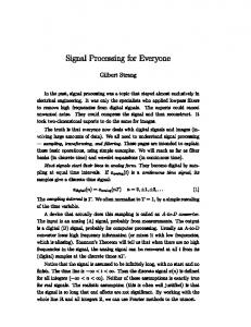
equation R ( t ) = t xˆ + t yˆ . We approximate the sensor peak as the reciprocal of the distance to the point of closest approach from a given platform to the target trajectory. Platforms are triggered, i.e., considered in the calculation, if the peak processing its data. meets or exceeds a threshold of 1. The trajectory of the target is shown as a curved line. The platforms that were triggered are shown as triangles, and the platforms that were triggered and used to calculate the local parameters are shown by diamonds. As shown in the figure, the algorithm does a good job of finding platforms to evenly cover the trajectory and avoid unnecessary transmissions from platforms that were not near the target trajectory. The average number of platforms in each of the groups that estimate local parameters at a point in the target trajectory is 7. This varied from 3 to 10. Care must be take to make the neighborhoods small enough so that there is adequate coverage of the trajectory, but large enough so that they contain an adequate number of platforms to determine local parameters. The extent to which this can be achieved will depend on platform density. The velocity errors for this experiment are shown in Figure 7. It shows the fraction error in speed,

result is that the platforms self organize into clusters spaced and timed along the target trajectory. The platform closest to the track within each cluster processes its data. IV.

2

VERIFICATION

This section provides some initial numerical experiments in testing the algorithms for platform clustering and velocity determination. Results from a numerical experiment, for platform clustering, which did not involve field data, are shown in figure 6. The platforms were deployed in a pseudo-random pattern, approximating what would result in a vehicle systematically covering an area and throwing out or dropping platforms randomly over a small area around the vehicle’s position. centers track triggered

15

untriggered

10

θ err

little bias. The average fractional error in speed is 0.1% and the average error in direction is –0.006 radians (-3.4 degrees). The estimates are also fairly accurate. The speed is accurate to within 10% and the direction within 60 for 80% of the measurements. The simulated experiments do not include sensor noise, however.

0 -10

-5

sest − strue , and the error in direction, strue ≡ θ est − θ true , in radians. These estimates show very

serr ≡

5

0

5

10

Figure 6. Platforms Used in Determining Local Parameters

V. CONCLUSIONS

The results are for a numerical experiment with a density of 1 platform per unit area and a neighborhood of 1 unit time and 4 units of length in both the x and y dimensions. The target position was defined by the

We have derived algorithms for target identification, called Semantic Information Fusion, which can combine semantic data, in the form of target attributes, with time-series data from platform sensors. This method is innovative because

Velocity Errors 0.400 0.300 0.200 0.100 0.000 -3.04 -0.100

-2.92

-2.56

-2.22

-1.34

-0.84

-0.32

0.50

1.29

1.96

-0.200 -0.300 time

Figure 7. Velocity Errors

fractional speed error direction error (rad)

2.49

2.79

it can compress time series data from heterogeneous sensors into semantic attributes. Dense sensor networks over large areas contain massive amounts of computing power in total but may be restricted in bandwidth and power consumption. Forming dynamic clusters around events of interest allows for processing multiple events in parallel over a geographic area. We have shown how dense networks can coordinate platforms around tracks and provide relevant processing with a minimum of bandwidth and power consumption related to inter-platform communications. This procedure is scalable and takes full advantage of the parallelism in the network. In addition, our method allows seamless integration of fixed and mobile, heterogeneous platforms. VI. A CKNOWLEDGEMENTS This effort is sponsored by the Defense Advance Research Projects Agency (DARPA) and the Space and Naval Warfare Systems Center, San Diego (SSC-SD), under grant number N66001-00-C-8947 (Semantic Information Fusion in Scalable, Fixed and Mobile Node Wireless Networks). The U.S. Government is authorized to reproduce and distribute reprints for Governmental purposes notwithstanding any copyright annotation thereon. The views and conclusions contained herein are those of the author’s and should not be interpreted as necessarily represent the official policies or endorsements, either expressed or imp lied, of the Defense Advanced Research Projects Agency (DARPA), the Space and Naval Warfare Systems Center, or the U.S. Government. VII. REFERENCES [1] [2]

[3] [4] [5]

[6]

[7]

[8]

[9]

S. S. Iyengar, R. L. Kashyap, and R. N. Madan, eds., IEEE Transactions on Systems, Man and Cybernetics, Special Issue on Distributed Sensor Networks, vol. 21, no. 5, 1991. Picinbono, B., and Boyer, M.P., “A new approach of decentralized detection,” International Conference on Acoustics, Speech, and Signal Processing, 1991. ICASSP -91, 1991, Page(s): 1329 -1332 vol.2. Tenney, R.R., and Sandell, N.R., “Detection with Distributed Sensors,” IEEE Trans. On Aerospace and Elec. Systems, Vol AES17, pp. 501-510: 1981. Jolliffe, I.T., Principal Component Analysis, New York : SpringerVerlag, c1986. Bhatnagar, V., Shaw, A., and Williams, R., "Improved Automatic Target Recognition Using Singular Value Decomposition," International Conference on Acoustics, Speech, and Singal Processing, 1998, Seattle, WA. Scott C. Deerwester, Susan T. Dumais, Thomas K. Landauer, George W. Furnas, Richard A. Harshman: “Indexing by Latent Semantic Analysis,” Journal of the American Society for Information Science (JASIS) Volume 41, Number 6, September 1990 391-407 Landauer T.K., Dumais S.T., “A solution to Plato’s problem: The Latent Semantic Analysis theory of Acquisition, Induction and Representation of Knowledge,” Pyschological Review, 104, 211-240, 1997. Goodwin, M. and Vetterli, M., “Atomic signal models based on recursive filter banks,” In Conference Record of the Thirty-First Asilomar Conf. on Signals, Systems, and Computers, November, 1997. Vaidyanathan, P.P., Multirate Systems and Filter Banks, Englewood Cliffs, NJ, Prentice-Hall, 1993.

[10] Signal Processing Toolbox for use with Matlab, The Mathworks, Inc., Natick, MA 1998. [11] Oppenheim, A.V., and Schaefer, R.W., Discrete-Time Signal Processing, Prentice Hall, Englewood Cliffs, NJ, 1989, pp 311-312. [12] Golub, G.H., and Van Loan, C.F., Matrix Computations, Johns Hopkins University Press, Baltimore, MA 1996. [13] Adelson, E.H. and Bergan J.R., “Spatiotemporal Energy Models for the Perception of Motion,” Journal of the Optical Society of America A, vol. 2, no. 2, pp. 284-299 (1985). [14] Adelson, E.H., Mechanisms for Motion Perception, Optics & Photonics News, August, pp. 24-30 (1991).