Department of Information Technologies. Joukahaisenkatu 3-5 B ... We study in this paper the semantics and proof rules for invariant-based pro- grams. The total ...
Ralph-Johan Back | Viorel Preoteasa
Semantics and Proof Rules of Invariant Based Programs
TUCS Technical Report No 903, June 2008
Semantics and Proof Rules of Invariant Based Programs Ralph-Johan Back Åbo Akademi University Department of Information Technologies Joukahaisenkatu 3-5 B, 20520 Turku, Finland
Viorel Preoteasa Åbo Akademi University Department of Information Technologies Joukahaisenkatu 3-5 B, 20520 Turku, Finland
TUCS Technical Report No 903, June 2008
Abstract Invariant based programming is an approach where we start to construct a program by first identifying the basic situations (pre- and postconditions as well as invariants) that could arise during the execution of the algorithm. These situations are identified before any code is written. After that, we identify the transitions between the situations, which will give us the flow of control in the program. The transitions are verified at the time when they are constructed. The correctness of the program is thus established as part of constructing the program. The program structure in invariant based programs is determined by the information content of the situations, using nested invariant diagrams. The control structure is secondary to the situation structure, and will usually not be well-structured in the classical sense, i.e., it is not necessarily built out of single-entry single-exit program constructs. The execution of an invariant diagram may start in any situation and will choose one of the enabled transitions in this situation, to continue to the next situation. In this way, the execution proceeds from situation to situation. Execution terminates when a situation is reached from which there are no enabled transitions. Because the execution could start and terminate in any situation, invariant-based programs can be thought of as multiple entry, multiple exit programs. The transitions may have statements with unbounded nondeterminism, because we allow specification statements in transitions. Invariant based programs are thus a considerable generalization of ordinary structured program statements, and defining their semantics and proof theory provides a challenge that usually does not arise for more traditional programming languages We study in this paper the semantics and proof rules for invariant-based programs. The total correctness of an invariant diagram is established by proving that each transition preserves the invariants and decreases a global variant. The proof rules for invariant-based programs are shown to be correct and complete with respect to an operational semantics. The proof of correctness and completeness introduces the weakest precondition semantics for invariant diagrams, and uses a special construction, based on well-ordered sets, of the least fixpoint of a monotonic function on a complete lattice. The results presented in this paper have been mechanically verified in the PVS theorem prover.
TUCS Laboratory Software Construction Laboratory
1 Introduction Invariant based programming is an approach where we start to construct a program by first identifying the basic situations (pre- and postconditions as well as invariants) that could arise during the execution of the algorithm. These situations are identified before any code is written. After that, we identify the transitions between the situations, which will give us the flow of control in the program. The transitions are verified at the time when they are constructed. The correctness of the program is thus established as part of constructing the program. The program structure in invariant based programs is determined by the information content of the situations, using nested invariant diagrams. The control structure is secondary to the situation structure, and will usually not be well-structured in the classical sense, i.e., it is not necessarily built out of single- entry single-exit program constructs. We refer to a program constructed in this manner as an invariant based program. The execution of an invariant based program may start in any situation and will choose one of the enabled transitions in this situation, to continue to the next situation. In this way, the execution proceeds from situation to situation. Execution terminates when a situation is reached from which there are no enabled transitions. Because the execution could start and terminate in any situation, invariant-based programs can be thought of as multiple entry, multiple exit programs. Termination of a program may also happen anywhere, not just at some prespecified exit points. The transitions may have statements with unbounded nondeterminism, because we allow specification statements in transitions. Invariant based programs are thus a considerable generalization of ordinary structured program statements, and defining their semantics and proof theory provides a challenge that usually does not arise for more traditional programming languages We study here the semantics and proof theory of invariant based programs [3, 4, 5]. The idea of invariant based programming is not new, similar ideas were proposed in the 70’s by John Reynolds [16], Martin van Emden [18], and RalphJohan Back [3, 4], in different forms and variations. Dijkstra’s later work on program construction also points in this direction [9], where he emphasizes the formulation of a loop invariant as a central step in deriving the program code. However, Dijkstra insists on building the program in terms of well-structured (single-entry single-exit) control structures, whereas there are no restrictions on the control structure in invariant based programming. Basic for these approaches is that the loop invariants are formulated before the program code is written. Eric Hehner [10] was working along similar lines, but chose relations rather than predicates as the basic construct. Invariant based programs are intended to be correct by construction, so proof of correctness is part of the programming process. For that purpose, we need to define the semantics of invariant based programs, give proof rules for showing that the program is correct, and we need to show that these proof rules are sound 1
(and preferably complete). But we cannot use existing theories directly, as they are typically based on well-structured control constructs. Our purpose here is therefore to define the semantics and proof theory of invariant based programs from scratch, and to show that the proof rules we give are both sound and complete with respect to the semantics we give for invariant based programs. We will proceed in the following way. We first describe invariant based programs in an intuitive way, to give a feel for the basic ideas behind this approach, and for the constraints and generalizations inherent in this approach. We begin the theoretical study of invariant based programs by defining their operational semantics. We will in fact define two different operational semantics. The first one is a small-step operational semantics that describes the way in which an invariant based program is executed by a computer. In essence, the small step semantics describes an interpreter for the programming language. The second one is a big step operational semantics that describes the overall behavior of an invariant based program, essentially as a mapping from input states to possible output states. This semantics is only concerned with the input output behavior of the program. It allows us to define basic properties of program execution, like partial correctness and termination. We show that the small step semantics and the big step semantics are equivalent. In other words, any correctness property that holds for the big step semantics of an invariant based program will also hold for the small step execution of the program, and vice versa. We then define a weakest precondition semantics for invariant based programs. The weakest precondition semantics is compositional, and allows us to directly compute the basic correctness properties of an invariant based program. We show that the weakest precondition semantics is equivalent to the big step operational semantics. The weakest precondition semantics does not, however, give us a practical method for proving program correctness, because it uses least fixpoints to determine the semantics of loops. We get around this obstacle by giving a collection of Hoare-like [11] total correctness proof rules for invariant based program. We show that the proof rules are sound with respect to the weakest precondition semantics. This means that if we prove, using these proof rules, that our invariant based program is correct, then it will also be correct according to the weakest precondition semantics. Because we have shown that the weakest precondition semantics is equivalent to the big step semantics, which in turn is equivalent to the small step semantics, we get the following basic property: If we have proved that an invariant based program is correct using the given proof rules, then any execution of the invariant based program that respects the small step semantics will be correct. This means that our proof system is sound. We also study the converse problem: Assume that we have a correct invariant based program that is executed according to the small step semantics. Can we then prove that the program is correct using the given proof rules for invariant 2
based programs? The answer to this question is positive, i.e., our proof system is also complete. In the end, this means that our proof system is both sound and complete for invariant based programs. The theory of invariant based programs has been completely mechanized in the PVS interactive proof system [15]. This gives a very solid foundation for our results. This PVS formalization depends on the well-ordering theorem which says that any set can be well-ordered. Both the soundness and completeness results we have for invariant based programs are consequences of more general results for monotonic functions on a complete lattice. We give a special construction, based on a well ordered set, of the least fixpoint of a monotonic function on a complete lattice. The completeness theorem is a consequence of this construction. We allow specification statements in our programs, so our semantics may have unbounded nondeterminism. This means that we need to go beyond natural numbers and use well ordered relations [13] or ordinals [1] when proving completeness. This is due to the fact that unbounded non-deterministic statements are not continuous. Nipkow [13] presents an Isabelle [14] formalization of complete Hoare proof rules for recursive parameterless procedures in the context of unbounded nondeterminism. Our programming language is, however, more general than the one studied in [13], because it features multiple-entry, multiple-exit statements, and a more general recursion mechanism. Our proof of completeness is also more general and simpler than the one in [13], and we believe that it could be applied unmodified to richer programming constructs, such as procedures with parameters and local variables. The framework that we build allows us to study termination proofs for invariant based programs in more detail, and to justify specific proof rules for termination. Proving termination of invariant based programs is more difficult than usually, because the control structure is unconstrained. This means that our loops need not be nested, we can have intersecting loops, loops with exits in the middle (multiple exit loops) and loops that can be entered in the middle (multiple entry loops). Nevertheless, the framework that we have built allows us to formulate new proof techniques for termination, that are more general than existing ones, but which we still can prove to be sound.
2 Syntax of invariant diagrams Let State be an unspecified type of states and Var be the type of all program variables. For x ∈ Var, the type of the variables x, denoted T.x, contains all values that can be assigned to x. Intuitively a state s from State gives the values to the program variables. Formally, we access and update program variables using two functions. val.x : State → T.x and set.x : T.x → State → State. For x ∈ Var, s ∈ State, and a ∈ T.x, valx.s is the value of x in state s, and setx.a.s is the 3
state obtained from s by setting the value of location x to a. The behavior of these functions is described using a set of axioms [6]. For the purpose of this paper we do not need to consider in greater details the treatment of program variables. Let Bool be the set of Boolean values. Predicates, denoted Pred, are the functions from State → Bool. Relations, denoted by Rel, are functions from State to Pred. We denote by ⊆, ∪, and ∩ the predicate inclusion, union, and intersection respectively. The type Pred together with inclusion forms a complete Boolean algebra. We use higher-order logic [7] as the underlying logic. If f : A → B is a function and x ∈ A, then the function application is denoted by f.x (f dot x). An invariant diagram is a directed graph where nodes are labeled with invariants (predicates) and edges are labeled with transitions (program statements). The transitions are non-iterative programs built from assertions, assumptions, demonic updates, demonic choices, and sequential compositions. The abstract syntax of transitions is defined by the following recursive data type: Trs = Assert(Pred) | Assume(Pred) | Update(Rel) | Choice(Trs, Trs) | Comp(Trs, Trs) If p is a predicate, R is a relation, and S, T are transitions, then we use the notations {p}, [p], [R], S ⊓ T, S ; T for the constructs Assert, Assume, Update, Choice, and Comp, respectively. Intuitively the execution of the assert statement {p} and the assume statement [p] starting in a state s in which p is true behave as skip. If p is false in s, then {p} fails and [p] is not enabled. The demonic update [R], when starting in a state s, terminates in a nondeterministically chosen state s′ such that R.s.s′ . If there is no state s′ such that R.s.s′ , then [R] is not enabled. The execution of the demonic choice S ⊓ T nondeterministically chooses S or T . The transition S ; T is the sequential composition of the transitions S and T . We model both assignments and nondeterministic assignments using the demonic update: (x := e)
= [λs, s′ • s′ = set.x.(e.s).s]
[x := a • b.a] = [λs, s′ • (∃a • s′ = set.x.a.s ∧ b.a.s)] A transition S is enabled, when starting from a state s, if it is possible to avoid any assume or demonic choice statements which are not enabled. For example the transition S = ([x < 4]; x := x + 1; [x > 1]) ⊓ ([x > 10]; x := 3) is enabled for all states where x is 1, 2, 3 or greater than 10. If x is 1 in the initial state s, then we chose the first part of the choice in S, and all assume statements in this part are enabled. The guard of a transition S is a predicate which is true for all states from which S is enabled. We will define formally later the notions enabled 4
and guard, but we have introduced them here informally to explain the intuition behind invariant based programs. Let I be a nonempty set of indexes. Formally an invariant diagram ID is a tuple (P, D) where P : I → Pred are the invariants and D : I × I → Trs are the transitions. D is called a transition diagram and the elements of I are called situations. The invariant diagrams are represented as special graphs. The nodes are represented by rectangles. Inside the rectangles we write the invariants. The transitions are represented by directed edges in the graph, labeled with the transition statements. Figure 1 represents an invariant diagram. The program represented in this figure searches if an element is member in an array of numbers. 1
n, x ∈ nat ∧ a : {0, 1, . . . , n − 1} → nat 2
0 ≤ i ≤ n ∧ (∀j • 0 ≤ j < i ⇒ a.j 6= x) 3
4
i=n
i < n ∧ a.i = x
(1) [i = n]
[i < n ∧ a.i = x]
i := 0 [i < n ∧ a.i 6= x]; i := i + 1
In Figure 1 the situations are 1, 2, 3, 4. In practice, it is very often the case that the invariant of a situation i is stronger than the invariant of another situation j (Pi = Pj ∧ q). In this case we draw the situation i inside situation j, and we label i only with the predicate q. The invariant of situation i is the conjunction of q and the labels of all situations containing the situation i. For example in (1), the invariant of situation 4 is the conjunction of the predicate labels of situations 1, 2, and 4: (n, x ∈ nat ∧ a : {0, 1, . . . , n − 1} → nat) ∧(0 ≤ i ≤ n ∧ (∀j • 0 ≤ j < i ⇒ a.j 6= x)) ∧(i < n ∧ a.i = x) Intuitively the execution of an invariant diagram starts from an initial situation and follows the transitions which are enabled. At each step the invariant of the current situation must be satisfied by the current value of the program variables. The execution terminates in a situation i when i is reached, and there are no enabled transitions from i. 5
The formal definition of an invariant diagram requires that there must be a transition between any two situations. However in our example (1) this requirement is not meet, there is no transition between situation 3 and 4. Formally, when there is no transition between two situations, we assume that there is a default transition (miracle = [false]) which is always disabled. Always, when we draw the diagram, we omit the transitions labeled by miracle. Invariant programs are more general than imperative programs, they can be thought of as multiple entry, multiple exist programs. In principle an invariant program could start and terminate in any situation. If the program represented in (1) starts in situation 1, then it can terminate in situations 2 if the element x is not member of the array a or in situation 3 otherwise.
3 Operational semantics We introduce in this section smallstep and bigstep operational semantics for invariant diagrams and we prove their equivalence.
3.1 Small step semantics We introduce first the smallstep semantics for transitions. If S, T ∈ Trs and s, s′ ∈ Σ , then the smallstep relation (s, S) → (s′ , T ) is true if from state s we get to s′ by executing one step (atomic statement) of S, and T is the transition S from which the executed step is removed. If the transition S consists of only one step, then the smallstep relation becomes (s, S) → (s′ , []). We denote by (s, S) → ⊥ the fact that the execution of S fails in the next step when starting from s. b.s (s, {b}) → (s, [])
¬b.s (s, {b}) → ⊥
b.s (s, [b]) → (s, [])
R.s.s′ (s, [R]) → (s′ , [])
(s, S ⊓ T ) → (s, S)
(s, S ⊓ T ) → (s, T )
(s, S) → (s′ , S ′ ) (s, S ; T ) → (s′ , S ′ ; T )
(s, S) → (s′ , []) (s, S ; T ) → (s′ , T )
(s, S) → ⊥ (s, S ; T ) → ⊥
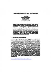
Let D be a transition diagram. Figure (2) represents one transition of D labeled by S ′ ; S. We assume that the execution reached the state s in this transition. Then the tuple (s, S, i, D) denotes the status of the execution. The execution is in state s, and it proceeds towards the situation i by executing S. If the execution reaches i in a state s′ , then status of the execution is denoted by (s′ , [], i, D). j
S′
s
6
S
i
(2)
The smallstep relation (s, A, i, D) → (s′ , B, i, D), where A, B ∈ Trs ∪ {[]}, is defined by the following rules. (s, Di,j ) → (s′ , S) (s, S) → (s′ , S ′ ) (s, [], i, D) → (s′ , S, j, D) (s, S, i, D) → (s′ , S ′ , i, D) The transition diagram could fail in (s, A, i, D), denoted by (s, S, i, D) → ⊥, if some available transition could fail in next step. (s, Dij ) → ⊥ (s, [], i, D) → ⊥
(s, S) → ⊥ (s, S, i, D) → ⊥
3.2 Big step semantics Similarly to smallstep semantics, we introduce first the bigstep semantics of transitions. If S ∈ Trs and s, s′ ∈ Σ, then the bigstep relation (s, S) s′ is true if there is an execution of S starting in s and ending in s′ . (s, S) s′ is defined by induction on the structure of S. b.s (s, {b})
s
(s, S) s′ (s, S ⊓ T ) s′
b.s (s, [b])
R.s.s′ (s, [R]) s′
s
(s, T ) s′ (s, S ⊓ T ) s′
(s, S) s′ ∧ (s′ , T ) (s, S ; T ) s′′
s′′
A transition S, starting from a state s, may fail (denoted (s, S) ⊥) if some of its executions leads to a false assertion.Failure is defined by induction on the structure of S. ¬b.s (s, {b})
⊥
(s, S) ⊥ (s, S ; T ) ⊥
(s, S) ⊥ (s, S ⊓ T ) ⊥ (s, S) s′ ∧ (s′ , T ) (s, S ; T ) ⊥
(s, T ) ⊥ (s, S ⊓ T ) ⊥ ⊥
Similarly, the execution of S, starting from a state s, is miraculous or disabled (denoted (s, S) ⊤) if any of its executions leads to a false assumption or to a demonic update [R] which cannot progress. The demonic update [R] cannot progress from a state s if for all states s′ , R.s.s′ is false. ¬b.s (s, [b]) ⊤ (s, S) ⊤ (s, S ; T ) ⊤
∀s′ • ¬R.s.s′ (s, [R]) ⊤ (s, S) 6
(s, S) ⊤ ∧ (s, T ) (s, S ⊓ T ) ⊤
⊥ ∧ (∀s′ • (s, S) (s, S ; T ) 7
s′ ⇒ (s′ , T ) ⊤
⊤
⊤
Theorem 1 Miracle could be defined in terms of bigstep and fail. (s, S)
⊥ ∧ (∀s′ • (s, S) 6
⊤ ⇔ ((s, S) 6
s′ ))
If D ∈ I × I → Trs, s, s′ ∈ Σ, and i, j ∈ I, then the bigstep relation (s, i, D) (s′ , j) is true if there is an execution from state s and situation i, following the enabled transitions D, ending in state s′ and situation j, and all transitions from state s′ and situation j are disabled. The execution of D from state s and situation i may fail, denoted (s, i, D) ⊥, if there is a situation j such that the transition Di,j may fail when starting from s. (s, Di,j )
s′ ∧ (s′ , j, D) (s′′ , k) (s, i, D) (s′′ , k)
(∀j • (s, Di,j ) ⊤) (s, i, D) (s, i)
(s, Di,j ) (s, i, D)
⊥ ⊥
When starting from state s and situation i, the transition diagram T terminates, denoted (s, i, T ) ↓, if all execution paths starting in s, i are finite and do not fail. (∀j • (s, Di,j ) ⊤) (s, i, D) ↓ (s, i, D) 6
⊥ ∧ (∀j, s′ • (s, Di,j ) (s, i, D) ↓
s′ ⇒ (s′ , j, D) ↓)
The bigstep semantics is useful in establishing further properties of transition diagrams, however it does not give a very intuitive understanding of how invariant diagrams are executed. In the next section we introduce the smallstep operational semantics for transition diagrams which is closer to the way the diagrams would be executed by a computer.
3.3 Connection between bigstep semantics and smallstep semantics. The small step semantics is equivalent to the bis step semantics in the following sense. If the execution of D starts from a state s and a situation i and proceeds in small steps until a state s′ in situation j, and there are no transitions enabled from (s′ , j), then this is equivalent with D performing a big step from (s, i) to (s′ , j). ∗ In the next theorems the symbol → denotes the reflexive and transitive closure of the relation →. ∗
Theorem 2 (s, S)
s′ ⇔ (s, S) → (s′ , [])
Theorem 3 (s, S)
⊥ ⇔ (s, S) → ⊥
∗
8
We define the miracle in the smallstep semantics by ∗ ∗ (s, S) 99K ⊤ = ¬(s, S) → ⊥ ∧ (∀s′ • ¬(s, S) → (s′ , [])) Theorem 4 (s, i, D)
∗
(s′ , j) ⇔ (s, [], i, D) → (s′ , [], j, D) ∧ (∀k • (s′ , Dj,k ) 99K ⊤)
In the remainder of this paper we will work with bigstep semantics only.
4 Weakest precondition and predicate transformers Proving correctness of invariant diagrams is unfeasible using the operational semantics. We will therefore define here a compositional semantics for invariant based programs, based on the notion of weakest preconditions.
4.1 Weakest precondition and predicate transformers for transitions. If p, q ∈ Pred , and S ∈ Trs then the Hoare total correctness triple p {| S |} q denotes the fact that if the transition S start in state s from p, then it terminates in a state from q. The Hoare triple p {| S |} q is valid, denoted |= p {| S |} q, if
⊥ ∧ (∀s′ • (s, S)
|= p {| S |} q ⇔ (∀s • p.s ⇒ (s, S) 6
s′ ⇒ q.s′ ))
(3)
The weakest precondition for a transition S and a post condition q is a predicate, wp.S.q ∈ Pred. For a state s, wp.S.q.s is true if the execution of S does not fail and always terminates in a state s′ from q (q.s′ is true). Using the bigstep operational semantics for transitions we define the weakest precondition by: wp.S.q.s = (s, S) 6
⊥ ∧ (∀s′ • (s, S)
s′ ⇒ q.s′ ).
The validity of Hoare triples could be expressed equivalently using the weakest precondition: |= p {| S |} q ⇔ p ⊆ wp.S.q
(4)
Relation (4) reduces the proof of validity of a Hoare triple to an inclusion of predicates. However the predicate wp.S.q is defined in terms of bigstep semantics, and the proof of the statement p ⊆ wp.S.q is still unfeasible in practice. For S ∈ Trs we define, by induction on S, the predicate transformer associated to S, pt.S : Pred → Pred by: 9
pt.{p}.q
= p∧q
pt.[p].q
= ¬p ∨ q
pt.[R].q.s
= (∀s′ • R.s.s′ ⇒ q.s′ )
pt.(S ⊓ T ).q = pt.S.q ∧ pt.T.q pt.(S ; T ).q
= pt.S.(pt.T.q)
Theorem 5 For all S ∈ Trs wp.S = pt.S Proof. By induction on the structure of S. Using Theorem 5 and relation (4) it follows
�
|= p {| S |} q ⇔ p ⊆ pt.S.q
(5)
The relation (5) reduces the proof of the validity of a Hoare triple to an inclusion of predicates. These predicates are defined in terms of the predicates p, q, the predicates and expressions occurring in S using Boolean connectives (∧, ∨, → , . . .). Theorem 6 For all S ∈ Trs the predicate transformer pt.S is monotonic. Proof. This fact follows directly from Theorem 5 and the definition of wp.S. � The guard of a transition S is a predicate denoted grd.S ∈ Pred and is true for all states s from which the execution of S is enabled. grd.S = ¬pt.S.false Theorem 7 The guard of a transition S is true in a state s if and only if the execution of S starting from s is not miraculous: grd.S.s ⇔ (s, S) 6
⊤
Proof. Using Theorem 1, Theorem 5, and the definitions of grd and wp. grd.S.s =
{Definition of grd} ¬pt.S.false
=
{Theorem 5} 10
¬wp.S.false =
{Definition of wp} ¬((s, S) 6
=
⊥ ∧ (∀s′ • (s, S)
{Boolean properties} ¬((s, S) 6
=
s′ ⇒ false.s′ ))
⊥ ∧ (∀s′ • (s, S) 6
s′ ))
{Theorem 1} (s, S) 6
⊤
�
4.2 Weakest precondition and predicate transformers for transition diagrams The Hoare triples for diagrams have similar interpretations to those of the transitions. However, a diagram may be executed starting in any situation and it may terminate in any situation. Let P, Q : I → Pred and D : I × I → Pred. The diagram Hoare total correctness triple, P {| D |} Q, is true if whenever the execution of D starts in a state s from a situation i, such that P.i.s is true, then D always terminates, and if D terminates in a state s′ and a situation j, then Q.j.s′ is true. The predicate P.i is the precondition of D when starting from situation i. Similarly, Q.j is the postcondition of D when terminating in situation j. The Hoare triple P {| D |} Q is valid, denoted |= P {| D |} Q, if |= P {| D |} Q ⇔
(6) (∀i, s • P.i.s ⇒ (s, i, D) ↓ ∧(∀j, s′ • (s, i, D)
(s′ , j) ⇒ Q.j.s′ ))
The weakest precondition for a diagram D and a postcondition Q is an indexed predicate wp.D.Q : I → Pred. For a state s and a situation i, wp.D.Q.i.s is true if the execution of D from s, i always terminates, and if it terminates in a state s′ and a situation j then Q.j.s′ is true. Using the bigstep operational semantics for diagrams we define the weakest precondition by: wp.D.Q.i.s = (s, i, D) ↓ ∧(∀j, s′ • (s, i, D)
(s′ , j) ⇒ Q.j.s′ ).
The validity of diagram Hoare triples could be expressed equivalently using the weakest precondition: |= P {| D |} Q ⇔ P ⊆ wp.D.Q 11
(7)
Relation (7) reduces the proof of validity of a Hoare triple to an inclusion of indexed predicates. However, similarly to transitions’ case, proving P ⊆ wp.D.Q is unfeasible in practice due to the bigstep semantics expressions occurring in wp. The guard of a situation i in a diagram D is a predicate grd.D.i ∈ Pred which is true in those states in which the execution from situation i is enabled: grd.D.i =
_
grd.Di,j
j∈I
Let Dpt = (I → Pred) → (I → Pred). For D ∈ I × I → Trs let F.D : Dpt → Dpt be the monotonic function given by
F.D.U.Q.i.s = (∀j • pt.Di,j .(U.Q.j).s) ∧ (¬grd.D.i.s ⇒ Q.i.s) The predicate transformer associated to D, pt.D : Dpt, is the least fix point of F : pt.D = µ F.D Theorem 8 wp.D = pt.D Proof. We prove that wp.D is fixpoint for F.D and it is smaller than any other fixpoint. � Using Theorem 8 and relation (7) it follows |= P {| D |} Q ⇔ P ⊆ pt.D.Q
(8)
The relation (8) reduces the proof of the validity of a Hoare triple to an inclusion of predicates. However, unlike for transitions, the predicate pt.D.Q is a least fixpoint expression, and proving P ⊆ pt.D.Q is unfeasible in practice. Theorem 9 For all D ∈ I × I → Trs the predicate transformer pt.D is monotonic. Proof. This fact follows directly from Theorem 8 and the definition of wp.D. �
5 Axiomatic semantics The weakest precondition semantics does not allow us to prove correctness of programs in practice, because of the use of the least fixed point operator. We need to define Hoare like proof rules for invariant based programs to establish correctness in practice. 12
5.1 Hoare rules for transitions The Hoare triple p {| S |} q is correct, denoted ⊢ p {| S |} q, if it can be proved using following Hoare rules. ∀s • p.s ⇒ r.s ∧ q.s ⊢ p {| {r} |} q
∀s • p.s ∧ r.s ⇒ q.s ⊢ p {| [r] |} q
∀s, s′ • p.s ∧ R.s.s′ ⇒ q.s′ ⊢ p {| [R] |} q
⊢ p {| S |} q ⊢ p {| T |} q ⊢ p {| S ⊓ T |} q
⊢ p {| S |} r ⊢ r {| T |} q ⊢ p {| S ; T |} q
⊢ p {| S |} q p′ ⊆ p ∧ q ⊆ q ′ ⊢ p′ {| S |} q ′
The validity is equivalent to proving correctness using the Hoare rules, and, in practice, the Hoare rules are used to prove the correctness of transitions. Theorem 10 (Correctness) ⊢ p {| S |} q ⇒ |= p {| S |} q Proof. By induction on the structure of S.
�
Theorem 11 wp.S.q {| S |} q. Proof. We prove pt.S.q {| S |} q by induction on the structure of S.
�
Theorem 12 (Completeness) |= p {| S |} q ⇒ ⊢ p {| S |} q. Proof. By the definition of |= p {| S |} q and wp.q it follows p ⊆ wp.q and by theorem 11 and Hoare consequence rule it follows p {| S |} q. � Before introducing the proof rules for diagrams we need some definitions and properties of complete lattices and fixpoints.
5.2 Complete lattices and fixpoints This section introduces some results about fixpoints in complete lattices [8]. These results are the main tools in proving correctness and completeness of the proof rules for invariant diagrams. A partially ordered (poset) set hL, ≤i is a complete lattice if every subset of L has least upper bound or equivalently greatest lower bound. For a subset A of 13
L, ∨A ∈ L denotes the least upper bound (join) of A and ∧A ∈ L denotes the greatest lower bound (meet) of A. If L is a complete lattice, than the least (bottom) and the greatest (top) elements of L exist and they are denoted by ⊥, ⊤ ∈ L, respectively. If A is a nonempty set and L is a lattice, than the pointwise extension of the order on L to A → L is also a complete lattice. The operations meet, join, bottom, and top on A → L are also the pointwise extensions of the corresponding operations on L. If hA, ≤i is a partially ordered set, then the set of monotonic m functions from A to L, denoted A → L is also a complete lattice. The order, meet, m join, top, and bottom on A → L are the pointwise extensions of the corresponding operations on L. For a complete lattice L, MF.L is the complete lattice of monotonic functions from L to L. The Boolean algebra with two elements Bool, the predicates Pred, the indexed predicates I → Pred, and the monotonic predicate transformers are complete lattices. We list briefly some properties of well founded and well ordered sets that are needed in this paper. For a comprehensive treatment of this subject see [12]. A partially ordered set hW,