Semantics-guided Clustering of Heterogeneous XML Schemas Pasquale De Meo1 , Giovanni Quattrone1 , Giorgio Terracina2 , and Domenico Ursino1 1
DIMET, Universit` a Mediterranea di Reggio Calabria, Via Graziella, Localit` a Feo di Vito, 89060 Reggio Calabria, Italy, 2 Dipartimento di Matematica, Universit` a della Calabria, Via Pietro Bucci, 87036 Rende (CS), Italy
[email protected],
[email protected],
[email protected],
[email protected]
Abstract. In this paper we illustrate an approach for clustering semantically heterogeneous XML Schemas. The proposed approach is driven by the semantics of the involved Schemas that is defined by means of the interschema properties existing among concepts represented therein; interschema properties taken into account by our approach are synonymies (indicating that two concepts have the same meaning), hyponymies (denoting that a concept has a more specific meaning than another one), and overlappings (indicating that two concepts are neither synonyms nor one hyponym of the other, but represent, to some extent, the same reality). An important feature of our approach consists of its capability of being integrated with almost all the clustering algorithms already proposed in the literature. Both a theoretical and an experimental analysis on the complexity of our approach are presented in the paper. They show that our approach is scalable and particularly suited in application contexts characterized by a great number and a large variety of XML Schemas.
1
Introduction
Clustering is the process of grouping a set of physical or abstract objects into classes of similar objects, called clusters [1], in such a way that those objects belonging to the same cluster are as similar as possible, whereas those ones belonging to different clusters are as dissimilar as possible. Clustering has its roots in many areas, including Data Mining, Statistics, Biology and Machine Learning. Its applications are extremely various and range from Economy to Finance, from Biology to Sociology, and so on. Clustering can play a key role also in the Web; in fact, in this scenario, numerous applications that largely benefit of clustering have been proposed [2,3]. In the Web context, a specific activity in which clustering can play a key role consists of grouping semantically heterogeneous information sources. In fact, currently, both the number and the semantic heterogeneity of information sources S. Spaccapietra et al. (Eds.): Journal on Data Semantics IX, LNCS 4601, pp. 39–81, 2007. c Springer-Verlag Berlin Heidelberg 2007
40
P. De Meo et al.
available on the Web are strongly increasing. As a consequence, it appears extremely important the definition of approaches for clustering them into homogeneous classes. On the contrary, as for data representation format and data exchange, the World Wide Web Consortium foretells a certain uniformity for the future and, to this purpose, proposes the usage of the XML language. The growing importance of both clustering and XML stimulated, in the past, various researchers to study clustering techniques for XML sources [4,5,6,7]. Many of these techniques were “structural”, i.e., they aimed at defining groups of structurally similar XML sources [4,6]. Clearly, the structural similarity (resp., dissimilarity) of two information sources is an indicator of their semantic similarity (resp., dissimilarity); however, often, it could be not sufficient [8,9,10]. As an example, consider a list of orders (i.e., a list of products bought by a customer in a commercial transaction); in an XML Schema this list could be represented in very different ways. In a first representation we could have an element, order, containing two sub-elements, product and customer; in a second representation we could have three elements, product, customer and order, at the same level, and we could implement their relationships by means of key/keyref constructs. Clearly, these two representations would lead to documents extremely different from a structural point of view; nonetheless, these documents might be extremely similar from a semantic standpoint. In the literature various methods for defining information source semantics have been proposed; one of the most commonly adopted methods is based on the exploitation of the so-called interschema properties, [11,8,10,12], i.e., terminological and structural relationships existing among concepts belonging to different information sources. The most important interschema properties are synonymies (indicating that two concepts have the same meaning), homonymies (denoting that two concepts have different meanings, yet having the same name), hyponymies/hypernymies (indicating that a concept has a more specific meaning than another one) and overlappings (denoting that two concepts are neither synonyms nor one hyponym of the other, but represent, to some extent, the same reality). In order to better understand the importance of interschema properties, consider the following example. Let S1 be an XML Schema concerning vegetables and let S2 be an XML Schema about factories; assume that both S1 and S2 contain the element “plant”. If we consider only their name, we could erroneously conclude that the element “plant” of S1 and the element “plant” of S2 represent the same concept; on the contrary, if we consider their semantics, we could state that an interschema property (i.e., an homonymy) holds between these two elements and, consequently, that they represent different concepts. In the literature some approaches for clustering XML sources, taking into account their semantic similarities, have been proposed too [5,7]. However, in these approaches, source similarity is determined by considering only concept similarities that, in the context of interschema properties, correspond to synonymies. In our opinion they are extremely interesting; however, they could be
Semantics-guided Clustering of Heterogeneous XML Schemas
41
further refined if, in addition to synonymies, also other interschema properties, such as hyponymies and overlappings, would be considered. This paper aims at providing a contribution in this setting; in fact, it presents an approach for clustering semantically heterogeneous information sources; the proposed approach takes not only synonymies, but also hyponymies and overlappings, into account. In order to clarify the importance of hyponymies and overlappings in the clustering process, consider the following example. Let S1 be an XML Schema having an element house, described by four sub-elements, namely bedroom, bathroom, kitchen and garden. Let S2 be an XML Schema containing the element firstfloor, characterized by the sub-elements kitchen and lounge, and the element secondfloor, characterized by the sub-elements garden, bedroom, bathroom and garret. Now, neither firstfloor nor secondfloor would be recognized as synonymous with house and, consequently, the corresponding portions of schemas would be considered completely distinct by a clustering approach taking only synonymies into account. However, both firstfloor and secondfloor should be considered overlapping with house, since the information content of house is distributed over them. As a consequence, a clustering approach taking also overlappings into account would recognize that there is a form of similarity also in these portions of S1 and S2 and, hence, would compute more refined clusters. We point out that the present paper has not been conceived for defining a new clustering algorithm; on the contrary, it aims at allowing the application, to our reference context, of most of the existing clustering algorithms. As a matter of fact, in the literature, a great number of clustering algorithms, characterized by extremely various features, already exists, and other ones will be presumably proposed in the future. As a consequence, allowing the application of all these algorithms to our reference context would provide the user with the availability of a large variety of clustering tools, characterized by different peculiarities. The key for reaching such a result is the exploitation of the so called Dissimilarity Matrix [1]; this is, in fact, the data structure which almost all the clustering algorithms already proposed in the literature operate upon. The rows and the columns of this matrix represent the objects to cluster; its generic element M [i, j] denotes the distance, i.e., the dissimilarity, between the objects i and j. Generally, M [i, j] is a non-negative number that is as closer to 0 as i and j are similar. Our approach exploits interschema properties for finding the dissimilarity degree between two XML Schemas and, consequently, for constructing the Dissimilarity Matrix. Since some clustering algorithms require the involved objects to be represented as points in a metric space (see Section 3.5), in order to allow the applicability of the maximum possible number of clustering algorithms to our reference context, we define the dissimilarity among XML Schemas by exploiting a suitable euclidean space. The outline of the paper is as follows: Section 2 describes a technique for extracting interschema properties. Section 3 provides a detailed description of
42
P. De Meo et al.
the proposed approach. The experiments we have carried out for evaluating its performance are presented in Section 4. Some possible applications are described in Section 5. Related works are examined in Section 6. Finally, in Section 7, we draw our conclusions.
2
Preliminaries
As pointed out in the Introduction, the clustering approach we are presenting in this paper requires interschema properties concerning involved sources to be provided as input. These properties might be derived by applying any approach proposed in the literature for this purpose (see, for example, [8,13,14,15,10,12]). In order to illustrate the main features of an interschema property extraction task, in this section we describe an approach for deriving interschema properties; this approach has been already presented in detail in [16]. Interschema properties we are considering in this paper are synonymies, hyponymies/hyperonymies and overlappings. The interschema property extraction approach we are introducing in this section is specialized for XML, almost automatic, semantic, and takes the intensional component of the involved XML sources into account. It is based on the observation that, given two concepts belonging to different information sources, an interesting and powerful way for determining their semantics consists of examining their neighborhoods, since the concepts and the relationships which they are involved in contribute to define their meaning [12]. In addition, it exploits two further indicators for defining the semantics of involved data sources in a more precise fashion; these indicators are the types and the cardinalities of the elements and the attributes belonging to the XML Schemas into consideration. In XML Schemas, concepts are expressed by elements or attributes. Since, for the interschema property extraction task, it does not appear relevant to distinguish concepts represented by elements from concepts represented by attributes, we introduce the term x-component for denoting an element or an attribute in an XML Schema. In order to compute the neighborhood of an x-component, it is necessary to define a “Semantic Distance” between two x-components of the same schema; this distance considers how much the corresponding x-components are semantically related. To this purpose we introduce some boolean functions that allow the strength of the relationship existing between two x-components x ν and xµ of an XML Schema S to be determined. These functions are: – veryclose(xν , xµ ), that returns true if and only if: (i) xµ = xν , or (ii) xµ is an attribute of xν , or (iii) xµ is a simple sub-element of xν ; – close(xν , xµ ), that returns true if and only if: (i) xµ is a complex sub-element of xν , or (ii) xµ is an element of S and there exists a keyref constraint stating that an attribute of xν refers to a key attribute of xµ ; – near(xν , xµ ), that returns true if and only if either veryclose(xν , xµ ) = true or close(xν , xµ ) = true;
Semantics-guided Clustering of Heterogeneous XML Schemas
43
– reachable(xν , xµ ), that returns true if and only if there exists a sequence of distinct x-components x1 , x2 , . . . , xn such that: x1 = xν , near(x1 , x2 ) = near(x2 , x3 ) = . . . = near(xn−1 , xn ) = true, xn = xµ . The exploitation of the functions introduced above allows each pair hx ν , xµ i of an XML Schema to be associated with a coefficient called Connection Cost. It is a measure of the correlation degree existing between xν and xµ and indicates how much the concept expressed by xν is semantically close to the concept represented by xµ ; in other words, it represents the ability of the concept associated with xµ to characterize the concept associated with xν . More formally, the Connection Cost from xν to xµ , denoted by CC(xν , xµ ), is defined as: 0 if veryclose(xν , xµ ) = true 1 if close(xν , xµ ) = true CC(xν , xµ ) = Cνµ if reachable(xν , xµ ) = true and near(xν , xµ ) = f alse ∞ if reachable(xν , xµ ) = f alse Here Cνµ = minxα (CC(xν , xα ) + CC(xα , xµ )) for each xα such that reachable(xν , xα ) = reachable(xα , xµ ) = true. Finally, given a non-negative integer i, we define the ith neighborhood of an x-component xν of an XML Schema S as the set of x-components of S having a Connection Cost from xν lesser than or equal to i. More formally, the ith neighborhood of xν is defined as: nbh(xν , i) = {xµ | xµ is an x-component of S, CC(xν , xµ ) ≤ i} In order to verify if an interschema property holds between two x-components, our approach compares their neighborhoods, their cardinalities and their data types. In addition, it exploits a thesaurus storing lexical synonymies holding among the terms of a language; specifically, it uses the English language and WordNet [17]. If necessary, different (possibly already defined) domain-specific thesauruses might be exploited. Since neighborhood comparison plays a key role in the interschema property extraction task, we first introduce it and, then, illustrate the property extraction task in detail. 2.1
Neighborhood Comparison
Given two x-components xν and xµ , belonging to different XML Schemas, and two corresponding neighborhoods nbh(xν , v) and nbh(xµ , v), there could exist different relationships between them. Specifically, three possible relationships, namely similarity, comparability and generalization, could be taken into account. All of them are derived by computing suitable objective functions on the maximum weight matching associated with a bipartite graph obtained from the x-components of nbh(xν , v) and nbh(xµ , v). In the following we indicate by BG(xν , xµ , v) = hN Set(xν , xµ , v), ESet(xν , xµ , v)i the bipartite graph associated with nbh(xν , v) and nbh(xµ , v); when it
44
P. De Meo et al.
is not confusing, we shall use the notation BG(v) instead of BG(xν , xµ , v). In BG(v), N Set(v) = P Set(v) ∪ QSet(v) represents the set of nodes; there is a node in P Set(v) (resp., QSet(v)) for each x-component of nbh(xν , v) (resp., nbh(xµ , v)). ESet(v) is the set of edges; there is an edge between p ∈ P Set(v) and q ∈ QSet(v) if: (i) a lexical synonymy between the names of the x-components xp and xq , associated with p and q, is stored in the reference thesaurus; (ii) the cardinalities of xp and xq are compatible; (iii) their data types are compatible (this last condition must be verified only if xp and xq are attributes or simple elements). Here, the cardinalities of two x-components are considered compatible if the intersection of the intervals defined by them is not empty. Compatibility rules associated with data types are analogous to the corresponding ones valid for high level programming languages. The maximum weight matching for BG(v) is the set ESet0 (v) ⊆ ESet(v) of edges such that, for each node x ∈ P Set(v) ∪ QSet(v), there is at most one edge of ESet0 (v) incident onto x and |ESet0 (v)| is maximum (for algorithms solving the maximum weight matching problem, see [18]). Neighborhood Similarity. Intuitively, two neighborhoods (and, more in general, two sets of objects) are considered similar if most of their components are similar. For determining if nbh(xν , v) and nbh(xµ , v) are similar, we construct BG(xν , 2|ESet0 (v)| . xµ , v) and, then, we compute the objective function φBG(v) = |P Set(v)|+|QSet(v)| Here |ESet0 (v)| represents the number of matches associated with BG(v), as well as the number of similarities involving nbh(xν , v) and nbh(xµ , v). 2|ESet0 (v)| indicates the number of matching nodes in BG(v), as well as the number of similar x-components present in nbh(xν , v) and nbh(xµ , v). |P Set(v)|+|QSet(v)| denotes the total number of nodes in BG(v), as well as the total number of x-components associated with nbh(xν , v) and nbh(xµ , v). Finally, φBG(v) represents the share of matching nodes in BG(v), as well as the share of similar x-components present in nbh(xν , v) and nbh(xµ , v). We say that nbh(xν , v) and nbh(xµ , v) are similar if, given the bipartite graph BG(v), φBG(v) > 12 ; such an assumption derives from the consideration that two sets of objects can be considered similar if the number of similar components is greater than the number of the dissimilar ones or, in other words, if the number of similar components is greater than half of the total number of components. It is possible to prove that the worst case time complexity for determining if nbh(xν , v) and nbh(xµ , v) are similar is O(p3 ), where p is the maximum between |nbh(xν , v)| and |nbh(xµ , v)|. Neighborhood Comparability. Intuitively, two neighborhoods nbh(x ν , v) and nbh(xµ , v) are comparable if there exist at least two (quite large) subsets XSetν of nbh(xν , v) and XSetµ of nbh(xµ , v) that are similar. Similarity between XSetν and XSetµ is computed by constructing a bipartite graph BG(XSetν , XSetµ ) starting from the x-components of XSetν and XSetµ , and by computing φBG in a way analogous to that we have seen previously. Comparability is a weaker property w.r.t. similarity. As a matter of fact, if two neighborhoods are similar,
Semantics-guided Clustering of Heterogeneous XML Schemas
45
they are also comparable. However, it could happen that two neighborhoods are not similar but they are comparable because they have quite large similar subsets. More formally, two neighborhoods nbh(xν , v) and nbh(xµ , v) are comparable if there exist two subsets, XSetν of nbh(xν , v) and XSetµ of nbh(xµ , v), such that: (i) |XSetν | > 12 |nbh(xν , v)|; (ii) |XSetµ | > 21 |nbh(xµ , v)|; (iii) φBG (XSetν , XSetµ ) > 12 . In this definition, conditions (i) and (ii) guarantee that XSetν and XSetµ are representative (i.e., quite large); we assume that this happens if they involve more than half of the components of the corresponding neighborhoods; condition (iii) guarantees that XSetν and XSetµ are similar. It is possible to prove that: (i) the worst case time complexity for determining if nbh(xν , v) and nbh(xµ , v) are comparable is O(p3 ), where p is the maximum between |nbh(xν , v)| and |nbh(xµ , v)|; (ii) if nbh(xν , v) and nbh(xµ , v) are similar, then they are also comparable. Neighborhood Generalization. Consider two neighborhoods α and β and assume that: (1) they are not similar; (2) most of the x-components of β match with x-components of α; (3) most of the x-components of α do not match with x-components of β. If all these conditions hold, then it is possible to conclude that the reality represented by α is richer than that represented by β and, consequently, that α is more specific than β or, conversely, that β is more general than α. The following definition formalizes this reasoning. Let xν and xµ be two x-components belonging to different XML Schemas. We say that nbh(xν , v) is more specific than nbh(xµ , v) (and, consequently, that nbh(xµ , v) is more general than nbh(xν , v)) if: (i) they are not similar, 0 (v)| and (ii) the objective function ϕBG (xν , xµ , v) = |ESet |QSet(v)| , associated with the bipartite graph BG(v), is greater than 12 ; here, BG(v) has been previously defined, ESet0 (v) represents the set of matching edges associated with BG whereas QSet(v) is the set of nodes of BG corresponding to the x-components of nbh(xµ , v). The reasoning underlying this definition derives from the observation that ϕBG (xν , xµ , v) represents the share of x-components belonging to nbh(xµ , v) matching with the x-components of nbh(xν , v). If this share is sufficiently high then most of the x-components of nbh(xµ , v) match with the x-components of nbh(xν , v) (condition (2)) but, since nbh(xν , v) and nbh(xµ , v) are not similar (condition (1)), most of the x-components of nbh(xν , v) do not match with the x-components of nbh(xµ , v) (condition (3)). As a consequence, it is possible to conclude that nbh(xν , v) is more specific than nbh(xµ , v). It is possible to prove that the worst case time complexity for determining if nbh(xν , v) is more specific than nbh(xµ , v) is O(p3 ), where p is the maximum between |nbh(xν , v)| and |nbh(xµ , v)|. 2.2
Interschema Property Derivation
As previously pointed out, in order to verify if an interschema property holds between two x-components xν and xµ , belonging to different XML Schemas, it
46
P. De Meo et al.
is necessary to examine their neighborhoods. Specifically, first it is necessary to consider nbh(xν , 0) and nbh(xµ , 0) and to verify if they are comparable. In the affirmative case, it is possible to conclude that xν and xµ refer to analogous “contexts” and, presumably, define comparable concepts. As a consequence, the pair hxν , xµ i is marked as candidate for an interschema property. However, observe that nbh(xν , 0) (resp., nbh(xµ , 0)) takes only attributes and simple sub-elements of xν (resp., xµ ) into account; as a consequence, it considers quite a limited context. If a higher severity level is required, it is necessary to verify that other neighborhoods of xν and xµ are comparable before marking the pair hxν , xµ i as candidate. Such a reasoning is formalized by the following definition. Definition 1. Let S1 and S2 be two XML Schemas. Let xν (resp., xµ ) be an x-component of S1 (resp., S2 ). Let u be a severity level. We say that the pair hxν , xµ i is candidate for an interschema property at the severity level u if nbh(xν , v) and nbh(xµ , v) are comparable for each v such that 0 ≤ v ≤ u. 2 It is possible to prove that the worst case time complexity for verifying if hxν , xµ i is a candidate pair at the severity level u is O(u × p3 ), where p is the maximum between |nbh(xν , u)| and |nbh(xµ , u)|. Now, in order to verify if a synonymy, a hyponymy or an overlapping holds, at the severity u, for a candidate pair hxν , xµ i it is necessary to examine the neighborhoods of xν and xµ and to determine the relationship holding among them. Specifically: – A synonymy holds between xν and xµ at the severity level u if nbh(xν , v) and nbh(xµ , v) are similar for each v such that 0 ≤ v ≤ u. – xν is said a hyponym of xµ at the severity level u if nbh(xν , v) is more specific than nbh(xµ , v), for each v such that 0 ≤ v ≤ u. – An overlapping holds between xν and xµ at the severity level u if: (i) xν and xµ are not synonymous; (ii) neither xν is a hyponym of xµ nor xµ is a hyponym of xν . The previous assumptions derive from the following considerations: (i) if two x-components are comparable at the severity level u and their neighborhoods are also similar, then it is possible to conclude that they represent the same concept and, consequently, they can be considered synonymous; (ii) if two xcomponents are comparable at the severity level u but the neighborhoods of one of them, say xν , are more specific than the neighborhoods of the other, say xµ , then it is possible to conclude that xν has a more specific meaning than xµ or, in other words, that xν is a hyponym of xµ ; (iii) if two x-components are comparable at the severity level u but neither their neighborhoods are similar nor the neighborhoods of one of them are more specific than the neighborhoods of the other, then it is possible to conclude that they represent partially similar concepts and, consequently, that an overlapping holds between them. As for the computational complexity of the interschema property derivation, it is possible to state that the worst case time complexity for computing synonymies, hyponymies and overlappings at the severity level u is O(u × p 3 ), where p is the maximum between |nbh(xν , u)| and |nbh(xµ , u)|.
Semantics-guided Clustering of Heterogeneous XML Schemas
47
Finally, it is possible to prove that the worst case time complexity for deriving all interschema properties holding between two XML Schemas S1 and S2 at the severity level u is O(u × q 3 × m2 ), where q is the maximum cardinality of a neighborhood of S1 or S2 and m is the maximum between the number of complex elements of S1 and the number of complex elements of S2 .
3 3.1
Description of the proposed approach Introduction
As pointed out in the Introduction, the main focus of the proposed approach is the clustering of semantically heterogeneous XML Schemas. Our approach receives: (i) a set SchemaSet = {S1 , S2 , . . . , Sn } of XML Schemas to cluster; (ii) a dictionary IP D storing the interschema properties (synonymies, hyponymies/hypernymies and overlappings) involving concepts belonging to Schemas of SchemaSet. IP D is constructed by applying the approach for the interschema property derivation illustrated in Section 2.2. In the following we shall assume that IP D is sorted on the basis of the names of the involved elements and attributes; if this is not the case, our approach preliminarily applies a suitable sorting algorithm on it. Before providing a detailed description of the behaviour of our approach, it is necessary to introduce some definitions that will be largely exploited in the following. Let Si be an XML Schema. As introduced in Section 2, an x-component of Si is an element or an attribute of Si ; it is characterized by its name, its typology (stating if it is a simple element, a complex element or an attribute) and its data type. The set of x-components of Si is called XCompSet(Si ). In the following we Pn shall denote with P = i=1 |XCompSet(Si )| the total number of x-components belonging to the Schemas of SchemaSet. We define now some functions that will be extremely useful in the following; they receive two x-components xν and xµ and return a boolean value; these functions are: – identical(xν , xµ ), that returns true if and only if xν and xµ are two synonymous x-components having the same name, the same typology and the same data type; – verystrong(xν , xµ ), that returns true if and only if xν and xµ are two synonymous x-components having the same typology but different names or different data types; – strong(xν , xµ ), that returns true if and only if xν and xµ are two synonymous x-components having different typologies; – hweak(xν , xµ ), that returns true if and only if xν and xµ are related by an hyponymy property; – oweak(xν , xµ ), that returns true if and only if xν and xµ are related by an overlapping property.
48
P. De Meo et al.
Proposition 1. Let SchemaSet = {S1 , S2 , . . . , Sn } be a set of XML Schemas; let P be the total number of x-components relative to the Schemas of SchemaSet; finally, let xν and xµ be two x-components belonging to two distinct Schemas of SchemaSet. The computation of the functions identical(xν , xµ ), verystrong(xν , xµ ), strong(xν , xµ ), hweak(xν , xµ ) and oweak(xν , xµ ) costs O(log P ). Proof. Observe that at most one kind of interschema properties can exist between two x-components of different Schemas. As a consequence, the maximum cardinality of IP D is O(P 2 ). The computation of each function mentioned above implies the search of the corresponding pair in IP D. Since this dictionary is ordered, it is possible to apply the binary search on it. This costs O(log(P 2 )) = O(2 log P ) = O(log P ). 2 Starting from the functions defined previously, it is possible to construct the following support dictionaries: – Identity Dictionary ID, defined as: Sn ID = {hxν , xµ i | xν , xµ ∈ i=1 XCompSet(Si ), identical(xν , xµ ) = true};
– Very Strong Similarity Dictionary V SSD, defined as: Sn V SSD = {hxν , xµ i | xν , xµ ∈ i=1 XCompSet(Si ), verystrong(xν , xµ ) = true}; – Strong Similarity Dictionary SSD, defined as: Sn SSD = {hxν , xµ i | xν , xµ ∈ i=1 XCompSet(Si ), strong(xν , xµ ) = true};
– HWeak Similarity Dictionary HW SD, defined as: Sn HW SD = {hxν , xµ i | xν , xµ ∈ i=1 XCompSet(Si ), hweak(xν , xµ ) = true};
– OWeak Similarity Dictionary OW SD, defined as: Sn OW SD = {hxν , xµ i | xν , xµ ∈ i=1 XCompSet(Si ), oweak(xν , xµ ) = true}. The construction of these dictionaries is carried out in such a way that they are always ordered w.r.t. the names of the involved x-components.
Proposition 2. Let SchemaSet = {S1 , S2 , . . . , Sn } be a set of XML Schemas; let P be the total number of x-components relative to the Schemas of SchemaSet. The construction of ID, V SSD, SSD, HW SD and OW SD costs O(P 2 ×log P ). Proof. The construction of each dictionary is carried out by verifying the corresponding function for each of the O(P 2 ) pairs of x-components. Proposition 1 states that this task costs O(log P ); as a consequence, the total cost of the construction of all dictionaries is O(P 2 × log P ). 2
Semantics-guided Clustering of Heterogeneous XML Schemas
3.2
49
Example
Consider the set of XML Schemas SchemaSet = {S1 , S2 , S3 , S4 , S5 } shown in Figures 1, 2, 3, 4 and 5, respectively. The pairs of complex elements stored in the corresponding Interschema Property Dictionary are shown in Table 13 . The complex elements of SchemaSet belonging to ID, V SSD, HW SD and OW SD4 are the following5 : ID = {h shop[S3 ] , shop[S4 ] i} V SSD = {hcustomer[S3 ] , client[S4 ] i, hmusic[S3 ] , composition[S4 ] i, hshop[S3 ] , store[S5 ] i, hshop[S4 ] , store[S5 ] i, hsubject[S1 ] , course[S2 ] i} HW SD = {hstudent[S1 ] , PhDstudent[S2 ] i} OW SD = {hcomposition[S4 ] , CD[S5 ] i, hlecturer[S1 ] , professor[S2 ] i, hmusic[S3 ] , CD[S5 ] i} As an example, the pair h shop[S3 ] , shop[S4 ] i belongs to ID because shop[S3 ] and shop[S4 ] have the same name, the same typology, the same data type and a synonymy between them is registered in IP D. Analogously, the pair h subject [S1 ] , course[S2 ] i belongs to V SSD because a synonymy between subject[S1 ] and course[S2 ] is registered in IP D but these elements have different names. The other properties stored in V SSD, HW SD and OW SD have been determined by applying analogous reasonings. 3.3
Construction of the Dissimilarity Matrix
As specified in the Introduction, one of the key features of our approach is the construction of the Dissimilarity Matrix. In fact, once this structure has been constructed, it is possible to apply on it a large variety of clustering algorithms already proposed in the literature. In order to allow the application of the maximum possible number of clustering algorithms, we have decided to exploit a metrics for measuring the dissimilarity between two XML Schemas. Since involved XML Schemas could be semantically heterogeneous and since we want to group them on the basis of their relative semantics, our definition of metrics must necessarily be very different from the classical ones; specifically, in our case, it must be strictly dependent on the interschema properties that are the way we exploit for defining inter-source semantics. 3
4
5
Due to space constraints, in this example, and in the following ones, we show only properties concerning complex elements and disregard those ones involving simple elements and attributes. Note that SSD is not shown here because each of its tuples refers to attributes or simple elements. Here and in the following, whenever necessary, we use the notation x[S] for indicating the x-component x of the XML Schema S.
50
P. De Meo et al.
Fig. 1. The XML Schema S1
Fig. 2. The XML Schema S2
Fig. 3. The XML Schema S3
Semantics-guided Clustering of Heterogeneous XML Schemas
51
Fig. 4. The XML Schema S4
Fig. 5. The XML Schema S5
Table 1. The pairs of complex elements stored in the Interschema Property Dictionary associated with S1 , S2 , S3 , S4 and S5 First x-component Second x-component semantic relationship university[S1 ] lecturer[S1 ] student[S1 ] subject[S1 ] customer[S3 ] music[S3 ] shop[S3 ] shop[S3 ] music[S3 ] shop[S4 ] composition[S4 ]
department[S2 ] professor[S2 ] PhDstudent[S2 ] course[S2 ] client[S4 ] composition[S4 ] shop[S4 ] store[S5 ] CD[S5 ] store[S5 ] CD[S5 ]
overlapping overlapping hyponymy synonymy synonymy synonymy synonymy synonymy overlapping synonymy overlapping
52
P. De Meo et al.
Our notion of metrics is based on a suitable, multi-dimensional euclidean space. It has P dimensions, one for each x-component of the involved XML Schemas; in the following it will be denoted by the symbol