Article
Semi-Automated Object-Based Classification of Coral Reef Habitat using Discrete Choice Models Steven Saul * and Sam Purkis Received: 16 September 2015; Accepted: 19 November 2015; Published: 27 November 2015 Academic Editors: Stuart Phinn, Chris Roelfsema, Xiaofeng Li and Prasad S. Thenkabail Halmos College of Natural Sciences and Oceanography, Nova Southeastern University, 8000 N. Ocean Dr., Dania Beach, FL 33004, USA;
[email protected] * Correspondence:
[email protected]; Tel.: +1-954-262-3618
Abstract: As for terrestrial remote sensing, pixel-based classifiers have traditionally been used to map coral reef habitats. For pixel-based classifiers, habitat assignment is based on the spectral or textural properties of each individual pixel in the scene. More recently, however, object-based classifications, those based on information from a set of contiguous pixels with similar properties, have found favor with the reef mapping community and are starting to be extensively deployed. Object-based classifiers have an advantage over pixel-based in that they are less compromised by the inevitable inhomogeneity in per-pixel spectral response caused, primarily, by variations in water depth. One aspect of the object-based classification workflow is the assignment of each image object to a habitat class on the basis of its spectral, textural, or geometric properties. While a skilled image interpreter can achieve this task accurately through manual editing, full or partial automation is desirable for large-scale reef mapping projects of the magnitude which are useful for marine spatial planning. To this end, this paper trials the use of multinomial logistic discrete choice models to classify coral reef habitats identified through object-based segmentation of satellite imagery. Our results suggest that these models can attain assignment accuracies of about 85%, while also reducing the time needed to produce the map, as compared to manual methods. Limitations of this approach include misclassification of image objects at the interface between some habitat types due to the soft gradation in nature between habitats, the robustness of the segmentation algorithm used, and the selection of a strong training dataset. Finally, due to the probabilistic nature of multinomial logistic models, the analyst can estimate a map of uncertainty associated with the habitat classifications. Quantifying uncertainty is important to the end-user when developing marine spatial planning scenarios and populating spatial models from reef habitat maps. Keywords: coral reef; discrete choice model; multinomial logistic
1. Introduction Coral reefs provide important ecosystem services to many coastal communities and small island developing states located in tropical and sub-tropical climes [1–3]. As a result, many nations are deploying marine spatial planning as a tool to manage the use of coral reef ecosystems in order to achieve ecological, economic, and social objectives. The development of coral reef habitat maps is a fundamental component to marine spatial planning and modeling efforts [4–13]. Habitat maps provide an inventory of habitat types, from which one can understand the range of living marine resources that exist across a coral reef seascape and their location relative to human activities and anthropogenic stressors [14] as well as the evolution of the seascape through time [15–18]. Habitat maps can also serve as input layers to spatially explicit models which can help managers understand the costs and benefits associated with different potential management regimes [19]. In many cases,
Remote Sens. 2015, 7, 15894–15916; doi:10.3390/rs71215810
www.mdpi.com/journal/remotesensing
Remote Sens. 2015, 7, 15894–15916
coral reefs encompass large, interconnected landscape-level areas, which must be considered in their entirety when developing marine spatial management plans. Therefore, large, landscape-level habitat maps must be developed at appropriate scales to properly manage these systems [20,21]. Advances in remote sensor technology, data storage, and computational efficiency have made it possible to develop meter-resolution habitat maps across large coral reef areas [22,23]. However, the ability to quickly produce such high resolution map products in an automated fashion remains a challenge. This bottleneck largely arises due to the fact that developing a habitat map of the highest possible accuracy typically requires a great deal of manual editing, after applying a traditional supervised or unsupervised classification [24,25]. Manual intervention is particularly important when mapping seabed features because of the ever-present classification inaccuracies arising from the fact that the present suite of visible-spectrum satellites with appropriate spatial resolution for use in coral reef environments were primarily designed for terrestrial work. These instruments lack the spectral and radiometric fidelity to accurately differentiate the key habitats of a coral reef which are optically very similar, even prior to the addition of the compounding influence of submergence under several or more meters of water [26–35]. Furthermore, unlike terrestrial targets, the observation of a seabed from orbit is further hindered by surface effects such as waves, sea surface slicks, and sun glint [24,36–38]. Defining the appropriate spatial rules or fuzzy logic to correct for classification inaccuracies arising from these detrimental factors in a map is difficult and often site-specific, such that the same set of rules cannot necessarily be applied elsewhere. Furthermore, defining such rules can be expensive as it often requires extensive local knowledge acquired via ground-truthing by the map producer [25,39]. Finally, although manually applying contextual editing by skilled photo-interpreters greatly improves classification accuracy, it also introduces a layer of classifier subjectivity or error that cannot be easily quantified. This subjectivity is compounded by the fact that it is typically logistically unfeasible in a remote reef environment to collect a sufficient number of ground-truth samples to allow enough to be held back from guiding map production to yield a statistically meaningful accuracy assessment. As a result, in order to produce meter-scale resolution maps of coral reefs across large seascapes, the goal should be to find an automated algorithm that routinely produces an ecologically meaningful level of classification accuracy in order to minimize the amount of time required for manual editing. So as to honestly report on classification inaccuracies, such an algorithm should also calculate a spatially explicit error raster to represent the uncertainty in the classification assignments of the algorithm. After manual contextual editing, one can assume that in general, this uncertainty would be an over estimate of classification error. Explicitly modeling error and providing this information to the end-user is important as error can be propagated through landscape analyses or simulation models that use the map end product as an input, and could affect analytical outcomes [40–43]. Over the years, various algorithms have been used to accomplish automated habitat classifications. Traditionally, as in terrestrial remote sensing, pixel-based classifiers have been used to map coral reef habitats. For pixel-based image analysis, habitat assignment is based on the spectral properties of each individual pixel in the scene. Various mathematical algorithms have been used to relate pixels to different habitats including maximum likelihood/discriminant function analysis [44,45], multinomial and binomial logistic regression [46–48], support vector machine based classifiers [49], band ratios [50], kernel principal components analysis [51], and iterative self-organizing data analysis (ISODATA) [52]. Most of these applications have been applied to terrestrial imagery. The use of image texture has also been investigated as a means of identifying optically inseparable reef habitats [53–56]. More recently, however, object-based classifications, those based on information from a set of contiguous pixels with similar properties, have found favor with the reef mapping community and are starting to be extensively deployed [16,57–65]. Object-based classifiers have the advantage over pixel-based algorithms in that they are less compromised by the inevitable inhomogeneity in per-pixel spectral response caused by variations in water depth and sea surface effects. One
15895
Remote Sens. 2015, 7, 15894–15916
aspect of the object-based classification workflow is the assignment of each image object to a habitat class on the basis of its spectral, textural, contextual and/or geometric properties. Various methods have been used to classify objects including decision trees [66,67], neural networks [66–68], multinomial and binomial logistic regression [66,69,70], machine learning algorithms (i.e., Random Forest) [71,72], maximum likelihood approaches [31], k-nearest neighbor statistics [73], and Bayesian approaches [73]. This paper explores the use of multinomial logistic discrete choice models to classify submerged coral reef features identified through object-based segmentation of satellite imagery. The objectives of this study are to develop an accelerated workflow that allows for more rapid classification of large coral reef seascapes, a reduction in the amount of contextual editing needed, together with a spatial estimate of classification uncertainty, at medium or low cost. The need for an accelerated workflow was inspired by the Khalid bin Sultan Living Oceans Foundation’s global reef expedition. as part of this initiative, 10 countries were visited by the mapping team from Nova Southeastern University throughout the world, and over 60,000 square kilometers of coral reef habitat is currently being mapped from 1.8 meter resolution satellite imagery. an object-oriented approach was employed because it has been found to improve classification accuracy in comparison to the pixel-based approach, and it provides a more uniform classification by removing the “salt and pepper” effect that often results from pixel-based classifiers [57–59]. discrete choice models were selected because they are easy to fit and relatively fast to run, in comparison to other approaches such as using support vector machines [49]. In addition, multinomial logistic modelling tools are readily available in most commercial and open source statistical packages. We believe this work to be pertinent given that this strategy has not previously been investigated for mapping coral reef seascapes in the literature. 2. Methodology In this study, maps were created in two ways: using multinomial logistic modelling and manually using contextual editing guided by expert interpretation. The purpose for producing maps using these two methodologies was to compare the production of a map using unsupervised classification via a statistical model, to the supervised development of maps using manual editing. This comparison shows which areas of the seascape differ between the two methodologies, and together with an accuracy assessment (described in further detail later in the methodology), can help the reader determine over which areas of a coral reef and under what conditions (i.e., image quality, depth of features) it may be advantageous to apply the algorithm versus deploying a manual editing approach. 2.1. Data Acquisition Imagery from WorldView-2 (WV2), a commercial satellite operated by DigitalGlobe Inc., was acquired for six coral reef atolls (Vanua Vatua, Tuvuca, Mago, Nayau, Fulaga, and Matuka) in the Lao Province of Fiji. WV2 satellite data consist of eight-band multispectral imagery with 1.84 meter resolution. It should be noted, however, that only the first five bands, in order of increasing wavelength penetrate water and are therefore useful for seabed mapping: coastal blue, blue, green, yellow and, to a limited degree, red. The remaining three bands stretch through the infrared and have utility for differentiating land from water, as well as identifying and correcting for sea-surface effects. All imagery used for this project were acquired a maximum of one year prior to ground-truthing and, to the extent possible, scenes were selected free of cloud cover, as well as acquired without sun glint and other surface effects. The data were first radiometrically corrected to pixel units of reflectance at the top of the atmosphere using parameters supplied by Digital Globe [74]. Next, an atmospheric correction was applied to yield units of water-leaving reflectance. If necessary, images were processed to eliminate most wave and sun glint patterns from the sea surface [36,37]. An extensive field campaign took place in June of 2013 in the Lao Province aboard the M/Y Golden Shadow as part of the Living Oceans Foundation’s Global Reef Expedition. As detailed in
15896
Remote Sens. 2015, 7, 15894–15916
Purkis et al., 2014 and 2015 [16,75], fieldwork utilized a 6.5 meter day-boat to collect ground-truth data across all habitats and depth ranges using acoustic depth measurements, seafloor videos by a tethered camera, and digital photographs during SCUBA and snorkel surveys. 2.2. Image Segmentation, Habitat Definition, and Sample Selection Once the imagery was mosaicked and prepared for analysis, it was segmented using the multiresolution segmentation model in the eCognition software (Trimble, eCognition Suite Version 9.1). Multiresolution segmentation in the eCognition software is the iterative grouping of pixels with common characteristics into objects, using spectral and shape homogeneity criteria. It is driven by an optimization algorithm and continues until the algorithm has determined an optimum set of image objects from the satellite imagery. This algorithm was selected to segment the images used in this analysis because it yields objects that provide a good abstraction and shaping of submerged reef features using the reflectance of the WV2 bands. The multiresolution segmentation algorithm is informed by shape, scale, and compactness parameters. During this exercise, a scale parameter of 25, shape parameter equal to 0.1, and compactness parameter as 0.5 were used to segment each WV2 image. These parameters were selected because experience using this algorithm in eCognition on WV2 imagery of coral reefs has shown that they provide segmentation with the clearest definition of habitat boundaries. Only the five visible-spectrum bands were used for segmentation of the marine areas. Once segmented, an attribute was assigned to each object in order to designate them as belonging to either the fore reef, back reef, lagoon, land, or deep ocean (beyond the 30 meter detection depth of satellite) zone. Zones were delineated by first classifying the reef crest using a combination of the infrared bands, which are able to pick out emergent or close to emergent portions of the reef crest, together with manual contextual editing. Land was similarly zoned using the infrared bands. Areas of deep water seaward of the reef crest were masked using reflectance threshold values from the blue band number two (reflectance values greater than 0.15). Image areas between the reef crest and deep ocean water were defined as fore reef, while the remaining areas landward of the reef crest were split into either back reef or lagoon, based on depth and proximity to the reef crest (Figure 1b) (note that the atoll represented in Figure 1b happens to not have a lagoon). Nineteen ecologically meaningful habitat classes were defined for use during classification (Table 1). Sea floor videos and photographs from tethered camera, diving, and snorkeling survey efforts throughout the locations surveyed in Fiji, in conjunction with an honest appraisal of the satellite imagery, and the features it is capable of resolving were used to develop the habitat classes. Survey efforts identified the biology, hydrology, sedimentology, and topography of each site, and used these characteristics to define each habitat class. The colors of the assigned habitat classes in Table 1 correspond to the colors that will be used in the habitat maps throughout this manuscript. Table 1. Habitat name, description, and legend key for figures in the manuscript. Color Key
Habitat Name
Description
Fore Reef Coral
Diverse, coral-dominated benthic community with a substantial macroalgae component. Dominant scleractinian community differs by depth and location, with shallow areas more dominated by branching acroporids and (sub)massive poritids, and deeper areas with more plating morphologies.
Fore Reef Sand
Areas of low relief, with mobile and unconsolidated substrate dominated by interstitial fauna. Crustose coralline algae with limited coral growth due to high wave action and episodic aerial exposure. Low biotic cover with mobile and unconsolidated substrate; algae dominated with isolated, small coral colonies. Breaking waves transport water, sediment, and rubble into this habitat.
Reef Crest Back Reef Rubble
Back Reef Sediment
Shallow sediment with low biotic cover and very sparse algae.
15897
Remote Sens. 2015, 7, 15894–15916
Table 1. Cont. Color Key
Habitat Name Back Reef Coral
Lagoonal Floor Barren
Description Coral framework with variable benthic community composition and size. May be composed of dense acroporids, massive poritid and agariciids, or be a plantation hardground colonized by isolated colonies and turf algae. Sediment dominated ranging from poorly sorted, coral gravel to poorly sorted muddy sands. Intense bioturbation by callianassid shrimps and isolated colonies of sediment-tolerant low-light adapted colonies. Fleshy macroalgae may grow in sediment.
Lagoon Coral
Coral framework aggraded from the lagoon floor to the water surface. Coral community composition is determined by the development stage of the reef and may be composed of dense acroporid thickets, massive poritids, and agariciids forming microatolls whose tops are colonized by submassive, branching, and foliose coral colonies, or a mixture of the two.
Seagrass
An expanse of seagrass comprised primarily by Halophila decipiens, H. ovalis, H. ovalis subspecies bullosa, Halodule pinifolia, Halodule uninervis, and Syringodium isoetifolium.
Macroalgae
An expanse of dense macroalgae in which thalli are interspersed by unconsolidated sediment.
Mangroves
Coastal area dominated by mangroves. Predominate species in Fiji include Rhizophora stylosa, Rhizophora samoensis, Rhizophora x selala, Bruguiera gymnorhiza, Lumnitzera littorea, Excoecaria agallocha, and Xylocarpus granatum.
Mud flats
Area of very shallow, fine grained sediment with primarily microbial benthic community.
Deep Ocean Water
Submerged areas seaward of the fore reef that are too deep for observation via satellite.
Deep Lagoon Water
Submerged areas leeward of the fore reef that are too deep for observation via satellite.
Terrestrial Vegetation Beach sand Inland waters
Expanses of vegetation (e.g., palm trees, tropical hardwoods, grasses, shrubs) on emergent features or islands. Accumulations of unconsolidated sand at the land-sea interface on emergent features or islands. Bodies of fresh or briny water surrounded by emergent features that may either be isolated from or flow into marine waters.
Urban
Man-made structures such as buildings, docks, and roads.
Unvegetated Terrestrial
Soil or rock on islands with no discernible vegetative cover.
Field survey observations from tethered camera, dive, and snorkel, and acoustic depth measurements were taken from all of the sites that we visited in the Lao Province of Fiji. These observations were pooled together and matched to the image objects in the same location segmented from the satellite imagery to form one dataset for all of Fiji. The image object co-located with each field data point was assigned a habitat class using the field observations. Statistical distributions of the spectral signatures, shape, texture, and size characteristics of image objects that were classified by the field data, were calculated for each habitat classification. Calculating the statistical distributions of image object characteristics for each habitat type provided knowledge of the range of values each of these characteristics span for a particular habitat type. This one dataset of statistical distributions for each image object characteristic, was used to select a training dataset of image objects for each site to be mapped (for example, n = 12,588 for Vanua Vatu). The training dataset was developed by randomly selecting 10 percent of the unclassified image objects, and using the characteristics of these unclassified image objects, together with the statistical distributions of the object characteristics, and knowledge of the coral reef system from our visit, to classify each selected image object. The training dataset for Vanua Vatu is represented in Figure 1a as orange points. The training dataset was randomly split into two components, with approximately two-thirds of it (n = 8380 for 15898
Remote Sens. 2015, 7, 15894–15916
Vanua Vatu) used to fit the discrete choice models, and the other third (n = 4208 for Vanua Vatu), hereinafter referred to as test data, used for model validation as discussed in the last paragraph of the methods section. The purpose for developing a training dataset was two-fold. First, a sample size larger than that collected in the field was needed so the multinomial logistic models would converge. Second, in some cases we were unable to access all portions of an atoll that we visited either due to physical barriers such as very shallow reefs or mountains, cultural barriers that limited access to certain locations, or weather events such as high seas that restricted our survey efforts to leeward regions or protected lagoons. Thus developing and using a training dataset for this analysis ensured that a spatially representative dataset across all habitat types and areas of the imagery to be mapped was used to fit the discrete choice models. This is important because of the natural variability in object characteristic values across a satellite scene due to differences in camera angle in different locations throughout the scene, air quality, water quality, and atmospheric moisture, as well as differences between image strips that were mosaicked together to form the scene. 2.3. Multinomial Logit Model A multinomial logistic model was setup to model the selection of habitat class as it relates to object characteristics as defined by image segmentation using eCognition. The multinomial logit model was developed by MacFadden [76] and was based on random utility theory and discrete choice theory in urban economics and behavioral science [77]. Multinomial logistic regression is an extension of binomial logistic regression and is well suited for classifying individual observations into one of multiple groups and the technique has been successfully applied across multiple fields including genomics, transportation, remote sensing, and fisheries [78–82]. Although this approach is often used to model the decision-making of individuals based on certain individual and environmental characteristics, objects segmented from a satellite image can be considered in a similar way as they also bear individual characteristics, and exist in a surrounding spatial environment that also has its own set of properties. Multinomial logistic regression is well suited to categorizing unclassified objects as each response variable (object), could be assigned to be more than two possible states (i.e., coral, rubble, seagrass, macroalgae, etc.). The linear predictor of the logit (l), represents the natural logarithmic function of the ratio between the probability (P) that an object (i) is a member of a habitat class (j) and the probability that it is not (1-P). The linear predictor of the logit can be directly calculated for any given habitat class and object, using the estimated parameters from the logistic regression (Equation (1)), where a is the intercept, b represents the predictor parameters estimated during model fit, X are the characteristics of each object being classified (i.e., size, shape, brightness, band value, etc.), and k represents the characteristic (i.e., covariate). ˜ lij “ ln
Pij 1 ´ Pij
¸ “ a j ` b1j X1i ` b2j X2i ` . . . ` bkj Xki
(1)
The multinomial logistic regression formula calculates the probability that each unclassified object belongs to a certain habitat class. This formulation is derived from Equation (1) for all habitat classes except for the reference variable as: Pij “
1`
elij ř J ´1
lij j “1 e
(2)
where J equals the maximum number of response variables (i.e., habitat classes) being predicted. Since the dependent variable in multinomial logit models is discrete, one category of the dependent variable is chosen as the reference variable. In our case, the dependent variables were the habitat
15899
Remote Sens. 2015, 7, 15894–15916
classes that we were trying to predict, so the reference variable was one of the habitat classes. The probability that an unclassified object belongs to the reference habitat class is calculated as: PiJ “
1`
1 ř J ´1 j “1
(3)
elij
The multinomial logistic regression assumes independence of irrelevant alternatives, which means that the odds that one habitat is selected over another as calculated by the model, would remain the same, even if additional habitats were added as possible alternatives. For each population of unclassified objects, the dependent variable follows a multinomial distribution with J levels. To estimate the parameters, the data are aggregated into populations, y, where each population represented by k and defined as yk , is one unique combination of the independent variable settings (i.e., size, shape, reflectance, texture of a given object in the satellite imagery). The column vector n contains elements nk , which represent the number of observations in each population such that řN k“1 nk “ M, where M is the total sample size (i.e., total number of sample objects used to fit the model). For each population, y, a matrix with N rows (one for each population), and J-1 columns (one for each habitat class being predicted minus the reference group), contains the observed counts of the jth value of each multinomial random variable (i.e., object size, shape, texture, reflectance). The variable Pkj is the probability of observing the jth value of the dependent variable for any given observation in the kth population. Given this, the joint probability density function can be expressed as: ˛ ¨ J N ź ź y n ! kj ˝ś k (4) ¨ Pkj ‚ f py|bq “ J y ! k “1 j“1 kj j“1 Note that when J = 2, this reduces to the binomial logistic model. The likelihood function is algebraically equivalent to the probability density function (Equation (4)), however it expresses the unknown values of b in terms of known fixed constant values for y. It is calculated by substituting Equations (2) and (3) into Equation (4). If we let q represent each independent variable (i.e., object size, shape, reflectance, texture), then the log likelihood function for the multinomial logit can be expressed as: ¨ ˛ J Jÿ ´1 ř Q Q N ÿ ÿ ÿ X b LL pbq “ pykj Xkq bqj q ´ nk ln ˝1 ` e q“0 kq qj ‚ (5) k“1 j“1
q “0
j “1
The matrix of parameter estimates were then used to calculate a predicted probability that each unclassified object belonged to one of the habitat classification dependent variables. The dependent variable that was assigned the highest probability was then selected as the habitat classification for that particular object. The probability of misclassification for a particular object was then simply one minus the probability of the selected habitat dependent variable. Separate multinomial logistic models were fit to the habitats located within each zone. Model fitting was accomplished using maximum likelihood and parameters were added in a forward stepwise fashion using Akaike’s Information Criterion (AIC) [83]. The R Project for Statistical Computing and the “mlogit” package it contains were used to fit the models on a Windows based laptop computer. Parameters tested in the model included: (1) the mean reflectance of each WV2 band corresponding to the pixels subtended by each object; (2) all combinations of band ratios for bands one through five; (3) object size calculated as the number of pixels that comprise that image object; (4) a shape parameter describing the smoothness of an image object’s border as calculated by dividing the border length by four times the square root of the object’s area; (5) brightness defined as the color saturation or intensity; (6) texture of the object, represented as the standard deviation
15900
Remote Sens. 2015, 7, 15894–15916
of each band, where standard deviation represents the degree of local variability of the pixel values inside each object [66]. Parameters considered in each of the models were selected based on their ability to distinguish submerged reef habitat. For example, different bottom types in shallow, tropical seas with good water clarity have been found to show strong spectral distinctions from one another [21,28–32]. Band ratios were included as factors because they provided an index of relative band intensity, which enhanced the spectral differences between the bands while reducing depth effects [50,84]. The size and shape of the image objects that resulted from the segmentation process tended to be dependent on the habitat they represent. Habitat types that reflected more uniformly, such as seagrass beds tended to break into larger, more symmetrical segments, compared to objects that were more rugose, such as coral, which tended to break into smaller, less symmetrical segments. In addition, shape was very useful at pulling out bommies from satellite imagery, especially in deeper water when approaching the edge of the image detection boundary. This is because bommies, if properly segmented out (usually using a smaller scale parameter) tended to be rounder, in comparison to the segments that formed from the surrounding sediment or macroalgae covered lagoon floor. Similarly, texture represented the uniformity of object pixels within an object, with seagrass or sand reflectance being more uniform than that from coral or rubble fields. Once a final model was determined, that model was then used to predict the classification of the remaining unclassified objects. Classification was predicted by calculating the probability that an unidentified image object belonged to each of the different possible habitats. The habitat with the highest probability for a given object was the habitat that the object was assigned. The probability of that object being misclassified was simply calculated as one minus the probability of the habitat selected. 2.4. Accuracy Assessment In this study, accuracy was assessed by comparing the algorithm produced maps to the test data, which represented a random sampling of one third of the training dataset (n = 4208 for Vanua Vatu) and was not used to fit the models. An error matrix (also often referred to as a confusion matrix or contingency table) was generated by habitat category. The error matrix was used to calculate accuracy by dividing the number of correctly classified test data objects (sum of the diagonal) by the total number of test data objects. Producer and user accuracy metrics were calculated by habitat type. Producer accuracies represented the number of test objects within a particular habitat classified correctly by the algorithm divided by the number of test objects of that same habitat type. Producer accuracies informed the reader how well the objects that made up the training dataset were classified. User accuracies were calculated by dividing the number of correctly classified objects by the algorithm in each habitat, by the total number objects within that habitat. This metric portrayed commission error, the chance that an object classified as a particular habitat actually represented this habitat if you were to visit the exact location in the field. 3. Results The methodology described above was run on all six different atolls in the Lao Province in Fiji. Results are presented in detail for one of the atolls, Vanua Vatu, in order to demonstrate the methodology workflow, while, in the interest of brevity, particular aspects of the results from the other atolls are highlighted in order to demonstrate the strengths and limitations of the model. WV2 imagery for Vanua Vatu is presented in Figure 1a, with the locations of tethered camera surveys, SCUBA surveys, and the training data used to fit the models. Processing using eCognition segmented the satellite imagery into 127,513 objects. Figure 1b, shows how Vanua Vatu atoll was partitioned into zones.
15901
Remote Sens. Sens. 2015, 2015, 7, 7, page–page 15894–15916 Remote
Figure 1. (a) Natural colored WorldView-2 satellite imagery acquired in 2012 for Vanua Vatu atoll Figure 1. (a) Natural colored WorldView-2 satellite imagery acquired in 2012 for Vanua Vatu atoll from Digital Globe. The points on the figure represent tethered camera locations in green, dive survey from Digital Globe. The points on the figure represent tethered camera locations in green, dive survey locations in red, and the training data used to fit the models in orange. (b) Zones defined for Vanua locations in red, and the training data used to fit the models in orange. (b) Zones defined for Vanua Vatu based on infrared and visible band thresholds and contextual editing. Vatu based on infrared and visible band thresholds and contextual editing.
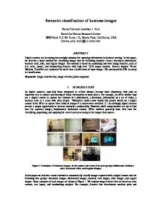
Forward, stepwise model selection resulted resulted in in model model fits fits for for Vanua Vanua Vatu Vatu with McFadden’s back reef, reef, fore fore reef, reef, and and land land models, models, respectively. respectively. R-squared values of 0.62, 0.72, and 0.57 for the back Detailed tables for Vanua Vatu showing likelihood ratio test results from the stepwise model selection Vatu process, and parameter estimates for the final back reef, for reef and terrestrial models, are provided in the supplementary materials that accompany this article. Figure 2a shows shows habitat habitatclass classassignments assignmentsmade madebybythe themodel model Vanua Vatu, comparison forfor Vanua Vatu, in in comparison to a map (Figure developed manually solely using contextual editing. Comparison of atomap (Figure 2b)2b) thatthat waswas developed manually solely using contextual editing. Comparison of the the test image objects set aside the training data, the with the model predictions forimage these test datadata image objects set aside from from the training data, with model predictions for these image objects, showed an overall accuracy of percent. 85 percent. error matricesand andaccuracy accuracy calculations objects, showed an overall accuracy of 85 TheThe error matrices (Tables 2 and 3) correlate to some of the areas where differences exist between algorithm and manual image object classifications classifications (Figure (Figure 2). 2). InInthe theback back reef zone Vanua Vatu, model tended reef zone of of Vanua Vatu, thethe model tended to to systematically over predict the placement of coral habitat where dense macroalgae stands systematically over predict the placement of coral habitat where dense macroalgae stands were located, and also confused back reef sediment, where rubble existed, and vice versa. On the fore reef, the model was essentially binomial as it was only trying to differentiate between coral and sediment. atat times difficult to to discern as Although spectrally and and texturally texturallyvery verydifferent, different,these thesetwo twoclasses classeswere were times difficult discern thethe fore-reef slopes to to depth because ofofthe as fore-reef slopes depth because thenear nearexponential exponentialattenuation attenuationofoflight lightby bywater. water. On land, the model was unable to differentiate man-made features, (defined as urban in Table 1), primarily confusing both of these classes with beach sand and unvegetated terrestrial areas. Therefore, in order to attain a meaningful accuracy, objects belonging to the urban class needed to be manually classified is worthy worthy of of note note that that urban urban landscapes landscapes are are notoriously difficult to identify via contextual editing. It is in visible-spectrum satellite imagery [85,86]. In addition, objects on land that were determined to be unvegetated terrestrial were often misclassified misclassified by by the the model model as as vegetated vegetated terrestrial. terrestrial.
15902 9
Remote Sens. 2015, 7, page–page 15894–15916
Figure 2. (a) Model predicted habitat classifications for objects in Vanua Vatu, Fiji. Note that areas Figure 2. (a) Model predicted habitat classifications for objects in Vanua Vatu, Fiji. Note that areas classified as deep ocean or reef crest were not predicted and were assigned during zone assignment as classified as deep ocean or reef crest were not predicted and were assigned during zone assignment described in Figure 1. In addition, note that object classifications assigned based on field observations as described in Figure 1. In addition, note that object classifications assigned based on field or classified because they were part of the training dataset are included in the figure. (b) Habitat observations or classified because they were part of the training dataset are included in the figure. classifications for Vanua Vatu, Fiji using a manual, contextual editing approach. The legend showing (b) Habitat classifications for Vanua Vatu, Fiji using a manual, contextual editing approach. which habitat type each color in the figure represents can be found in Table 1. The legend showing which habitat type each color in the figure represents can be found in Table 1.
Similar issues were identified in some of the other five sites that were mapped using discrete choice models. In Matuka (Figure 3), instance, the model systematically over predicted coral in Similar issues were identified in for some of the other five sites that were mapped using discrete areas where there were extensive seagrass meadows (seagrass producer error of 0.26 user error of 0.63) choice models. In Matuka (Figure 3), for instance, the model systematically over predicted coral in and missed coral in portions of the lagoon floor (lagoon coral producer error of 0.73 and user error areas where there were extensive seagrass meadows (seagrass producer error of 0.26 user error of of 0.71). previously discussed, model wasfloor not able to effectively identify fore flats 0.63) andAs missed coral in portions the of the lagoon (lagoon coral producer error ofreef 0.73sand and user (producer error of 0.06 and user error of 0.43), particularly when located close to the depth limit of the error of 0.71). As previously discussed, the model was not able to effectively identify fore reef sand sensor’s capability (about meters clear waters). However, in places forelimit reef flats (producer error of 0.0630and userin error oftropical 0.43), particularly when located closewhere to thethe depth was by a wider shelf and a gentle such as the east side of Tuvuca (Figure 4), of thecharacterized sensor’s capability (about 30 meters in cleargradient, tropical waters). However, in places where the fore the model more successfully identified the fore reef sand flats class (producer error of 0.71 and user reef was characterized by a wider shelf and a gentle gradient, such as the east side of Tuvuca error of 4), 0.80). urban features present on the peninsula of land theclass center of Figureerror 3, Matuka, (Figure the The model more successfully identified the fore reef sandinflats (producer of 0.71 were also not well defined by the model (producer error of 0.52 and user error of 0.68), though and user error of 0.80). The urban features present on the peninsula of land in the center of Figure in 3, this example, least the urban features accurately Most Matuka, were at also notsome wellof defined by the modelwere (producer erroridentified. of 0.52 and userdisconcertingly, error of 0.68), however, fact that the modelsome completely mangroves as terrestrial vegetation. though inwas thistheexample, at least of the misidentified urban features were accurately identified. Most
disconcertingly, however, was the fact that the model completely misidentified mangroves as terrestrial vegetation.
15903 10
Remote Sens. 2015, 7, 15894–15916
Table 2. Error matrix comparing model predicted habitats (rows) for test data image objects (one third of the training data set aside, and not used for model fitting) with the test data habitat assignments made using ground-truth data for Vanua Vatu. Values represent numbers of image objects. Habitat
Back Reef Coral
Rubble
Back Reef Sed.
Beach Sand
Back Reef Coral Rubble Back Reef Sediment Beach Sand Macroalgae Seagrass Fore Reef Sediment Fore Reef Coral Terrestrial Vegetation Unvegetated Terrestrial Urban Column Total
1006 99 31 0 1 4 0 0 0 0 0 1141
143 934 22 0 0 7 0 0 0 0 0 1106
23 27 113 0 0 2 0 0 0 0 0 165
0 0 0 196 0 0 0 0 1 27 0 224
Macro-Algae Sea-Grass 17 1 0 0 9 1 0 0 0 0 0 28
15904
11 5 0 0 3 69 0 0 0 0 0 88
Fore Reef Sed.
Fore Reef Coral
Terres. Veg.
Unveg. Terres.
Urban
Row Total
0 0 0 0 0 0 31 15 0 0 0 46
0 0 0 0 0 0 9 674 0 0 0 683
0 0 0 3 0 0 0 0 514 30 0 547
0 0 0 39 0 0 0 0 75 51 0 165
0 0 0 15 0 0 0 0 0 0 0 15
1200 1066 166 253 13 83 40 689 590 108 0 4208
Remote Sens. 2015, 7, page–page
Remote Sens. 2015, 7, 15894–15916 Table 3. User and producer accuracies calculated for Vanua Vatu from the error matrix in Table 2.
Habitat
Model Fit vs. Training Test Data
Table 3. User and producer accuracies calculated forUser Vanua Vatu fromProducer the error matrix in Table 2.
Back Reef Coral Habitat Rubble Back Reef Sediment Back Reef Coral Beach Sand Rubble Macroalgae Back Reef Sediment Beach Sand Seagrass Macroalgae Fore Reef Sediment Seagrass Reef Coral Fore ReefFore Sediment ForeTerrestrial Reef Coral Vegetation Terrestrial VegetationTerrestrial Unvegetated Unvegetated Terrestrial Urban Urban
0.84
0.88
0.68 0.77 0.69 0.83 0.78 0.98 0.87 0.47 0
0.68 0.88 0.88 0.84 0.32 0.68 0.88 0.78 0.32 0.67 0.78 0.99 0.67 0.94 0.99 0.94 0.31 00.31
Model Fit vs. Training Test Data 0.88 0.84 User Producer 0.84 0.88 0.68 0.77 0.69 0.83 0.78 0.98 0.87 0.47 0
0
Figure 3. (a) Model predicted habitat classifications for objects in a subsection of Matuka, Fiji. Note Figure 3. (a) Model predicted habitat classifications for objects in a subsection of Matuka, Fiji. Note that areas classified as deep ocean or reef crest were not predicted and were assigned during zone that areas classified as deep ocean or reef crest were not predicted and were assigned during zone assignment as described in Figure 1. In addition, note that object classifications assigned based on field assignment as described in Figure 1. In addition, note that object classifications assigned based on observations or classified because they were assigned as sample locations are included in the figure. field observations or classified because they were assigned as sample locations are included in the (b) Habitat classifications for a subsection of Matuka, Fiji determined using a manual, contextual figure. (b) Habitat classifications for a subsection of Matuka, Fiji determined using a manual, editing approach. The legend showing which habitat type each color in the figure represents can be contextual editing approach. The legend showing which habitat type each color in the figure found in Table 1. Note that for this location, the model overestimated the classification of lagoon represents can be found in Table 1. Note that for this location, the model overestimated the coral (red) and underestimated the classification of seagrass (light green). Similarly, the model had classification of lagoon coral (red) and underestimated the classification of seagrass (light green). difficulty classifying fore reef sediment (light yellow). Similarly, the model had difficulty classifying fore reef sediment (light yellow).
12 15905
Remote Sens. 2015, 7, 15894–15916 Remote Sens. 2015, 7, page–page
Figure 4. (a) (a) Model Model predicted predicted habitat habitat classifications for objects in Note that areas in Tuvuca, Tuvuca, Fiji. Fiji. Note classified as were assigned during zone assignment as as deep deep ocean oceanor orreef reefcrest crestwere werenot notpredicted predictedand and were assigned during zone assignment described in Figure 1. In addition, note thatnote object classifications assigned based on field observations as described in Figure 1. In addition, that object classifications assigned based on field or classified because they because were assigned as sample locations arelocations includedare in the figure.in(b) observations or classified they were assigned as sample included theHabitat figure. classifications for Tuvuca, Fiji determined using a manual, contextual editing approach. The legend (b) Habitat classifications for Tuvuca, Fiji determined using a manual, contextual editing approach. showing which habitat type each color in the figure can represents be found incan Table Note in that in this The legend showing which habitat type each colorrepresents in the figure be1.found Table 1. application model was able to model classifywas foreable reef to sediment yellow) better than locations. Note that inthe this application the classify(light fore reef sediment (lightother yellow) better
than other locations.
In Fulaga, Fiji (Figure 5), the model poorly identified the large swaths of macroalgae on the In floor Fulaga, Fiji (Figure 5), the of model identified the of large swaths of macroalgae on the the lagoon (producer’s accuracy 0.27 poorly and user’s accuracy 0.68). For this site, however, lagoon floor (producer’s accuracy of 0.27 and user’s accuracy of 0.68). For this site, however, the model did successfully distinguish coral in the lagoon, in particular small coral patches (i.e., so model“bommies”) did successfully distinguish coralofin0.75 theand lagoon, particular small Overall, coral patches (i.e.,the somodel called called (producer accuracy userin accuracy of 0.75). though, “bommies”) (producer of 0.75 and user accuracy of 0.75). Overall, though, the model was was particularly adept accuracy at delineating seagrass beds, and the coral to sediment and coral to rubble particularly adept at delineating seagrass beds, and the coral to sediment and coral to rubble interfaces, even in cases where patches of coral were very small. This is an important strength of interfaces, even cases where patches of coral were very small. This is an growth important strength[87], of the the model as it isininvariably very time consuming, because of their ornate structures to model as it is invariably very time consuming, because of their ornate growth structures [87], to manually delineate coral patches from sediment in the back reef and lagoon zones. manually delineate coral patches from sediment in the back reef and lagoon zones. Spatially, uncertainty in model predictions (Figure 6) was highest at habitat transition boundaries Spatially, in model (Figure 6) in was transitionareas boundaries (i.e., where oneuncertainty habitat graded into predictions another) and lowest thehighest middleatofhabitat homogeneous of the (i.e., where one habitat graded into another) and lowest in the middle of homogeneous areas of the consistent habitat. For the application of the model to Vanua Vatu, classifications that the model consistent habitat. For the application of the model to Vanua Vatu, classifications that the model did did not predict very well, such as areas in the imagery with man-made structures that should not predict very well, as such as areas in the where imagery with man-made structures that should have been have been classified urban, or areas macroalgae are located adjacent to coral, showed classified as urban, or areas where macroalgae are located adjacent to coral, showed higher higher uncertainty. uncertainty. Finally, using the semi-automated approach presented in this study decreased the amount of semi-automated approachhalf. presented in this studyof Vanua decreased time Finally, needed tousing create the habitat maps by approximately For example, the map Vatu,the an amount of time needed to create habitat maps by approximately half. For example, the map of area of 40 square kilometers, was produced in about three days using the semi-automated approach Vanua Vatu, an area of 40 kilometers, was produced about three contextual days usingediting. the semipresented, in comparison to square about six days if entirely produced in using manual automated approach presented, in comparison to about six days if entirely produced using manual contextual editing.
15906 13
Remote Sens. 2015, 7, page–page Remote Remote Sens. Sens. 2015, 2015, 7, 7, 15894–15916 page–page
Figure 5. (a) Model predicted habitat classifications for objects in Fulaga, Fiji. Note that areas classified Figure 5.(a)(a) Model predicted habitat classifications for objects in Fulaga, Fiji.thatNote that areas Figure Model predicted habitat classifications for objects in Fulaga, Fiji. Note areas classified as deep5.ocean or reef crest were not predicted and were assigned during zone assignment as described classified as deep ocean or reef crest were not predicted and were assigned during zone assignment as as ocean or addition, reef crest were and were assigned during zoneon assignment as described in deep Figure 1. In note not thatpredicted object classifications assigned based field observations or described in Figure 1. In addition, note that object classifications assigned based on field observations in Figure because 1. In addition, noteassigned that object classifications assigned based in onthe field observations or classified they were as sample locations are included figure. (b) Habitat or classified because they wereassigned assignedasassample samplelocations locationsare are included included in in the figure. figure. (b) Habitat classified because they were classifications for Fulaga, Fiji determined using a manual, contextual editingthe approach. (b) TheHabitat legend classifications for Fulaga, Fiji determined using a manual, contextual editing approach. The legend classifications Fulaga, Fijieach determined using a manual, contextual editinginapproach. Thethat legend showing whichfor habitat type color in the figure represents can be found Table 1. Note the showing which habitat type each color in the figure represents can be found in Table 1. Note that the showing which habitat type each color in the figure represents can be found in Table 1. Note that the model had difficulty classifying the macroalgae on the lagoon floor (purple), but was able to select model had difficulty classifying the macroalgae on the lagoon floor (purple), but was able to select out model had difficulty the macroalgae lagoon floor (purple), out a lot of small reef classifying structures inside the lagoonon (sothe called “bommies”) (red). but was able to select a lot of small reef structures inside the lagoon (so called “bommies”) (red). out a lot of small reef structures inside the lagoon (so called “bommies”) (red).
Figure Model classification classification uncertainty uncertainty for for Vanua Vanua Vatu, Figure 6. 6. Model Vatu, Fiji, Fiji, represented represented as as the the probability probability that that an an object classified incorrectly. Darker represent objects with classification uncertainty. Figure 6. Model classification uncertainty for Vanua Vatu, Fiji, represented as the probability that an object was was classified incorrectly. Darker colors colors represent objects with higher higher classification uncertainty. object was classified incorrectly. Darker colors represent objects with higher classification uncertainty.
14 15907 14
Remote Sens. 2015, 7, 15894–15916
4. Discussion Although segmentation models, such as those tendered by eCognition, are well-developed, attributing habitat classes to the image-objects that result from segmentation remains challenging to automate for coral reef environments, but is otherwise prohibitively time consuming if affected manually. In the face of the now commonly termed “coral reef crisis”, though, regional-scale high-resolution habitat maps have never been in greater demand, particularly since they form the basis for the process of marine spatial planning, a strategy which has found particular favor for coral conservation [88–93]. Against this backdrop, this study has shown that although some manual editing of key classes might still be desirable, application of a multinomial logistic model to assign the image-objects created by eCognition into habitats can rapidly yield accurate reef maps. Furthermore, unlike manual attribution of habitats, being computationally efficient, this automated strategy is limited neither by the spatial resolution of the pixels nor the extent of the imagery. These factors conspire to make the model accessible to appropriately trained reef managers, even those in developing regions and even those equipped with a moderate specification laptop computer. Although the technique did perform well overall, there were still issues with misclassifications. Most of these errors occurred at the interface between habitat types. This could, in part, have been caused by objects that were not cleanly segmented by eCognition and therefore consisted of mixed habitat types (the object version of a mixed pixel), or objects that actually contained mixed pixels, meaning pixels that themselves covered multiple habitat types. That is, the failure was due to the segmentation model as opposed to the attribution of the segments using the multinomial logistic model. In either case, object statistics (such as spectral, textural, size, and shape) for objects that contain mixed habitat types would have been skewed towards the class contributing to the majority share of the segment. This presented a challenge to the classification model as the model may have calculated reasonable probabilities for multiple different habitat types. In nature, habitats grade from one to another and therefore do not always adhere to the crisp boundaries maps used for marine spatial planning demand [94]. These gradations in the satellite imagery result from spatial and temporal heterogeneity in ecology that operate on scales finer than the pixel size of even the most capable satellite instruments (such as WV2). For simplicity, heterogeneity is typically characterized using a patch-mosaic model, where a landscape or seascape is a collection of discrete patches of habitat. In our example, the gradients between these boundaries were a main source of uncertainty in habitat classification; this was clearly captured in the uncertainty raster in the results. One of the gradients that the model found difficult to resolve was the transition from back reef coral to coral rubble. This is perhaps logical considering the fact that both classes consisted of coral detritus and although this was consolidated in the former and fragmented in the latter, the spectral response of the two habitats was inseparable in the comparatively broad spectral bands of the WV2, as compared, for instance, to a hyperspectral sensor [20,28,95–98]. A second gradient that the model found difficult to resolve in certain locations was the differentiation between macroalgae on sediment and coral framework. Again, such confusion is to be anticipated given the strong chlorophyll signature of both habitats in the visible wavelength [99,100]. In addition, if a reef had suffered significant coral mortality and had been overgrown by macroalgae, this structure may look similar to adjacent patches of macroalgae on sediment preventing the routine use of satellite imagery to detect coral bleaching [50,101–104]. Discerning these two habitat types using satellite remote sensing remain difficult, despite the fact that aerial photography and hyperspectral approaches have made advances in these areas [19,21,105,106]. Our own ground-truth data confirmed that separating algae on coral framework from framework that contained a high percentage of live coral cover was especially challenging. In this case, both structures shared the same reef-like geometry, precluding the use of characteristics such as habitat shape as a diagnostic feature.
15908
Remote Sens. 2015, 7, 15894–15916
The rapid attenuation of visible light with increasing water depth made it more difficult for the model to distinguish between habitats at deeper depths. This was particularly evident in the fore reef environment when trying to distinguish deep sand channels from deep reef habitat, and also on deep lagoon floors, when distinguishing between barren lagoon floor and coral habitat, or barren lagoon floor and macroalgae. In the fore reef environment, however, this did not always register by the model as increased uncertainty. This is likely because on the fore reef, the algorithm only had to distinguish between two different types of habitat, coral and sand, where most of the image objects on the fore reef were coral. Therefore, there was a good chance that the algorithm would “guess” the correct habitat type, especially at the outer edges of imagery detectability, where even sandy areas can appear dark like reef habitat. To this end, incorporating various combinations of band ratios was helpful for discerning habitat types in deeper waters, and these factors were typically determined to be statistically significant in the model. Band ratios provide an index of relative band intensity that enhances the spectral differences between the bands while reducing the effects of depth [107]. The five primary visible bands in the WorldView-2 satellite imagery offer a number of combinations of band ratios that can be used to help distinguish between habitat types [84]. Terrestrially, the model also had trouble distinguishing gradients. One area where this was a particular issue was between areas that our ground-truthing had determined to be vegetated versus unvegetated. This may have been because areas that contained exposed earth often had some low lying vegetative cover, such as low grasses, bushes, or other brush. Thus, such objects may actually have been mixed classes, consisting of some exposed soil, but not exclusively so, and therefore understandably difficult for the model to distinguish. As such, one change in the analysis that may have improved the classification could have been to split terrestrial vegetation into two classes, defining tree canopy and low grasslands or shrubs. Similarly, the model had a very difficult time distinguishing between terrestrial vegetation that contained tree canopy, and mangroves. Work has been done before successfully to distinguish mangroves from tree canopies of other species, and to discern different mangrove species from one another, however these efforts have largely utilized hyperspectral data which is more nimble at detecting subtle spectral differences or LiDAR which can key off of geometric differences in canopy structure [108–112]. These efforts have involved region-merging segmentation together with maximum likelihood, nearest-neighbor, and integrating pixel and object-based approaches, and receiver operating characteristic curve analysis [113,114]. Spectral analysis has been done to differentiate between several species [115,116]. Specifically, using WV2 satellite data, as used in this study, work has been done to characterize mangrove vegetation using semi-variograms combined with field data and visual image interpretation, looking at different object and pixel resolutions, and using support vector machines [117–119]. Due to the connectivity between mangrove habitat and the overall health of coral reefs and reef fish populations, future refinements of this model should try to incorporate elements from successful studies to improve the ability to distinguish mangrove canopy from that of other terrestrial tree species. Finally it is important to acknowledge that the need for an analyst to develop a training dataset to populate algorithms such as that presented in this paper, in the absence of an abundance of field data spanning the entire spatial domain, contains limitations. As discussed in the methodology, the purpose for developing and using a training dataset was to reduce the observation error associated with model fit and habitat prediction. Training datasets developed using expert judgement, however, even when grounded in some quantitative field data as in this study, are subject to both error and bias. Algorithm performance can naturally be improved if both the bias and error are reduced. Although models that fit the training data closely may have low bias, it does not necessarily mean that the estimated model parameters, which are then used to predict the classifications of all image objects, are error free. Furthermore, error from using a misspecified training dataset is passed on during model prediction, and this observation error is unable to be distinguished from model process error.
15909
Remote Sens. 2015, 7, 15894–15916
Therefore, training datasets must be developed with great care to ensure that observation error is as close to zero as possible. Along these same lines, the authors acknowledge that accuracy assessment typically compares results to field data, which are assumed to be 100% correct. However, due to the absence of an abundance of field data in this study, model results were compared to a test dataset defined as one third of the training dataset, which was set aside and not used to fit the models. In this case, the test dataset used for accuracy assessment was assumed to be 100% correct, which may not have been the case as per the discussion in the above paragraph. As such, the modelled results may have shared some biases with the training dataset, which are unable to be parsed out from the error matrices. 5. Conclusions Many coral reef cartographers face the challenge of having to map a large spatial area, using limited field samples, and the inability to automate the workflow. This leads to copious amounts of time spent manually producing maps or contextually editing products on which automated routines were not very successful. Despite the limitations described in this manuscript, using a multinomial logistic model to perform an initial automated pass at classifying coral reef habitat from satellite imagery was able to attain assignment accuracies exceeding 85 percent. This drastically reduced the time needed to produce the map, despite the need to still perform some contextual edits to correct some misclassifications. The probabilistic nature of the model provides for an estimation of uncertainty across space that can be provided to the end-user as a supplement to the habitat map. This is something that can only be provided using a statistically based approach and is not possible to provide when exclusively developing a map manually using contextual editing. Whether developing marine spatial planning scenarios or populating spatial models from reef habitat maps, an estimate of uncertainty across space is essential towards understanding the impact of proposed management efforts and ecological processes. In many cases, subtidal coral reef habitats of ecological and anthropogenic importance exist in remote locations that are financially and logistically difficult to access. Furthermore, most developing countries with coral reefs lack the resources necessary to conduct the extensive field campaigns that would make possible the collection of a comprehensively sampled ground-truth dataset. Yet, these places play central roles in protecting biodiversity and sustaining local economies by providing food, attracting tourism, and offering the coastline some shelter from storms, among other things. Due to the breadth of ecosystem services supplied by coral reefs, in addition to the anthropogenic stressors they face, the development of detailed maps is paramount to their effective management. As a result, if an informed analyst familiar with the reef system being mapped can make his or her best efforts to discern a training dataset and use this to produce a first version of a habitat map, this would at least provide a foundation with which the marine spatial planning process can begin. Further refinement of the map product can always be done by collecting additional field data and/or by obtaining additional input from individuals who live in communities adjacent to the reef system that is being studied. Acknowledgments: Financial support for this study and the accompanying fieldwork was provided by the National Coral Reef Institute (NCRI) and the Khaled bin Sultan Living Oceans Foundation (KSLOF). Invaluable logistical field support was provided by the crew of the M/Y Golden Shadow, through the generosity of HRH Prince Khaled bin Sultan. Thanks are extended to Brett Thomassie and DigitalGlobe Inc. for flexibility and unwavering assistance with acquiring Worldview-2 imagery. This is NCRI contribution 178. Author Contributions: Steven Saul conducted the analysis, and collected the field data. Both Steven Saul and Sam Purkis contributed to the writing of this manuscript. Sam Purkis provided valuable feedback on the early drafts of the manuscript. Conflicts of Interest: The authors declare no conflict of interest.
15910
Remote Sens. 2015, 7, 15894–15916
References 1.
2. 3.
4. 5. 6. 7. 8.
9.
10. 11. 12. 13. 14. 15. 16.
17. 18. 19.
20. 21.
Brander, L.M.; Eppink, F.V.; Schagner, P.; van Beukering, J.H.; Wagtendonk, A. GIS-based mapping of ecosystem services: The case of coral reefs. In Benefit Transfer of Environmental and Resource Values, The Economics of Non-Market Goods and Resources; Johnson, R.J., Rolfe, J., Rosenberger, R.S., Brouwer, R., Eds.; Springer: New York, NY, USA, 2015; Volume 14, pp. 465–485. Moberg, F.; Folke, C. Ecological goods and services of coral reef ecosystems. Ecol. Econ. 1999, 29, 215–233. [CrossRef] Done, T.J.; Ogden, J.C.; Wiebe, W.J.; Rosen, B.R. Biodiversity and ecosystem function of coral reefs. In Functional Roles of Biodiversity: A Global Perspective; Mooney, H.A., Cushman, J.H., Medina, E., Sala, O.E., Schulze, E., Eds.; Wiley: Chichester, UK, 1996; pp. 393–429. Shucksmith, R.; Lorraine, G.; Kelly, C.; Tweddle, J.R. Regional marine spatial planning—The data collection and mapping process. Mar. Policy 2014, 50, 1–9. [CrossRef] Shucksmith, R.; Kelly, C. Data collection and mapping—Principles, processes and application in marine spatial planning. Mar. Policy 2014, 50, 27–33. [CrossRef] Rowlands, G.; Purkis, S.J. Tight coupling between coral reef morphology and mapped resilience in the Red Sea. Mar. Pollut. Bull. 2016, 103, 1–23. Riegl, B.R.; Purkis, S.J. Coral population dynamics across consecutive mass mortality events. Glob. Chang. Biol. 2015, 21, 3995–4005. [CrossRef] [PubMed] Purkis, S.J.; Roelfsema, C. Remote sensing of submerged aquatic vegetation and coral reefs. In Wetlands Remote Sensing: Applications and Advances; Tiner, R., Lang, M., Klemas, V., Eds.; CRC Press—Taylor and Francis Group: Boca Raton, FL, USA, 2015; pp. 223–241. Rowlands, G.; Purkis, S.J.; Riegl, B.; Metsamaa, L.; Bruckner, A.; Renaud, P. Satellite imaging coral reef resilience at regional scale. A case-study from Saudi Arabia. Mar. Pollut. Bull. 2012, 64, 1222–1237. [CrossRef] [PubMed] Purkis, S.J.; Graham, N.A.J.; Riegl, B.M. Predictability of reef fish diversity and abundance using remote sensing data in Diego Garcia (Chagos Archipelago). Coral Reefs 2008, 27, 167–178. [CrossRef] Riegl, B.M.; Purkis, S.J.; Keck, J.; Rowlands, G.P. Monitored and modelled coral population dynamics and the refuge concept. Mar. Pollut. Bull. 2009, 58, 24–38. [CrossRef] [PubMed] Riegl, B.M.; Purkis, S.J. Model of coral population response to accelerated bleaching and mass mortality in a changing climate. Ecol. Model. 2009, 220, 192–208. [CrossRef] Purkis, S.J.; Riegl, B. Spatial and temporal dynamics of Arabian Gulf coral assemblages quantified from remote-sensing and in situ monitoring data. Mar. Ecol. Prog. Ser. 2005, 287, 99–113. [CrossRef] Mumby, P.J.; Gray, D.A.; Gibson, J.P.; Raines, P.S. Geographical information systems: A tool for integrated coastal zone management in Belize. Coast. Manag. 1995, 23, 111–121. [CrossRef] Rowlands, G.; Purkis, S.J.; Bruckner, A. Diversity in the geomorphology of shallow-water carbonate depositional systems in the Saudi Arabian Red Sea. Geomorphology 2014, 222, 3–13. [CrossRef] Purkis, S.J.; Kerr, J.; Dempsey, A.; Calhoun, A.; Metsamaa, L.; Riegl, B.; Kourafalou, V.; Bruckner, A.; Renaud, P. Large-scale carbonate platform development of Cay Sal Bank, Bahamas, and implications for associated reef geomorphology. Geomorphology 2014, 222, 25–38. [CrossRef] Schlager, W.; Purkis, S.J. Bucket structure in carbonate accumulations of the Maldive, Chagos and Laccadive archipelagos. Int. J. Earth Sci. 2013, 102, 2225–2238. [CrossRef] Glynn, P.W.; Riegl, B.R.; Purkis, S.J.; Kerr, J.M.; Smith, T. Coral reef recovery in the Galápagos Islands: The northern-most islands (Darwin and Wenman). Coral Reefs 2015, 34, 421–436. [CrossRef] Knudby, A.; Pittman, S.J.; Maina, J.; Rowlands, G. Remote sensing and modeling of coral reef resilience. In Remote Sensing and Modeling, Advances in Coastal and Marine Resources; Finkl, C.W., Makowski, C., Eds.; Springer: New York, NY, USA, 2014; pp. 103–134. Xu, J.; Zhao, D. Review of coral reef ecosystem remote sensing. Acta Ecol. Sin. 2014, 34, 19–25. [CrossRef] Mumby, P.J.; Skirving, W.; String, A.E.; Hardy, J.T.; LeDrew, E.F.; Hochberg, E.J.; Stumpf, R.P.; David, L.T. Remote sensing of coral reefs and their physical environment. Mar. Pollut. Bull. 2004, 48, 219–228. [CrossRef] [PubMed]
15911
Remote Sens. 2015, 7, 15894–15916
22.
23.
24. 25. 26. 27.
28. 29. 30. 31.
32. 33. 34. 35.
36. 37.
38.
39.
40.
41. 42. 43.
Bruckner, A.; Kerr, J.; Rowlands, G.; Dempsey, A.; Purkis, S.J.; Renaud, P. Khaled bin Sultan Living Oceans Foundation Atlas of Shallow Marine Habitats of Cay Sal Bank, Great Inagua, Little Inagua and Hogsty Reef, Bahamas; Panoramic Press: Phoenix, AZ, USA, 2015; pp. 1–304. Bruckner, A.; Rowlands, G.; Riegal, B.; Purkis, S.J.; Williams, A.; Renaud, P. Khaled bin Sultan Living Oceans Foundation Atlas of Saudi Arabian Red Sea Marine Habitats; Panoramic Press: Phoenix, AZ, USA, 2012; pp. 1–262. Mumby, P.J.; Clark, C.D.; Green, E.P.; Edwards, A.J. Benefits of water column correction and contextual editing for mapping coral reefs. Int. J. Remote Sens. 1998, 19, 203–210. [CrossRef] Andrefouet, S. Coral reef habitat mapping using remote sensing: A user vs. producer perspective, implications for research, management and capacity building. J. Spat. Sci. 2008, 53, 113–129. [CrossRef] Purkis, S.J.; Pasterkamp, R. Integrating in situ reef-top reflectance spectra with Landsat TM imagery to aid shallow-tropical benthic habitat mapping. Coral Reefs 2004, 23, 5–20. [CrossRef] Purkis, S.J.; Kenter, J.A.M.; Oikonomou, E.K.; Robinson, I.S. High-resolution ground verification, cluster analysis and optical model of reef substrate coverage on Landsat TM imagery (Red Sea, Egypt). Int. J. Remote Sens. 2002, 23, 1677–1698. [CrossRef] Karpouzli, E.; Malthus, T.J.; Place, C.J. Hyperspectral discrimination of coral reef benthic communities in the western Caribbean. Coral Reefs 2004, 23, 141–151. [CrossRef] Purkis, S.J. A “reef-up” approach to classifying coral habitats from IKONOS imagery. IEEE Trans. Geosci. Remote Sens. 2005, 43, 1375–1390. [CrossRef] Hochberg, E.J.; Atkinson, M.J.; Andréfouët, S. Spectral reflectance of coral reef bottom-types worldwide and implications for coral reef remote sensing. Remote Sens. Environ. 2003, 85, 159–173. [CrossRef] Andréfouët, S.; Kramer, P.; Torres-Pulliza, D.; Joyce, K.E.; Hochberg, E.J.; Garza-Pérez, R.; Mumby, P.J.; Riegl, B.; Yamano, H.; White, W.H.; et al. Multi-site evaluation of IKONOS data for classification of tropical coral reef environments. Remote Sens. Environ. 2003, 88, 128–143. [CrossRef] Goodman, J.; Ustin, S. Classification of benthic composition in a coral reef environment using spectral unmixing. J. Appl. Remote Sens. 2007, 1, 1–17. Purkis, S.J. Calibration of Satellite Images of Reef Environments. Ph.D. Thesis, Vrije Universiteit, Amsterdam, The Netherlands, June 2004. Hedley, J.D.; Mumby, P.J. A remote sensing method for resolving depth and subpixel composition of aquatic benthos. Limnol. Oceanogr. 2003, 48, 480–488. [CrossRef] Maeder, J.; Narumalani, S.; Rundquist, D.C.; Perk, R.L.; Schalles, J.; Hutchins, K.; Keck, J. Classifying and mapping general coral-reef structure using IKONOS data. Photogramm. Eng. Remote Sens. 2002, 68, 1297–1305. Hedley, J.; Harborne, A.; Mumby, P. Simple and robust removal of sun glint for mapping shallow-water benthos. Int. J. Remote Sens. 2005, 26, 2107–2112. [CrossRef] Hochberg, E.J.; Andréfouët, S.; Tyler, M.R. Sea surface correction of high spatial resolution Ikonos images to improve bottom mapping in near-shore environments. IEEE Trans. Geosci. Remote Sens. 2003, 41, 1724–1729. [CrossRef] Wedding, L.; Lepczyk, S.; Pittman, S.; Friedlander, A.; Jorgensen, S. Quantifying seascape structure: extending terrestrial spatial pattern metrics to the marine realm. Mar. Ecol. Prog. Ser. 2011, 427, 219–232. [CrossRef] Benfield, S.L.; Guzman, H.M.; Mair, J.M.; Young, J.A.T. Mapping the distribution of coral reefs and associated sublittoral habitats in Pacific Panama: A comparison of optical satellite sensors and classification methodologies. Int. J. Remote Sens. 2007, 28, 5047–5070. [CrossRef] Lunetta, R.S.; Congalton, R.G.; Fenstermaker, L.K.; Jensen, J.R.; McGwire, K.C.; Tinney, L.R. Remote sensing and geographic information systems data integration: Error sources and research ideas. Photogramm. Eng. Remote Sens. 1991, 53, 1259–1263. Shao, G.; Wu, J. On the accuracy of landscape pattern analysis using remote sensing data. Landsc. Ecol. 2008, 23, 505–511. [CrossRef] Foody, G.M. Harshness in image classification accuracy assessment. Int. J. Remote Sens. 2008, 29, 3137–3159. [CrossRef] Foody, G.M. Assessing the accuracy of land cover change with imperfect ground reference data. Remote Sens. Environ. 2010, 114, 2271–2285. [CrossRef]
15912
Remote Sens. 2015, 7, 15894–15916
44. 45. 46. 47.
48. 49. 50.
51.
52.
53. 54.
55. 56. 57. 58.
59. 60.
61. 62. 63. 64.
65.
Hochberg, E.J.; Atkinson, M.J. Spectral discrimination of coral reef benthic communities. Coral Reefs 2000, 19, 164–171. [CrossRef] Hogland, J.; Billor, N.; Anderson, N. Comparison of standard maximum likelihood classification and polytomous logistic regression used in remote sensing. Eur. J. Remote Sens. 2013, 46, 623–640. [CrossRef] Pal, M. Multinomial logistic regression-based feature selection for hyperspectral data. Int. J. Appl. Earth Obs. Geoinform. 2012, 14, 214–220. [CrossRef] Debella-Gilo, M.; Etzelmuller, B. Spatial prediction of soil classes using digital terrain analysis and multinomial logistic regression modeling integrated in GIS: examples from Vestfold County, Norway. Catena 2009, 77, 8–18. [CrossRef] Li, J.; Marpu, P.R.; Plaza, A.; Bioucas-Dias, J.M.; Benediktsson, J.A. Generalized composit kernel framework for hyperspectral image classification. IEEE Trans. Geosci. Remote Sens. 2013, 51, 4816–4829. [CrossRef] Pal, M.; Foody, G.M. Evaluation of SVM, RVM and SMLR for accurate image classification with limited ground data. IEEE J. Sel. Top. Appl. Earth Obs. Remote Sens. 2012, 5, 1344–1355. [CrossRef] Mishra, D.R.; Narumalani, S.; Rundquist, D.; Lawson, M.; Perk, R. Enhancing the detection and classification of coral reef and associated benthic habitats: a hyperspectral remote sensing approach. J. Geophys. Res. 2007, 112, 1–18. [CrossRef] Bernabé, S.; Marpu, P.R.; Plaza, A.; Mura, M.D.; Benediktsson, J.A. Spectral-spatial classification of multispectral images using kernal feature space representation. IEEE Geosci. Remote Sens. Lett. 2014, 11, 288–292. [CrossRef] Contreras-Silva, A.I.; López-Caloca, A.A.; Tapia-Silva, F.O.; Cerdeira-Estrada, S. Satellite remote sensing of coral reef habitat mapping in shallow waters at Banco Chinchorro Reefs, México: A classification approach. In Remote Sensing—Applications; Escalante, B., Ed.; InTech: Rijeka, Croatia, 2012; pp. 331–354. Purkis, S.J.; Myint, S.; Riegl, B. Enhanced detection of the coral Acropora cervicornis from satellite imagery using a textural operator. Remote Sens. Environ. 2006, 101, 82–94. [CrossRef] Holden, H.; Derksen, C.; LeDrew, E.; Wulder, M. An examination of spatial autocorrelation as a means of monitoring coral reef ecosystems. In Proceedings of the IEEE 2001 International Geoscience and Remote Sensing Symposium, Sydney, Australia, 9–13 July 2001; Volume 2, pp. 622–624. Keck, J.; Houston, R.S.; Purkis, S.J.; Riegl, B. Unexpectedly high cover of Acropora cervicornis on offshore reefs in Roatan (Honduras). Coral Reefs 2005, 24, 509. [CrossRef] LeDrew, E.F.; Holden, H.; Wulder, M.A.; Derksen, C.; Newman, C. A spatial operator applied to multidate satellite imagery for identification of coral reef stress. Remote Sens. Environ. 2004, 91, 271–279. [CrossRef] Roelfsema, C.; Phinn, S.; Jupiter, S.; Comley, J. Mapping coral reefs at reef to reef-system scales, 10s-1000s km2 , using object-based image analysis. Int. J. Remote Sens. 2013, 18, 6367–6388. [CrossRef] Roelfsema, C.; Phinn, S.; Jupiter, S.; Comley, J.; Beger, M.; Patterson, E. The application of object-based analysis of high spatial resolution imagery for mapping large coral reef systems in the West Pacific at geomorphic and benthic community scales. In Proceedings of the IEEE International Geoscience and Remote Sensing Symposium, Honolulu, HI, USA, 25–30 July 2010; Volume 11, pp. 4346–4349. Phinn, S.R.; Roelfsema, C.M.; Mumby, P.J. Multi-scale, object-based image analysis for mapping geomorphic and ecological zones on coral reefs. Int. J. Remote Sens. 2012, 33, 3768–3797. [CrossRef] Knudby, A.; Roelfsema, C.; Lyons, M.; Phinn, S.; Jupiter, S. Mapping fish community variables by integrating field and satellite data, object-based image analysis and modeling in a traditional Fijian fisheries management area. Remote Sens. 2011, 3, 460–483. [CrossRef] Harris, P.M.; Purkis, S.J.; Ellis, J. Analyzing spatial patterns in modern carbonate sand bodies from Great Bahama Bank. J. Sediment. Res. 2011, 81, 185–206. [CrossRef] Purkis, S.J.; Harris, P.M.; Ellis, J. Patterns of sedimentation in the contemporary Red Sea as an analog for ancient carbonates in rift settings. J. Sediment. Res. 2012, 82, 859–870. [CrossRef] Harris, P.M.; Purkis, S.J.; Ellis, J.; Swart, P.K.; Reijmer, J.J.G. Mapping water-depth and depositional facies on Great Bahama Bank. Sedimentology 2015, 62, 566–589. [CrossRef] Purkis, S.J.; Casini, G.; Hunt, D.; Colpaert, A. Morphometric patterns in Modern carbonate platforms can be applied to the ancient rock record: Similarities between Modern Alacranes Reef and Upper Palaeozoic platforms of the Barents Sea. Sediment. Geol. 2015, 321, 49–69. [CrossRef] Purkis, S.J.; Rowlands, G.P.; Riegl, B.M.; Renaud, P.G. The paradox of tropical karst morphology in the coral reefs of the arid Middle East. Geology 2010, 38, 227–230. [CrossRef]
15913
Remote Sens. 2015, 7, 15894–15916
66. 67.
68. 69.
70.
71. 72. 73.
74. 75. 76. 77. 78. 79. 80. 81. 82. 83. 84.
85. 86. 87. 88.
Peña, J.M.; Gutiérrez, P.A.; Hervás-Martínez, C.; Six, J.; Plant, R.E.; López-Granados, F. Object-based image classification of summer crops with machine learning methods. Remote Sens. 2014, 6, 5019–5041. [CrossRef] Vatsavai, R.R. High-resolution urban image classification using extended features. In Proceedings of the IEEE International Conferene on Data Mining Workshops, Vancouver, BC, USA, 11 December 2011; Volume 11, pp. 869–876. Zhang, C.; Xie, Z. Combining object-based texture measures with a neural network for vegetation mapping in the Everglades from hyperspectral imagery. Remote Sens. Environ. 2012, 124, 310–320. [CrossRef] Semi-automatic classification of tree species in different forest ecosystems by spectral and geometric variables derived from Airborne Digital Sensor (ADS40) and RC30 data. Remote Sens. Environ. 2011, 115, 76–85. Pant, P.; Heikkinen, V.; Korpela, I.; Hauta-Kasari, M.; Tokola, T. Logistic regression-based spectral band selection for tree species classification: Effects of spatial scale and balance in training samples. IEEE Geosci. Remote Sens. Lett. 2014, 11, 1604–1608. [CrossRef] Zhang, C.; Selch, D.; Xie, Z.; Roberts, C.; Cooper, H.; Chen, G. Object-based benthic habitat mapping in the Florida Keys from hyperspectral imagery. Estuar. Coastal Shelf Sci. 2013, 134, 88–97. [CrossRef] Zhang, C. Applying data fusion techniques for benthic habitat mapping and monitoring in a coral reef ecosystem. ISPRS J. Photogramm. Remote Sens. 2015, 104, 213–223. [CrossRef] Wahidin, N.; Siregar, V.P.; Nababan, B.; Jaya, I.; Wouthuyzen, S. Object-based image analysis for coral reef benthic hábitat mapping with several classification algorithms. Procedia Environ. Sci. 2015, 24, 222–227. [CrossRef] Jensen, J. Introductory Digital Image Processing: A Remote Sensing Perspective, 3rd ed.; Pearson Prentice Hall: Upper Saddle River, NJ, USA, 2005; pp. 1–526. Purkis, S.J.; Rowlands, G.; Kerr, J.M. Unravelling the influence of water depth and wave energy on the facies diversity of shelf carbonates. Sedimentology 2015, 62, 541–565. [CrossRef] MacFaden, D. Conditional logit analysis of qualitative choice behavior. In Frontiers in Econometrics; Zarembka, P., Ed.; Academic Press: New York, NY, USA, 1974; pp. 105–142. Train, K.E. Discrete Choice Methods with Simulation, 2nd ed.; Cambridge University Press: New Yok, NY, USA, 2009; pp. 1–75. Cawley, G.C.; Talbot, N.L.C. Gene selection in cancer classification using sparse logistic regression with Bayesian regularisation. Bioinformatics 2006, 22, 2348–2355. [CrossRef] [PubMed] Zhong, P.; Zhang, P.; Wang, R. Dynamic learning of SMLR for feature selection and classification of hyperspectral data. IEEE Geosci. Remote Sens. Lett. 2008, 5, 280–284. [CrossRef] Train, K.; Winston, C. Vehicle choice behavior and the declining market share of U.S. automakers. Int. Econom. Rev. 2007, 48, 1469–1496. [CrossRef] Train, K.; McFadden, D. The goods-leisure tradeoff and disaggregate work trip mode choice models. Transp. Res. 1978, 12, 349–353. [CrossRef] Smith, M.D. State dependence and heterogeneity in fishing location choice. J. Environ. Econom. Manag. 2005, 50, 319–340. [CrossRef] Burnham, K.P.; Anderson, D.R. Model Selection and Multinomial Inference: A Practical Information-Theoretic Approach, 2nd ed.; Springer: New York, NY, USA, 2002; pp. 41–96. Kerr, J.M. Worldview-2 Offers New Capabilities for the Monitoring of Threatened Coral Reefs. Available online: http://www.watercolumncorrection.com/documents/Kerr_2010_Bathymetry_from_WV2.pdf (accessed on 16 September 2015). Myint, S.W.; Wentz, L.; Purkis, S.J. Employing Spatial Metrics in Urban Land-use/Land-cover Mapping: Comparing the Getis and Geary Indices. Photogramm. Eng. Remote Sens. 2007, 73, 1403–1415. [CrossRef] Purkis, S.J.; Klemas, V. Remote Sensing and Global Environmental Change; Wiley-Blackwell: Oxford, UK, 2011; pp. 1–368. Schlager, W.; Purkis, S.J. Reticulate reef patterns´antecedent karst versus self-organization. Sedimentology 2015, 62, 501–515. [CrossRef] Roberts, C.M.; Andelman, S.; Branch, G.; Bustamante, R.H.; Castilla, J.C.; Dugan, J.; Halpern, B.S.; Lafferty, K.D.; Leslie, H.; Lubchenco, J.; et al. Ecological criteria for evaluating candidate sites for marine reserves. Ecol. Appl. 2003, 13, 199–214. [CrossRef]
15914
Remote Sens. 2015, 7, 15894–15916
89. 90. 91. 92.
93. 94.
95. 96. 97. 98. 99. 100.
101. 102. 103. 104. 105.
106. 107. 108. 109. 110.
111.
Ward, T.J.; Vanderklift, M.A.; Nicholls, A.O.; Kechington, R.A. Selecting marine reserves using habitats and species assemblages as surrogates for biological diversity. Ecol. Appl. 1999, 9, 691–698. [CrossRef] Stevens, T.; Connolly, R.M. Local-scale mapping of benthic habitats to assess representation in a marine protected area. Mar. Freshw. Res. 2004, 56, 111–123. [CrossRef] Pittman, S.J.; Kneib, R.T.; Simenstad, C.A. Practicing coastal seascape ecology. Mar. Ecol. Prog. Ser. 2011, 427, 187–190. [CrossRef] Mumby, P.J.; Broad, K.; Brumbaugh, D.R.; Dahlgren, C.P.; Harborne, A.R.; Hastings, A.; Holmes, K.E.; Kappel, C.V.; Micheli, F.; Sanchirico, J.N. Coral reef habitats as surrogates of species, ecological functions, and ecosystem services. Conserv. Biol. 2008, 22, 941–951. [CrossRef] [PubMed] Murphy, H.M.; Jenkinsm, G.P. Observational methods used in marine spatial monitoring of fishes and associated habitats: a review. Mar. Freshw. Res. 2009, 61, 236–252. [CrossRef] Cushman, S.A.; Gutzweiler, K.; Evans, J.S.; McGarigal, K. The gradient paradigm: a conceptual and analytical framework for landscape ecology. In Spatial Complexity, Informatics, and Wildlife Conservation; Huettmann, F., Cushman, S.A., Eds.; Springer: New York, NY, USA, 2009; pp. 83–107. Mumby, P.J.; Hedley, J.D.; Chisholm, J.R.M.; Clark, C.D.; Ripley, H.; Jaubert, J. The cover of living and dead corals from airborne remote sensing. Coral Reefs 2004, 23, 171–183. [CrossRef] Kutser, T.; Miller, I.; Jupp, D.L.B. Mapping coral reef benthic substrates using hyperspectral space-borne images and spectral libraries. Estuarine Coast. Shelf Sci. 2006, 70, 449–460. [CrossRef] Goodman, J.; Ustin, S.L. Classification of benthic composition in a coral reef environment using spectral unmixing. J. Appl. Remote Sens. 2007, 1, 1–17. Torres-Madronero, M.C.; Velez-Reyes, M.; Goodman, J.A. Subsurface unmixing for benthic habitat mapping using hyperspecgtral imagery and lidar-derived bathymetry. Proc. SPIE 2014, 9088, 90880M:1–90880M:15. Blaschke, T. Object based image analysis for remote sensing. ISPRS J. Photogramm. Remote Sens. 2010, 65, 2–16. [CrossRef] Benz, U.C.; Hofmann, P.; Willhauck, G.; Lingenfelder, I.; Heynen, M. Multi-resolution, object-oriented fuzzy analysis of remote sensing data for GIS-ready information. ISPRS J. Photogramm. Remote Sens. 2004, 58, 239–258. [CrossRef] Kutser, T.; Skirving, W.; Parslow, J.; Clementson, L.; Done, T.; Wakeford, M.; Miller, I. Spectral discrimination of coral reef bottom types. Geosci. Remote Sens. Symp. 2001, 6, 2872–2874. Barott, K.; Smith, J.; Dinsdale, E.; Hatay, M.; Sandin, S.; Rohwer, F. Hyperspectral and Physiological Analyses of Coral-Algal Interactions. PLoS ONE 2009, 4, e8043. [CrossRef] [PubMed] Myers, M.R.; Hardy, J.T.; Mazel, C.H.; Dustan, P. Optical spectra and pigmentation of Caribbean reef corals and macroalgae. Coral Reefs 1999, 18, 179–186. [CrossRef] Rowlands, G.P.; Purkis, S.J.; Riegl, B.M. The 2005 coral-bleaching event Roatan (Honduras): Use of pseudo-invariant features (PIFs) in satellite assessments. J. Spat. Sci. 2008, 53, 99–112. [CrossRef] Mumby, P.J.; Harborne, A.R. Development of a systematic classification scheme of marine habitats to facilitate regional management and mapping of Caribbean coral reefs. Biol. Conserv. 1999, 88, 155–163. [CrossRef] Joyce, K.E. A Method for Mapping Live Coral Cover Using Remote Sensing. Ph.D Thesis, The University of Queensland, Queensland, Australia, 2005. Stumpf, R.; Holderied, K.; Sinclair, M. Determination of water depth with high-resolution satellite imagery over variable bottom types. Limnol. Oceanogr. 2003, 48, 547–556. [CrossRef] Heumann, B.W. Satellite remote sensing of mangrove forests: Recent advances and future opportunities. Prog. Phys. Geogr. 2011, 35, 87–108. [CrossRef] Kuenzer, C.; Buemel, A.; Gebhardt, S.; Zuoc, T.V.; Dech, S. Remote sensing of mangrove ecosystems: A review. Remote Sens. 2011, 3, 878–928. [CrossRef] Simard, M.; Zhang, K.; Rivera-Monroy, V.H.; Ross, M.S.; Ruiz, P.L.; Castañeda-Moya, E.; Twilley, R.; Rodriguez, E. Mapping height and biomass of mangrove forests in Everglades National Park with SRTM elevation data. Photogramm. Eng. Remote Sens. 2006, 3, 299–311. [CrossRef] Zhang, K. Identification of gaps in mangrove forests with airborne LIDAR. Remote Sens. Environ. 2008, 112, 2309–2325. [CrossRef]
15915
Remote Sens. 2015, 7, 15894–15916
112. Knight, J.M.; Dale, P.E.R.; Spencer, J.; Griffin, L. Exploring LiDAR data for mapping the micro-topography and tidal hydro-dynamics of mangrove systems: an example from southeast Queensland, Australia. Estuar. Coast. Shelf Sci. 2009, 85, 593–600. [CrossRef] 113. Wang, L.; Sousa, W.P.; Gong, P. Integration of object-based and pixel-based classification for mapping mangroves with IKONOS imagery. Int. J. Remote Sens. 2004, 25, 5655–5668. [CrossRef] 114. Alatorre, L.C.; Sánchez-Andrés, R.; Cirujano, S.; Beguería, S.; Sánchez-Carrillo, S. Identification of mangrove areas by remote sensing: The ROC curve technique applied to the northwestern Mexico Coastal Zone using Landsat imagery. Remote Sens. 2011, 3, 1568–1583. [CrossRef] 115. Rebelo-Mochel, F.; Ponzoni, F.J. Spectral characterization of mangrove leaves in the Brazilian Amazonian Coast: Turiacu Bay, Maranhao State. Ann. Braz. Acad. Sci. 2007, 79, 683–692. [CrossRef] 116. Kamaruzaman, J.; Kasawani, I. Imaging spectrometry on mangrove species identification and mapping in Malaysia. WSEAS Trans. Biol. Biomed. 2007, 8, 118–126. 117. Kamal, M.; Phinn, S.; Johansen, K. Characterizing the spatial structure of mangrove features for optimizing image-based mangrove mapping. Remote Sens. 2014, 6, 984–1006. [CrossRef] 118. Kamal, M.; Phinn, S.; Johansen, K. Extraction of multi-scale mangrove features from WorldView-2 image data: an object-based image analysis approach. In Proceedings of the 34th Asian Conference on Remote Sensing, Bali, Indonesia, 20–24 October 2013; Volume 34, pp. 653–659. 119. Heenkenda, M.K.; Joyce, K.E.; Maier, S.W.; Bartolo, R. Mangrove species identification: Comparing WorldView-2 with aerial photographs. Remote Sens. 2014, 6, 6064–6088. [CrossRef] © 2015 by the authors; licensee MDPI, Basel, Switzerland. This article is an open access article distributed under the terms and conditions of the Creative Commons by Attribution (CC-BY) license (http://creativecommons.org/licenses/by/4.0/).
15916