remote sensing Article
Semi-Automatic Mapping of Tidal Cracks in the Fast Ice Region near Zhongshan Station in East Antarctica Using Landsat-8 OLI Imagery Fengming Hui 1 , Xinqing Li 1 , Tiancheng Zhao 1 , Mohammed Shokr 2 , Petra Heil 3 , Jiechen Zhao 4 , Yan Liu 1 , Shunlin Liang 5 and Xiao Cheng 1, * 1
2 3 4 5
*
State Key Laboratory of Remote Sensing Science, and College of Global Change and Earth System Science, and Joint Center for Global Change Studies, Beijing Normal University, Beijing 100875, China;
[email protected] (F.H.);
[email protected] (X.L.);
[email protected] (T.Z.);
[email protected] (Y.L.) Science and Technology Branch, Environment Canada, Toronto, ON M3H5T4, Canada;
[email protected] Australian Antarctic Division and Antarctic Climate and Ecosystems Cooperative Research Centre, University of Tasmania, Hobart, Tasmania 7001, Australia;
[email protected] Key Laboratory of Research on Marine Hazards Forecasting (SOA), National Marine Environmental Forecasting Center, Beijing 100081, China;
[email protected] Department of Geographical Sciences, University of Maryland, College Park, MD 20742, USA;
[email protected] Correspondence:
[email protected]; Tel.: +86-10-5880-2116
Academic Editors: Walt Meier and Prasad S. Thenkabail Received: 16 July 2015; Accepted: 7 March 2016; Published: 12 March 2016
Abstract: Tidal cracks are linear features that appear parallel to coastlines in fast ice regions due to the actions of periodic and non-periodic sea level oscillations. They can influence energy and heat exchange between the ocean, ice, and atmosphere, as well as human activities. In this paper, the LINE module of Geomatics 2015 software was used to automatically extract tidal cracks in fast ice regions near the Chinese Zhongshan Station in East Antarctica from Landsat-8 Operational Land Imager (OLI) data with resolutions of 15 m (panchromatic band 8) and 30 m (multispectral bands 1–7). The detected tidal cracks were determined based on matching between the output from the LINE module and manually-interpreted tidal cracks in OLI images. The ratio of the length of detected tidal cracks to the total length of interpreted cracks was used to evaluate the automated detection method. Results show that the vertical direction gradient is a better input to the LINE module than the top-of-atmosphere (TOA) reflectance input for estimating the presence of cracks, regardless of the examined resolution. Data with a resolution of 15 m also gives better results in crack detection than data with a resolution of 30 m. The statistics also show that, in the results from the 15-m-resolution data, the ratios in Band 8 performed best with values of the above-mentioned ratio of 50.92 and 31.38 percent using the vertical gradient and the TOA reflectance methods, respectively. On the other hand, in the results from the 30-m-resolution data, the ratios in Band 5 performed best with ratios of 47.43 and 17.8 percent using the same methods, respectively. This implies that Band 8 was better for tidal crack detection than the multispectral fusion data (Bands 1–7), and Band 5 with a resolution of 30 m was best among the multispectral data. The semi-automatic mapping of tidal cracks will improve the safety of vehicles travel in fast ice regimes. Keywords: tidal cracks; remote sensing; fast ice; Landsat-8 OLI
Remote Sens. 2016, 8, 242; doi:10.3390/rs8030242
www.mdpi.com/journal/remotesensing
Remote Sens. 2016, 8, 242
2 of 16
1. Introduction A crack is a form of fracture in the sea ice cover, manifested as an opening that exposes the underlying ocean to the atmosphere. The ocean water may freeze instantly if the temperature is cold enough. This discontinuity feature occurs during the breaking, rupturing, or thermal expansion (compression) of the ice cover [1]. Cracks can not only influence the growth and decay of sea ice, thus affecting the exchange of gas, energy, and heat at the ocean-ice-atmosphere interface [1–3], but can also provide important habitats for marine mammals, such as Weddell seals [4,5] and access to hunting grounds for penguins [6,7]. Crack classifications have been summarized according to different characteristics, such as morphological indications, load applications affecting the ice cover, and genetic indications [1]. Tidal cracks are a type of crack, regardless of classification, and form in fast ice due to the actions of periodic and non-periodic sea level oscillations, which causes the ice surface to rise and fall and thus move apart and close, as ice is not known for its elastic properties. The cracks usually reoccur at the same location every year and are influenced by the bathymetry and tidal zone dynamics. They often appear parallel to the coastline as linear features [1,8]. The width of a tidal crack can range from a few centimeters to 1 m, while the length can reach a few kilometers [8]. Tidal cracks are considered hazardous conditions for human activities when crossing them because of their unstable ice thickness on both sides [1,9,10]. Tidal crack detection in fast ice has been studied in field surveys and remote sensing studies [9,11]. During field surveys, a tidal crack’s location, shape, length, and width, as well as the sea ice thickness, are often measured. The Chinese National Antarctic Research Expedition (CHINARE) has been conducting field surveys of tidal cracks in the fast ice near Zhongshan Station in East Antarctica every November since 1989, mainly to protect people/over ice vehicles from the danger posed by tidal cracks along transportation and resupply routes. In remote sensing data, tidal cracks could be identified using: (1) aerial photography [1]; (2) one-day interferograms generated from the ERS satellites tandem mission data [12]; and (3) visual analysis of image radar data (SAR data) [10]. Remote sensing images could use either one or both of the following criteria to identify the cracks: (1) their radiometric contrast against the surrounding ice; and (2) their distinct linear features. Linear feature extraction for roads, rivers, bridges, ridges, geological faults, and fractures in mountain crests using remotely sensed images has been conducted in numerous studies [13]. They employ one of three approaches: manual image interpretation, semi-automatic (computer-assisted) extraction, and automatic extraction, each of which has its own advantages [13–15]. One of the commonly used earth observation satellites in a wide range of applications is Landsat-8, which was successfully launched in February 2013 with its Operational Land Imager (OLI) and Thermal Infrared Sensor (TIRS). Up to this study the capability of OLI data for detection of tidal crack mapping has not yet been investigated. The OLI sensor has spatial and spectral characteristics well suited for characterizing snow/ice and water, and it provides a good areal coverage (a swath width of 185 km and revisit period of 16 days) for sea ice monitoring. Here, we employed the automatic lineament extraction algorithm in Geomatica 2015 software (PCI Geomatics Inc., Markham, ON, Canada) to map tidal cracks in the fast ice near Zhongshan Station in East Antarctica in the early austral summer of 2013–2014. The purpose of the study was to investigate the capability of each band of OLI image to detect tidal cracks and length. The width of tidal cracks was not considered in this study since estimating this requires spatial resolution of remotely sensed data finer than the crack width (generally at least 0.2 m). It is anticipated that our findings will help research expeditions such as CHINARE to avoid risks while traveling on fast ice during the annual resupply of Antarctica stations, or during field activities to study the habitats of seals and penguins. 2. CHINARE and Study Area CHINARE began in 1984 and has been carried out successfully for 31 years. Currently, there are four Chinese Research Stations in Antarctica: Great Wall Station (62˝ 121 592 S, 58˝ 571 522 W, built in February 1985), Zhongshan Station (69˝ 221 242 S, 76˝ 221 402 E, built in February 1989), Kunlun Station
Remote Sens. 2016, 8, 242
3 of 16
1 012 S, 77˝ 061 582 (80˝ 25 Remote Sens. 2016, 8, 242
E, built in January 2009), and Taishan Station (73˝ 511 502 S, 76˝ 581 292 E, built 3 of 16 in February 2013) (Figure 1). The first two stations operate all year, and the latter two stations only operate during the austral summer because of severe weather conditions. RV Xuelong, currently only operate during the austral summer because of severe weather conditions. RV Xuelong, an icebreaker ice-strengthened to Class B1, is the only Chinese polar scientific research vessel. It was an icebreaker ice-strengthened to Class B1, is the only Chinese polar scientific research vessel. It was designed to break ice as thick as 1.1 m (including 0.2-m-thick snow) at 1.5 knots. Every year, RV designed to break ice as thick as 1.1 m (including 0.2-m-thick snow) at 1.5 knots. Every year, RV Xuelong Xuelong must traverse the pack ice in Prydz Bay (mostly fast ice) in East Antarctica and break through must traverse the pack ice in Prydz Bay (mostly fast ice) in East Antarctica and break through it to reach it to reach Zhongshan Station for resupply and staff transfer in late November or early December. Zhongshan Station for resupply and staff transfer in late November or early December. In general, In general, the shortest route through fast ice that RV Xuelong must cross to reach Zhongshan Station the shortest route through fast ice that RV Xuelong must cross to reach Zhongshan Station in early in early summer is approximately 10 km. Tidal cracks often appear in fast ice, posing dangers to snow summer is approximately 10 km. Tidal cracks often appear in fast ice, posing dangers to snow vehicles/snowmobiles along the travel route for resupply from RV Xuelong to Zhongshan Station. vehicles/snowmobiles along the travel route for resupply from RV Xuelong to Zhongshan Station.
Figure1.1. Map Map of of the the Antarctica Antarctica showing showing the four Chinese Figure Chinese stations. stations. The black black box box over over Zhongshan Zhongshan Stationshow showPrydz PrydzBay Baywhere wherethe thestudy studywas wasconducted. conducted. Station
The near Zhongshan Zhongshan Station Station in in Antarctica Antarctica (Figure (Figure 1). 1). Fast Fast ice ice isis Thestudy studyarea areaisis the the fast fast ice ice region region near adjacent for example, example, adjacentto tocoasts, coasts,islands, islands,or orgrounded grounded icebergs icebergs and and characterized characterized as as motionless motionless unless, unless, for ititbreaks by strong winds [16]. Its spatiotemporal patterns differ significantly and can extend from aa breaks by strong winds [16]. Its spatiotemporal patterns differ significantly and can extend from few meters to toaafew fewtens tens kilometers (although it reach can reach 200[17,18]. km) [17,18]. The few hundred hundred meters of of kilometers (although it can up toup 200to km) The extent extent theice fast ice Zhongshan near Zhongshan Station can be more 20in km in November, the maximum of the of fast near Station can be more than than 20 km November, and and the maximum ice ice thickness can reach 1.74 m [19]. The bathymetry near Zhongshan Station is highly undulated, thickness can reach 1.74 m [19]. The bathymetry near Zhongshan Station is highly undulated, which which can result in icebergs grounding offshore from Zhongshan Station. Both icebergs with different can result in icebergs grounding offshore from Zhongshan Station. Both icebergs with different sizes sizes and shapes and the nearby islands off Zhongshan Station allow fast ice to easily form, and tidal and shapes and the nearby islands off Zhongshan Station allow fast ice to easily form, and tidal cracks cracks are often observed. are often observed. 3.3.Data DataSet Setand andPre-Processing Pre-Processing OLI region off off Zhongshan Zhongshan Station Station was was OLIdata dataacquired acquired on on 30 30 November November 2014 2014 covering covering a fast ice region utilized 2).2). The data were freely downloaded in GeoTIFF format from the utilizedtotodetect detecttidal tidalcracks cracks(Figure (Figure The data were freely downloaded in GeoTIFF format from U.S. Geological Survey (USGS) website. Images werewere geometrically and and radiometrically corrected and the U.S. Geological Survey (USGS) website. Images geometrically radiometrically corrected projected in theinWGS1984/Antarctic PolarPolar Stereographic Projection. The spectral bands of the and projected the WGS1984/Antarctic Stereographic Projection. The spectral bands of OLI the sensor are given in Table 1. In 1. this multi-spectral bands in the (VNIR) and OLI sensor are given in Table Instudy, this study, multi-spectral bands in visible/near-infrared the visible/near-infrared (VNIR) shortwave infrared (SWIR)(SWIR) spectralspectral bands (Bands 1–7) with a spatial of 30 m, asofwell as the and shortwave infrared bands (Bands 1–7) with aresolution spatial resolution 30 m, as panchromatic band (Band band 8) with a spatial resolution 15 m, were for tidal detection. well as the panchromatic (Band 8) with a spatial of resolution of 15used m, were usedcrack for tidal crack The geographic accuracy for OLI data is about 12 m (according to Landsat-8 data products descriptions), which is less than one pixel. The OLI data was processed into top-of-atmosphere (TOA) reflectance according to the Landsat 8 Product specification. To obtain multispectral bands with a resolution of 15 m, the Gram–Schmidt spectral sharpening (GS) method [20] was employed for data
Remote Sens. 2016, 8, 242
4 of 16
detection. The geographic accuracy for OLI data is about 12 m (according to Landsat-8 data products descriptions), which is less than one pixel. The OLI data was processed into top-of-atmosphere (TOA) reflectance according to the Landsat 8 Product specification. To obtain multispectral bands with a Remote Sens. 2016, 8, 242 4 of 16 resolution of 15 m, the Gram–Schmidt spectral sharpening (GS) method [20] was employed for data fusion processing. Both panchromatic sharpening results Band 1–7 and Band 8 with a resolution fusion processing. Both thethe panchromatic sharpening results of of Band 1–7 and Band 8 with a resolution of m 15and m and multispectral Band with a resolution of 30 m are utilized tidal crack detections. of 15 thethe multispectral Band 1–71–7 with a resolution of 30 m are utilized forfor tidal crack detections.
Figure A false color image of combining Bands 3 and 2 (RGB) of the OLI data at 15-m resolution, Figure 2. A2.false color image of combining Bands 4, 34,and 2 (RGB) of the OLI data at 15-m resolution, acquired on 30 November 2014. The blue lines are overlaid tidal cracks identified visually in acquired on 30 November 2014. The blue lines are overlaid tidal cracks identified visuallythe inimage, the the lines with number labels (6 lines) are cracks confirmed based on field observations conducted image, the lines with number labels (6 lines) are cracks confirmed based on field observationson 30 and 31 2014. conducted onOctober 30 and 31 October 2014. Table 1. OLI and TIRS Bands of Landsat Table 1. OLI and TIRS Bands of Landsat 8. 8.
Band IDID Spectral Name Wavelength (m) Band Spectral Name Wavelength(µm) (µm) Resolution Resolution (m) Band 1 Coastal/aerosol 0.43–0.45 30 Band 1 Coastal/aerosol 0.43–0.45 30 Band 2 2 Blue 0.45–0.51 30 30 Band Blue 0.45–0.51 Band Green 0.53–0.59 Band 3 3 Green 0.53–0.59 30 30 Band 4 Red 0.64–0.67 Band 4 Red 0.64–0.67 30 30 Band 5 Near Infrared (NIR) 0.85–0.88 30 Band 5 Near Infrared (NIR) 0.85–0.88 30 30 Band 6 SWIR 1 1.57–1.65 Band 6 7 SWIR 12 1.57–1.65 30 30 Band SWIR 2.11–2.29 Band Panchromatic 0.50–0.68 Band 7 8 SWIR 2 2.11–2.29 30 15 Band Cirrus 1.36–1.38 Band 8 9 Panchromatic 0.50–0.68 15 30 Band 10 Thermal Infrared (TIRS) 1 10.60–11.19 Band 9 Cirrus 1.36–1.38 30 (30 *) 100 Band 11 Thermal Infrared (TIRS) 2 11.50–12.51 Band 10 Thermal Infrared (TIRS) 1 10.60–11.19 100 (30data *) product. * TIRS bands are acquired at a resolution of 100 m but are resampled to 30 m in the delivered Band 11 Thermal Infrared (TIRS) 2 11.50–12.51 * TIRS bands are acquired at a resolution of 100 m but are resampled to 30 m in the delivered data product.
vertical direction gradient data were obtained from filtered results OLI data Sobel TheThe vertical direction gradient data were obtained from thethe filtered results of of OLI data byby Sobel vertical direction operator with 3 windows [21]. A gradient image represents change the vertical direction operator with 3 ×33ˆwindows [21]. A gradient image represents thethe change inin the pixel values a given direction. most common is in edge detection. a gradient image, pixels pixel values in aingiven direction. Its Its most common useuse is in edge detection. In In a gradient image, pixels with largest gradient values identify edge pixels where edge can traced thedirection direction with thethe largest gradient values identify edge pixels where thethe edge can bebe traced inin the perpendicular to the gradient direction. In the current study, found that most tidal cracksare are perpendicular to the gradient direction. In the current study, wewe found that most tidal cracks parallel to the coastline in an east-west direction. This is almost parallel to the orientation of the image swath, so the vertical direction gradient data were used as the input image to detect tidal cracks. Visual extraction of tidal cracks was also implemented using available TOA reflectance and its gradient in the imagery data. Analysis was performed by sea ice experts at Beijing Normal University. In situ measurements were also conducted by wintering personnel of the 30th CHINARE on 30 and 31 October 2014 to identify and validate cracks. The measurements included snow depth, sea ice
Remote Sens. 2016, 8, 242
5 of 16
parallel to the coastline in an east-west direction. This is almost parallel to the orientation of the image swath, so the vertical direction gradient data were used as the input image to detect tidal cracks. Visual extraction of tidal cracks was also implemented using available TOA reflectance and its gradient in the imagery data. Analysis was performed by sea ice experts at Beijing Normal University. In situ measurements were also conducted by wintering personnel of the 30th CHINARE on 30 and 31 October 2014 to identify and validate cracks. The measurements included snow depth, sea ice thickness, crack points location (longitude and latitude), and the approximate length of each crack. Snow depth was measured by a stainless ruler with an accuracy of 0.1 cm, and sea ice thickness was measured by a special gage with an accuracy of 0.1 cm in holes drilled by a Kovacs ice auger (5 cm in diameter). Six tidal cracks with a width of 0.3–1.45 m were obtained from field observations, and 39 tidal cracks were identified from OLI data. The GPS measurements of the six tidal cracks could well coincide with those in the OLI image. Both sets (visually-interpreted cracks from the images and field-observed cracks) were used to evaluate the results from the semi-automatic mapping technique. Tidal prediction data for Zhongshan Station were obtained from the Australian Bureau of Meteorology for the analysis of the influence on the widths of tidal cracks. 4. Method 4.1. Manual Detection of Tidal Cracks in the Images Tidal cracks were detected manually in each one of the two OLI imagery data sets—the 15- and 30-m-resolution sets. The process involved manual interpretation of the images yet supported by field observations. It should be noted that narrow cracks may not be readily visible in the images since the resolution of the imagery data is coarser than the crack width. For this reason, field observations are used to confirm identification of those cracks which can hardly be seen in the image. Eventually, all cracks were identified manually in the images. Figure 2 is a false color OLI image (RGB assigned to bands 4, 3 and 2) at 30-m resolution, representing fast ice in the Prydz Bay. Manually detected tidal cracks are overlaid (blue lines). Two buffers were established using ArcGIS 10.0 software (ESRI In, Redlands, CA, USA); one included the detected crack pixels in the 15-m-resolution images and the other included the pixels in the 30-m-resolution images. In order to tolerate errors in the geo-location of the pixels, each buffer was enlarged to accommodate 3 pixels surrounding each detected pixel. Hence, the first and the second buffers tolerated errors within a width of 45 and 90 m, respectively. 4.2. The Automatic Lineament Extraction Algorithm An edge in an image represents a sharp local change in the image intensity, usually associated with a discontinuity (or equivalently high first derivative of the image intensity). Its shape usually depends on the geometrical and optical properties of the object, the illumination conditions, and the noise level in the images [22]. Tidal cracks can be considered edges because the seawater or the refrozen (new) ice within the crack can induce a difference in the spectral reflectance or backscatter density compared to the surrounding fast ice. This is how a tidal crack can be visually or automatically identified in remote sensing images even as at a subpixel level, albeit with inherent uncertainties. Previous studies have demonstrated good results in mapping linear discontinuities from satellite images [23–26]. The automatic lineament extraction algorithm in Geomatica 2015 software, integrated in the LINE module, was used in this study. The algorithm employs the Canny method [27], which is one of the most sucessful methods for edge detection. Its success can be attributed to its performance according to three criteria of excellent detection: low error rate, good localization, and single response to an edge. The Canny algorithm has proven to detect edges under almost all scenarios compared to the Prewitt, Sobel, and LOG (Laplacian of Gaussian) algorithms [28]. There are three processing stages in the LINE module: edge detection, thresholding, and curve extraction. In the first stage, the Canny edge detection algorithm is applied to produce an edge strength image, including smoothing the input image with a Gaussian filter function, computing the
Remote Sens. 2016, 8, 242
6 of 16
gradient filtered image, and suppressing the pixels whose gradients are not the local maximum (by setting the edge strength to 0). In the second stage, a threshold on edge strength is set to obtain a binary image. Each non-zero pixel in the binary image represents an edge element. In the third stage, curves are extracted from the binary edge image. This step consists of several sub-steps. Initially, a thinning algorithm is applied to the binary edge image to produce pixel-wide skeleton curves. Next, a sequence of pixels for each curve is extracted from the image. Any curve with a number of pixels less than a given threshold for curve length is discarded from further processing. The extracted curve is then converted to vector form by fitting piecewise line segments to it. The resulting polyline is an approximation of the original curve, where the maximum fitting error is specified by the line fitting error. Finally, the algorithm links pairs of polylines that satisfy the following criteria: (1) that end segments of the two polylines face each other and have similar orientations (the angle between the two segments is less than the threshold for angular difference); and (2) that end segments are close to each other (the distance between the end points is less than the threshold for linking distance). The OLI data are first scaled down to 8-bit data from 16-bit using a minimum-maximum linear contrast stretch and then masked using a coastline and rock dataset from the Scientific Committee on Antarctic Research (SCAR) Antarctic Digital Database (ADD) (http://www.add.scar.org/), leaving the fast ice region, open ocean and pack ice as the input image for tidal crack detection. Both TOA reflectance data and vertical direction (90 degrees) gradient data from Bands 1–8 with resolutions of 15 m, and the TOA reflectance data and vertical direction gradient data from Bands 1–7 with resolutions of 30 m are processed using the LINE module. The parameters in the LINE module are same for all input data. The filter radius value is 3 pixels (a large value can result in less noise but much less detail detected), while the edge gradient value is also 3 pixels (a large value can create sparse pixels in the edge image influencing the subsequent lineament extraction process). The curve length threshold is 3 pixels and the angular difference threshold is 75 degrees (the value defines the maximum angle between two vectors that can be linked to form an edge segment). The threshold of the linking distance between edge segments is 3 pixels (the value specifies the maximum distance between two vectors for them to be linked). All parameters except for the angular difference threshold are suitable to obtain enough details about the edge, and the angular difference threshold set to be as 75 degree is to obtain longer detected line segments. 4.3. Automated Tidal Crack Identification and Detection In the manually interpreted image in Figure 2, only three tidal cracks are found to be shorter than 500 m, and more than two-thirds of the detected cracks are longer than 1000 m. Therefore, in this study, detected lines with lengths greater than 500 m are used for tidal crack identification. The steps of the automated tidal crack detection proceed as follows. An overlay analysis is conducted between the detected lines output from the LINE module and the buffer data (including the manually extracted cracks). A topology check is then carried out between the two sets. A detected line should be accepted as a tidal crack if its length is >500 m and extends parallel to or overlaying the manually interpreted tidal cracks. The latter condition means that the points lie within the buffer pointed out in Section 4.1 (i.e., being within 3 pixels from the manually extracted crack). When more than one line is found in the same location, the longest line is retained. The performance of the automated detection technique is evaluated by comparing the number, maximum length, and total length of detected lines against the results from the manually interpreted lines. This was done for both data sets (15 m and 30-m resolution) and for data from each spectral band. 5. Results 5.1. Input Data with a Spatial Resolution of 15 m a. TOA Reflectance Data as Input Images The line segments extracted using data from each OLI band with a resolution of 15 m are illustrated in Figure 3. The data are sorted by the length of the line. The number of detected segments is different
Remote Sens. 2016, 8, 242
7 of 16
using different bands, which suggests that the capability of line detection is different between bands. The number of lines generated from using Bands 6 or 7 is remarkably less than the number from using any other band. The figure shows fewer line segments in the center and edge zones from these two bands. The statistics of the numbers of detected lines is presented in Table 2. The total number of line segments detected in Bands 6 and 7 is the lowest out of all of the bands (approximately 60% less). The abilities of Bands 1–5 and Band 8 to detect line segments are similar, but Band 8 performed best in detecting lines longer than 300 m, giving a total of 1276 lines. Remote Sens. 2016, 8, 242
7 of 16
Figure 3. The line segments extracted by the LINE module in Bands 1-8 using the TOA reflectance data
Figure 3. The line segments extracted by the LINE module in Bands 1-8 using the TOA reflectance data with 15-m resolution as input to the module. (a) Top two-row panels show line segments from using with 15-m asthe input to the module. (a) Top two-row panels showinline segments from using each resolution band; and (b) bottom panels are zoom-in sections of the line segments Band 8. each band; and (b) the bottom panels are zoom-in sections of the line segments in Band 8. Table 2. Numbers of detected lines with different lengths using the TOA reflectance data with a resolution of 15of m. detected lines with different lengths using the TOA reflectance data with a Table 2. Numbers
resolution of 15 m.Band ID Band ID 1 Band Band Band 1 2 Band Band 2 3 Band Band 3 4 Band Band 4 5 Band 5 6 Band Band 6 7 Band Band 7 8 Band Band 8
Total Number
Total Number 79,996 83,024 79,996 85,981 83,024 84,172 85,981 83,884 84,172 83,884 49,216 49,216 49,889 49,889 82,858 82,858
>300 m
>300 m 1207 1235 1207 1246 1235 1242 1246 1206 1242 1206 895 895 916 916 1276 1276
>400 m
>400 m 591 577591 588577 579588 593579 395593 395395 601395 601
>500 m
>1000 m
>500 m 322 310 322 315 310 314 315 315 314 206 315 198 206 322 198 322
52>1000 m 46 52 51 46 55 51 53 55 34 53 37 34 58 37 58
The lines detected in Band 4 with lengths greater than 500 m were mapped (Figure 4). Comparisons between detected lines and manually interpreted tidal cracks were carried out, and the detected lines with lengths greater than 1000 m, except for those located at the edges, are tidal cracks. Only one tidal crack (No. 6 in Figure 2) was observed in the field. A small portion of the detected lines with lengths
Remote Sens. 2016, 8, 242
8 of 16
The lines detected in Band 4 with lengths greater than 500 m were mapped (Figure 4). Comparisons between detected lines and manually interpreted tidal cracks were carried out, and the detected lines with lengths greater than 1000 m, except for those located at the edges, are tidal cracks. 2016, (No. 8, 242 6 in Figure 2) was observed in the field. A small portion of the detected 8 of 16 Only oneRemote tidalSens. crack lines with lengths ranging from 500 to 1000 m are tidal cracks. The tidal cracks with lengths from 500 to ranging from 500 to 1000 m are tidal cracks. The tidal cracks with lengths from 500 to 1000 m and greater than 1000 m were combined to make a complete tidal crack set (Figures 2 and 4). 1000 m and greater than 1000 m were combined to make a complete tidal crack set (Figures 2 and 4).
The detected lines outputfrom from the module usingusing Band 4Band data with the two types inputtypes of Figure 4.Figure The 4. detected lines output theLINE LINE module 4 data with theoftwo data and the two resolutions. The blue lines have lengths longer than 1000 m and the leaf green lines input data and the two resolutions. The blue lines have lengths longer than 1000 m and the leaf green have lengths ranging from 500 to 1000 m. Red lines are tidal cracks that were manually interpreted. lines have lengths ranging from 500 to 1000 m. Red lines are tidal cracks that were manually interpreted.
Comparisons between the detected lines with lengths greater than 1000 m, and the manually interpreted results have been performed. The statistics of the detected tidal cracks in each band were Comparisons between the detected lines with lengths greater than 1000 m, and the manually also calculated (Table 3). Only 3 and 4 tidal cracks were extracted from Bands 6 and 7, respectively, interpreted results have been performed. The statistics of the detected tidal cracks in each band were and the longest line in Band 6 was 1700 m, approximately 26.8% of the longest line in Band 5, also calculated (Table Only 3 and 4 tidal cracks were fromofBands 6 andtidal 7, respectively, and from which the 3). longest line is 6344 m. Bands 6 and 7 areextracted not as capable reproducing cracks as the other bands. longest detected tidal cracks from Bands andlongest 3 average around 4.5 km, and which the longest line in BandThe 6 was 1700 m, approximately 26.8% of1the line in Band 5, from thoseline from 4–5 Bands and Band 8 are7 in thenot range of 6.1–6.3of km. In addition, the total tidal crack the longest is Bands 6344 m. 6 and are as capable reproducing tidal cracks as the other lengths detected in Bands 1–2 and Band 5 are approximately 27 km, and those in Bands 3–4 and Band bands. The longest detected tidal cracks from Bands 1 and 3 average around 4.5 km, and those from 8 are in the range of 31–33 km. In Table 3, the ratio of the length of detected tidal cracks to the total Bands 4–5 andofBand 8 are in thecracks rangeinof In addition, tidal crackthan lengths length interpreted tidal the6.1–6.3 verticalkm. direction gradient the datatotal is much higher that indetected in BandsTOA 1–2 reflectance and Bandimages, 5 are approximately 27 km, and those inwith Bands 3–4 and Band are in in the range and the ratios in Band 8 performed best about 50.92 and 31.388percent direction and TOA images, respectively. Comparisons of interpreted the of 31–33the km.vertical In Table 3, thegradient ratio ofdata the length of reflectance detected tidal cracks to the total length of number, maximum, total lengths of the detected tidal cracks, and the that percentage of reflectance total length images, tidal cracks in the vertical direction gradient data is much higher than in TOA indicated that Band 8 performed the best in tidal crack detection, followed by Bands 4, 3, 1, 2 and 5, and the ratios in Band 8 performed best with about 50.92 and 31.38 percent in the vertical direction whereas Bands 6 and 7 cannot be used for tidal crack detections.
gradient data and TOA reflectance images, respectively. Comparisons of the number, maximum, total lengths of the detected tidal cracks, and the percentage of total length indicated that Band 8 performed the best in tidal crack detection, followed by Bands 4, 3, 1, 2 and 5, whereas Bands 6 and 7 cannot be used for tidal crack detections.
Remote Sens. 2016, 8, 242 Remote Sens. 2016, 8, 242
9 of 16 9 of 16
Table 3. The statistics of the detected tidal cracks with lengths greater than 1000 m from the TOA reflectance images and vertical direction gradient data with resolutions of 15 m. Table 3. The statistics of the detected tidal cracks with lengths greater than 1000 m from the TOA TOA Reflectance Vertical Direction Gradient Data reflectance images and vertical directionImages gradient data with resolutions of 15 m. Band ID Max Total Percentage of Max Total Percentage of Number Number Length Length Total Length * Length Length Total TOA Reflectance Images Vertical Direction Gradient Data Length *
Band Band1ID Band 2 Band Band31 Band Band42 Band53 Band Band 4 Band 6 Band 5 Band Band76 Band87 Band Band 8
15 Number 12 1517 1217 1714 17 3 14 34 417 17
4438
27,799
26.39%
17
Max Total Percentage of 25.71%* 4457 Length 27,089 Total Length Length
Number 20
29.74% 26.39% 31.66% 25.71% 29.74% 26.39% 31.66% 4.17% 26.39% 5.04% 4.17% 5.04% 31.38% 31.38%
17 24 20 25 24 26 25 6 26 6 10 10 26 26
4753 4438 6133 4457 4753 6344 6133 1700 6344 1712 1700 1712 6313 6313
31,327 27,799 33,351 27,089 31,327 27,797 33,351 4398 27,797 5305 4398 5305 33,061 33,061
6084
38,680
36.72%
5535 6084 4739 5985 5535 5415 4739 4554 5415 4385 4554 4385 6174 6174
52,061 38,680 47,863 43,224 52,061 50,763 47,863 13,186 50,763 18,151 13,186 18,151 53,642 53,642
49.42% 36.72% 45.43% 41.03% 49.42% 48.19% 45.43% 12.52% 48.19% 17.23% 12.52% 17.23% 50.92% 50.92%
Max Total Percentage of 5985 Length 43,224 Total Length 41.03%* Length
* The percentage of total length was calculated using the length of tidal crack detected divided by the * The percentage of total length was calculated using the length of tidal crack detected divided by the total total length of interpreted tidal cracks, which was 105,350 m. length of interpreted tidal cracks, which was 105,350 m.
b. Vertical Direction Gradient Data as Input Images b. Vertical Direction Gradient Data as Input Images The line segments extracted with the input of the vertical direction gradient data to the LINE The line segments extracted with the input of the vertical direction gradient data to the LINE module are presented in Figure 5 for the 15-m-resolution data. The detected lines cannot be easily module are presented in Figure 5 for the 15-m-resolution data. The detected lines cannot be easily discerned because the module produced too many detected lines (or rather pixels). There are fewer discerned because the module produced too many detected lines (or rather pixels). There are fewer line segments in Bands 6 and 7 than in the other 6 bands (the ratio is 67%–84%). Table 4 presents the line segments in Bands 6 and 7 than in the other 6 bands (the ratio is 67%–84%). Table 4 presents number of detected line segments with different lengths. Band 8 detects the largest number of the number of detected line segments with different lengths. Band 8 detects the largest number of segments (399,642), especially of segments >300 m in length (4009). Bands 2–5 detected maximum segments (399,642), especially of segments >300 m in length (4009). Bands 2–5 detected maximum number of segments with lengths greater than 400, 500 or 1000 m. Given this observation, it can be number of segments with lengths greater than 400, 500 or 1000 m. Given this observation, it can be concluded that the largest number of detected lines from using Band 8 mostly include noise rather concluded that the largest number of detected lines from using Band 8 mostly include noise rather than detected cracks. The detected line segments with lengths greater than 300 m were mapped in than detected cracks. The detected line segments with lengths greater than 300 m were mapped in Figure 6. According to Figures 4–6 and Tables 3 and 4, the vast majority of detected line segments are Figure 6. According to Figures 4–6 and Tables 3 and 4 the vast majority of detected line segments shorter than 300 m, accounting for at least 98.8% of the total number of detected lines. This adds are shorter than 300 m, accounting for at least 98.8% of the total number of detected lines. This adds “noise” to tidal crack detection. “noise” to tidal crack detection.
Figure5.5.The Theline linesegments segmentsextracted extractedby by the the LINE LINE module module from from Bands Bands 1–8 1–8 using Figure using the the vertical vertical direction direction gradient data with a resolution of 15 m as input images. gradient data with a resolution of 15 m as input images.
Remote Sens. 2016, 8, 242 Remote Sens. 2016, 8, 242
10 of 16 10 of 16
Figure 6. Figure 6. The The detected detected lines lines with with length length greater greater than than 300 300m mextracted extractedfrom fromBand Band88using usingthe thevertical vertical direction gradient data with a resolution of 15 m as input images. The black lines are detected direction gradient data with a resolution of 15 m as input images. The black lines are detectedlines, lines, and the the red red lines lines are are manual and manual interpreted interpreted tidal tidal cracks. cracks. Table 4. Table 4. Numbers Numbers of of detected detected lines lines with withdifferent differentlengths lengthsusing usingthe thevertical verticaldirection directiongradient gradientdata data with a a resolution with resolution of of 15 15 m. m.
BandIDID Band Band 1
TotalNumber Number Total 338,159
>300mm >300 3023
>400mm >400 1111
>500m m >500 511
Band 1 Band2 2 Band Band Band3 3 Band Band4 4 Band 5 Band 5 Band 6 Band7 6 Band Band8 7 Band
338,159 360,638 360,638 353,427 353,427 365,714 365,714 348,930 348,930 284,704 284,704 271,347 271,347 399,642
3023 3806 3806 3413 3413 3366 3366 3926 3926 1981 1981 1833 1833 4009
1111 1228 1228 1221 1221 1227 1227 1314 1314 668 668 603 603 1192
511 514 514 563 563 545 545 535 535 262 262 277 277 469
Band 8
399,642
4009
1192
469
>1000 >1000 m m 63 63 76 76 82 82 75 75 74 74 31 31 39 39 61 61
As shown in Table 3, only 6 and 10 tidal cracks with lengths greater than 1000 m were detected in As shown in Table 3, only 6 and 10 tidal cracks with lengths greater than 1000 m were detected in Bands 6 and 7, respectively. These numbers are much lower than those in the other bands. The total Bands 6 and 7, respectively. These numbers are much lower than those in the other bands. The total lengths of the tidal cracks with lengths greater than 1000 m in Bands 6 and 7 are approximately 1.3 km lengths of the tidal cracks with lengths greater than 1000 m in Bands 6 and 7 are approximately 1.3 km and 1.8 km, respectively, which accounted for only approximately 24.6% (Table 3-13186/53642) and and 1.8 km, respectively, which accounted for only approximately 24.6% (Table 3-13186/53642) and 33.8% (Table 3-18151/53642) of the maximum length in Band 8. The longest tidal cracks detected in 33.8% (Table 3-18151/53642) of the maximum length in Band 8. The longest tidal cracks detected in Band 8 and Bands 1–2 are approximately 6.0 km. In Bands 3 and 5, the longest cracks are approximately Band 8 and Bands 1–2 are approximately 6.0 km. In Bands 3 and 5, the longest cracks are approximately 5.5 km, and, in Band 4, the longest cracks are approximately 76.8% of the length of those in Band 8,
Remote Sens. 2016, 8, 242
11 of 16
5.5 km, and, in Band 4, the longest cracks are approximately 76.8% of the length of those in Band 8, which is similar to those in Bands 6–7. The numbers of detected tidal cracks in Bands 1–5 and Band 8 are similar. The total length of detected tidal cracks in Band 8, approximately 53.6 km, is the longest. Band 3 and Band 5 produce cracks with lengths of approximately 52.0 and 50.7 km, respectively, while the detected length in Band 1 is, approximately 3.86 km (the shortest among Bands 1–5 and Band 8). The vertical gradient data do not only detect more lines, but those are also longer than lines identified in the TOA reflectance data. Comparisons of the number, the maximum, and total detected crack lengths between bands indicate that Band 8 performs the best in tidal crack detection, followed by Bands 3, 5, 4, 2, and 1, while Bands 6 and 7 are not suitable for tidal crack detection. 5.2. Input Data with a Spatial Resolution of 30 m The results from the data with a resolution of 15 and 30 m are similar. The statistics of the detected lines for the 30-m resolution are presented in Tables 5 and 6 using the two sets of input data as shown. In the TOA reflectance data results, Bands 3–5 have almost the same line detection capabilities as Bands 1–2. In the vertical direction gradient data results, Band 5 detected the most lines, followed by Band 4 and Bands 1–3. When using the vertical direction gradient data with a resolution of 30 m, Bands 6–7 detect approximately the same number of lines as Bands 1–5; the line detection performances of Bands 6–7 improved compared with the results calculated using the data with a resolution of 15 m (Tables 4 and 6). Table 7 shows that the fewest tidal cracks longer 1000 m were detected in Bands 6–7 in both the TOA and vertical direction gradient data. Bands 4 and 5 performed the best, followed by Bands 2–3 and Band 1. In Table 7, the ratio of the length of detected tidal cracks to the total length of interpreted tidal cracks in the vertical direction gradient data is at least 2.5 times higher than that in TOA reflectance images, and the ratios in Band 5 performed best with about 47.43 and 17.8 percent in the vertical direction gradient data and TOA reflectance images, respectively. In Bands 6–7, many of the detected lines with lengths greater than 500 m are part of the fast ice region boundary, which cannot be used for tidal crack detection. This was also observed in the other bands. For instance, results using Band 4 data with a resolution of 30 m detects many boundary edges (Figure 4). This behavior can be considered an impact of image resampling from a resolution of 15 m to a resolution of 30 m, and the boundary of the fast ice region could be easily detected. Table 5. Numbers of detected lines with different lengths using the TOA reflectance data with a resolution of 30 m. Band ID
Total Number
>300 m
>400 m
>500 m
>1000 m
Band 1 Band 2 Band 3 Band 4 Band 5 Band 6 Band 7
18,705 19,608 20,073 20,121 20,404 14,044 14,417
1643 1675 1700 1668 1762 1596 1656
813 831 836 820 912 868 894
455 478 466 445 503 483 488
69 65 71 75 72 52 64
Table 6. Numbers of detected lines with different lengths using the vertical direction gradient data with a resolution of 30 m. Band ID
Total Number
>300 m
>400 m
>500 m
>1000 m
Band 1 Band 2 Band 3 Band 4 Band 5 Band 6 Band 7
85,862 83,069 78,843 81,545 86,853 74,007 83,654
6461 6250 6098 7324 7302 7185 8136
2877 2797 2702 3271 3511 3569 3901
1421 1401 1334 1675 1797 1878 2069
124 140 130 152 173 171 184
Remote Sens. 2016, 8, 242
12 of 16
Table 7. Statistics of detected tidal cracks with lengths greater than 1000 m from the TOA reflectance images and vertical direction gradient data with a resolution of 30 m. TOA Reflectance Images
Band ID
Band 1 Band 2 Band 3 Band 4 Band 5 Band 6 Band 7
Vertical Direction Gradient Data
Number
Max Length
Total Length
Percentage of Total Length *
Number
Max Length
Total Length
Percentage of Total Length *
6 8 8 9 8 1 3
4330 4410 4377 4052 4236 1100 1695
12,544 15,333 15,745 18,394 18,749 1100 4046
11.91% 14.55% 14.95% 17.46% 17.80% 1.04% 3.84%
17 20 17 23 22 12 11
5631 5984 5853 6765 5820 2791 4679
39,646 42,281 42,480 46,890 49,967 18,602 24,668
37.63% 40.13% 40.32% 44.51% 47.43% 17.66% 23.42%
* The percentage of total length was calculated using the length of tidal crack detected divided by the total length of interpreted tidal cracks, which are 105,350 m.
6. Validation Analysis The process of assigning detected lines to be tidal cracks has been stated in the Method section. The visually interpreted tidal cracks are an integral long line (manually drawn). In the LINE module, the input parameters are smaller (3 pixels), which provides more details and identifies more tidal cracks than what is found in the visual identification. Tidal cracks detected by the LINE module may be short and discontinued segments. Statistics of detected tidal cracks with lengths greater than 500 m are given in Table 8. A comparison of detected tidal cracks against those from field measurements is given in Table 9. The number of detected tidal cracks using vertical direction gradient data is more than that using the TOA reflectance images (Table 8), and the number in the 15-m-resolution data is more than that in the 30-m-resolution data. The maximum number of detected tidal cracks from the 15 and 30-m-resolution data is found in bands 8 and 5, respectively. Table 8. Numbers of detected tidal cracks with lengths greater than 500 m generated by matching detected lines with manual interpretation results and detected lines. Band ID
Band 1 Band 2 Band 3 Band 4 Band 5 Band 6 Band 7 Band 8
Data with 15-m Resolution
Data with 30-m Resolution
TOA Reflectance Images
Vertical Direction Gradient Data
TOA Reflectance Images
Vertical Direction Gradient Data
46 41 45 33 44 11 11 46
59 67 75 72 70 29 33 78
12 17 21 22 24 6 7 —
53 61 58 68 70 40 39 —
Table 9. List of detected tidal cracks (by numerical labels in Figure 2) with lengths greater than 500 m generated by matching detected lines with field observations. Band ID
Band 1 Band 2 Band 3 Band 4 Band 5 Band 6 Band 7 Band 8
Data with 15-m Resolution
Data with 30-m Resolution
TOA Reflectance Images
Vertical Direction Gradient Data
TOA Reflectance Images
Vertical Direction Gradient Data
L4,5,6 L6 L4,5,6 L5,6 L6
L3,4,5,6 L3,4,5,6 L3,4,5,6 L3,4,6 L3,6 L4,6 L6 L3,4,5,6
L4,5,6 L4,6 L4,6 L4,6 L4,6
L2,4,5 L4,5,6 L3,4,6 L4,5,6 L2,4,5,6
—
L6 —
L4,5,6
L6 is the manually-interpreted tidal crack labeled with No. 6 in Figure 2. L4,5,6 means there are the three manually-interpreted tidal cracks labeled with No. 4,5 and 6 in Figure 2.
Remote Sens. 2016, 8, 242
13 of 16
The number of detected tidal cracks is different in Tables 8 and 9. Although Band 8 in the results from the 15-m-resolution data and Band 5 in the results from the 30-m-resolution data offer the best results, other bands such as Band 1 and 3 in the 15-m-resolution data also demonstrate the same number as in Band 8. Tidal cracks labeled 4–6 are detected by most bands, and tidal cracks labeled 1–2 are seldom detected by most bands. This may be related to differences of spectral information between bands. 7. Discussion In the results obtained from 15-m-resolution Bands 1–8, the number of detected line segments from using the vertical direction is higher than the number from using the TOA data by a factor ranging between 4.11 and 5.78. The number of lines longer than 300 m in the results from using the vertical gradient are at least twice the number from using the TOA data (at most 3.25 times), and the number of lines with lengths greater than 1000 m is at least equal that from the TOA data (at most 1.65 times). A greater number of line segments can increase the likelihood of tidal crack detection (Tables 2 and 4). When tidal cracks are greater than 1000 m, the capabilities of the vertical direction gradient data are much better than those of the TOA data, not only in terms of the detected number but also in the total length (Table 3). It can be found in Table 3 that Band 5 has the most improved performance due to the gradient operator, with an 85% increase in number and 82.6% increase in total length. The maximum length of a single tidal crack detected using the vertical direction gradient data in Bands 1–3 increased by 16.5%–37.1% compared to the TOA data but decreased in Bands 4–5 and 8, especially in Band 4, which decreased in length by 21%. This means that the vertical direction gradient data detect more of the actual tidal cracks that are confirmed from the visual analysis of the images. The shapes and lengths of the tidal cracks detected using the vertical direction gradient data are better than those detected using the TOA data. Figure 4 shows that the tidal cracks detected using the TOA data are portions of the manually-interpreted tidal cracks. On the other hand, some are complete in the vertical direction gradient results. This proves once again that the tidal crack detection capabilities of the vertical direction gradient data are much better than those of the TOA data, in spite of the greater noise level (line segments less than 300 m) and computational time cost (it took 3 min and 10 s to process the vertical direction gradient and TOA data, respectively). Tables 5–7 show that, when using the data with a resolution of 30 m, the line detection capability and tidal crack detection capability of the vertical direction gradient data are much better than those of the TOA data. Tidal cracks could be detected using OLI data with resolutions of 15 m and 30 m, but the results are different. As shown in Tables 2 and 4 Tables 5 and 6 the lines detected using the data with a resolution of 15 m are 3.9–4.5 times longer than those detected using the data with a resolution of 30 m. However, only 68.4%–74.4% as many lines with lengths greater than 300 m were detected using the TOA data with a resolution of 15 m compared with the TOA data with a resolution of 30 m, and only 45.9%–60.8% as many lines were detected using the vertical direction gradient data with a resolution of 15 m compared with a resolution of 30 m. However, the data with a resolution of 15 m had better performance for the detection of tidal cracks than the data with a resolution of 30 m (Tables 3 and 7). For the tidal cracks detected using the TOA data with a resolution of 15 m, the number and total length are both more than 50% of the values detected using the data with a resolution of 30 m. In the tidal cracks detected using the vertical direction gradient data with a resolution of 15 m, the number and total length are also better than those detected using the data with a resolution of 30 m. More importantly, the detected tidal cracks are more complete when using the data with a resolution of 15 m than 30 m (Figure 4). There is a significant level of noise in the results, which is related to the large number of icebergs with textures and shadows in the study area. Icebergs in this region are mostly calved from the Dalk Glacier and Flatnes Ice Tongue east of Zhongshan Station, which are often grounded there because of the bathymetric features. The “noise” in the line detection results is due to the different shapes, textures, and shadows of the icebergs. There may be much less “noise” in the line detection results if
Remote Sens. 2016, 8, 242
14 of 16
new approaches are developed to reduce the strong noise. Tidal cracks between icebergs or islands could not be well detected because there is too much noise, and there are small cracks that are short and narrow. At the same time, the smoothness of the fast ice also has a large influence on tidal crack identification. The surface of fast ice is usually smooth, but here there are many icebergs in the study area. This results in smooth to rough textures in the satellite images. Rough texture can be a manifestation of noise, which will influence tidal crack identification during line detection. The tidal crack width can be strongly influenced by daily and monthly tidal stages (tidal zone dynamics). Predictions of tidal elevations for Zhongshan Station from the Australian Bureau of Meteorology indicated that there was a neap tide on 30 November 2014, and spring tides occurred on 25–26 November and 8–9 December 2014. In the study area, neap tides have a weak influence on the widths of tidal cracks. Typical tidal crack width in winter is remarkably narrower than the OLI resolution, which means that the tidal crack edge information is not sufficient for identification. Tidal cracks are wider in the spring, which makes it more conductive to identification in satellite images. Tidal cracks can be identified using satellite images with high spatial resolutions (less than 1 m), such as QuickBird, Ikonos, and Worldview-1 [9]. What about satellite images with medium-coarse spatial resolution data? There are two conditions that must be considered for satellite images to identify tidal cracks: The first is a spatial resolution that allows for the detection of the narrowest tidal cracks, and the second is a swath that covers a wide enough area. This will facilitate the generation of statistics over large areas. This study has demonstrated that images with resolutions of 30 m can be used to identify tidal cracks. If the satellite images have coarse spatial resolutions (greater than 30 m) the success of the results will be rather limited. 8. Conclusions In this study, tidal cracks in the fast ice region near Zhongshan Station in East Antarctica were semi-automatically extracted using the LINE module of Geomatics 2015 software with input from Landsat-8 OLI data with resolutions of 15 and 30 m. The module identifies linear edges. The length of the line is used as a condition to identify tidal cracks while the match with crack lines identified in the images and verified in field observations constitutes another important condition. A comparison of results from using the TOA reflectance data and vertical direction gradient of the images was conducted. Results indicated that the ratio of the length of detected tidal cracks to the total length of interpreted tidal cracks in the vertical direction gradient data is much higher than that in TOA reflectance images with the same resolution, and the ratio in data with a resolution of 15 m is much higher than that in data with a resolution of 30 m. The statistics also showed that, in the results from 15-m data, the ratios in Band 8 performed best with about 50.92 and 31.38 percent when using the vertical direction gradient data and TOA reflectance images, respectively, and in the results from the 30-m-resolution data, the ratios in Band 5 performed best with about 47.43 and 17.8 percent in the vertical direction gradient data and TOA reflectance images, respectively. There was noise in the results related to the presence of icebergs in this region. There are a large number of icebergs with textures and shadows in the region influencing the data processing by the algorithm. Therefore, in combination with manual steps, the semi-automatic mapping of tidal cracks has been achieved using the LINE module based on the Canny algorithm. This study supports efforts of field investigations of marine mammals and hunting destinations, and provides methods for the identification of hazardous regions along travel routes in fast ice regions. Acknowledgments: This work was supported by the Chinese Arctic and Antarctic Administration, National Natural Science Foundation of China (Grant No. 41106157), the National Basic Research Program of China (Grant No. 2012CB957704), the Specialized Research Fund for the Doctoral Program of Higher Education (Grant No. 20120003110030), the Chinese Polar Environment Comprehensive Investigation, Assessment Program, and Public Welfare Project of the State Oceanic Administration (201205007) and the Project of International Cooperation and Exchanges CHINARE (IC201302). PH was supported by Australian Antarctic Science grant 4072 and 4301, as well as by the Antarctic Climate and Ecosystems CRC program. We are grateful to USGS for providing Landsat-8 OLI
Remote Sens. 2016, 8, 242
15 of 16
data and to the Australian Bureau of Meteorology for providing tide prediction data. We would like to thank the anonymous reviewers for their valuable comments. Author Contributions: F.H. conceived and designed the experiments, and wrote the manuscript; X.L., T.Z. and Y.L. processed and analyzed the data; J.Z collected field data and discussed the results; M.S. and P.H. investigated the results and revised the manuscript; S.L. and X.C. investigated the results, revised the manuscript and supervised this study. Conflicts of Interest: The authors declare no conflict of interest.
References 1. 2. 3.
4. 5. 6. 7. 8.
9. 10. 11. 12. 13. 14. 15. 16. 17. 18. 19. 20.
21.
Volkov, V.A.; Johannessen, O.M.; Borodachev, V.E.; Voinov, G.N.; Pettersson, L.H.; Bobylev, L.P.; Kouraev, A.V. Polar Seas Oceanography: An Integrated Case Study of the Kara Sea; Springer: London, UK, 2002; pp. 238–247. Tschudi, M.A.; Curry, J.A.; Maslanik, J.A. Characterization of springtime leads in the beaufort/chukchi seas from airborne and satellite observations during fire/sheba. J. Geophys. Res. Oceans 2002, 107, 8034. [CrossRef] Moore, C.W.; Obrist, D.; Steffen, A.; Staebler, R.M.; Douglas, T.A.; Richter, A.; Nghiem, S.V. Convective forcing of mercury and ozone in the arctic boundary layer induced by leads in sea ice. Nature 2014, 506, 81–84. [CrossRef] [PubMed] Siniff, D.B.; DeMaster, D.P.; Hofman, R.J.; Eberhardt, L.L. An analysis of the dynamics of a weddell seal population. Ecol. Monogr. 1977, 47, 319–335. [CrossRef] Kooyman, G. Marine mammals and emperor penguins: A few applications of the krogh principle. Am. J. Physiol. Regul. Integr. Comp. Physiol. 2015, 308, R96–R104. [CrossRef] [PubMed] Watanuki, Y.; Kato, A.; Naito, Y.; Robertson, G.; Robinson, S. Diving and foraging behaviour of Adélie penguins in areas with and without fast sea-ice. Polar Biol. 1997, 17, 296–304. [CrossRef] Takahashi, A.; Sato, K.; Nishikawa, J.; Watanuki, Y.; Naito, Y. Synchronous diving behavior of Adélie penguins. J. Ethol. 2004, 22, 5–11. [CrossRef] MANICE. Manual of Standard Procedures for Observing and Reporting Ice Conditions 2005. Available online: https://ec.gc.ca/glaces-ice/4FF82CBD-6D9E-45CB-8A55-C951F0563C35/MANICE.pdf (accessed on 16 July 2015). Shokr, M.; Sinha, N. Sea Ice: Physics and Remote Sensing; Wiley: Hoboken, NJ, USA, 2015; pp. 75–77, 391. Wang, X.; Cheng, X.; Hui, F.M.; Cheng, C.; Liu, Y.; Sum, H.K. Xuelong navigation in fast-ice near the Zhongshan Station, Antarctica. Mar. Technol. Soc. J. 2014, 48, 84–91. [CrossRef] Leppäranta, M. The Drift of Sea Ice; Springer: New York, NY, USA, 2011; Volume 90. Hirose, T.; Vachon, P.W. Demonstration of ERS tandem mission SAR interferometry for mapping land fast ice evolution. Can. J. Remote Sens. 1998, 24, 89–92. [CrossRef] Quackenbush, L.J. A review of techniques for extracting linear features from imagery. Photogramm. Eng. Remote Sens. 2004, 70, 1383–1392. [CrossRef] Hashim, M.; Ahmad, S.; Johari, M.A.M.; Pour, A.B. Automatic lineament extraction in a heavily vegetated region using landsat enhanced thematic mapper (ETM+) imagery. Adv. Space Res. 2013, 51, 874–890. [CrossRef] Turker, M.; Kok, E.H. Field-based sub-boundary extraction from remote sensing imagery using perceptual grouping. ISPRS J. Photogramm. Remote Sens. 2013, 79, 106–121. [CrossRef] WMO. Wmo Sea-Ice Nomenclature: Terminology, Codes, Illustrated Glossary and Symbols; Secretariat of the World Meteorological Organization: Geneva, Switzerland, 1970. Giles, A.B.; Massom, R.A.; Lytle, V.I. Fast-ice distribution in east antarctica during 1997 and 1999 determined using radarsat data. J. Geophys. Res. Oceans 2008, 113, 15. [CrossRef] Mahoney, A.R.; Eicken, H.; Gaylord, A.G.; Gens, R. Landfast sea ice extent in the chukchi and beaufort seas: The annual cycle and decadal variability. Cold Reg. Sci. Technol. 2014, 103, 41–56. [CrossRef] Lei, R.; Li, Z.; Zhang, Z.; Cheng, Y.; Dou, Y. Summer fast-ice evolut ion off Zhongshan Station, Antarct Ica. Chin. J. Polar Res. 2007, 19, 275–283. (In Chinese). Laben, C.A.; Brower, B.V. Process for Enhancing the Spatial Resolution of Multispectral Imagery Using Pan-Sharpening. U.S. Patent 6011875, 2000. Available online: http://www.google.com/patents/US6011875 (accessed on 16 July 2015). Vincent, O.; Folorunso, O. A Descriptive Algorithm for Sobel Image Edge Detection. In Proceedings of the Informing Science & IT Education Conference (InSITE), Macon, GA, USA, 12–15 June 2009; pp. 97–107.
Remote Sens. 2016, 8, 242
22. 23.
24.
25. 26. 27. 28.
16 of 16
Marr, D.; Hildreth, E. Theory of edge detection. Proc. R. Soc. Lond. Ser. B Biol. Sci. 1980, 207, 187–217. [CrossRef] Kocal, A.; Duzgun, H.; Karpuz, C. Discontinuity Mapping with Automatic Lineament Extraction from High Resolution Satellite Imagery. Available online: http://www.isprs.org/proceedings/XXXV/ congress/comm7/papers/205.pdf (accessed on 16 July 2015). Hung, L.Q.; Batelaan, O.; De Smedt, F. Lineament Extraction and Analysis, Comparison of Landsat Etm and Aster Imagery. Case Study: Suoimuoi Tropical Karst Catchment, Vietnam. Available online: http://spie.org/Publications/Proceedings/Paper/10.1117/12.627699 (accessed on 16 July 2015). Ramli, M.F.; Yusof, N.; Yusoff, M.K.; Juahir, H.; Shafri, H. Lineament mapping and its application in landslide hazard assessment: A review. Bull. Eng. Geol. Environ. 2010, 69, 215–233. [CrossRef] Rahnama, M.; Gloaguen, R. Teclines: A MATLAB-based toolbox for tectonic lineament analysis from satellite images and DEMs, part 2: Line segments linking and merging. Remote Sens. 2014, 6, 11468–11493. [CrossRef] Canny, J. A computational approach to edge detection. IEEE Trans. Pattern Anal. Mach. Intell. 1986, PAMI-8, 679–698. [CrossRef] Maini, R.; Aggarwal, H. Study and comparison of various image edge detection techniques. Int. J. Image Process. 2009, 3, 1–11. © 2016 by the authors; licensee MDPI, Basel, Switzerland. This article is an open access article distributed under the terms and conditions of the Creative Commons by Attribution (CC-BY) license (http://creativecommons.org/licenses/by/4.0/).