Semi-automatic Segmentation of Liver Tumors from ... - NUS Computing

Semi-automatic Segmentation of Liver Tumors from CT Scans Using Bayesian Rule-based 3D Region Growing Yingyi Qi1 , Wei Xiong2 , Wee Kheng Leow3 , Qi Tian2 , Jiayin Zhou1 , Jiang Liu2 , Thazin Han1 , Sudhakar K Venkatesh1 , and Shih-chang Wang1 1

Department of Diganostic Radiology, National University of Singapore, Singapore 1 {dnrqy,dnrzjy}@nus.edu.sg 2 Institute for Infocomm Research, Agency for Science, Technology and Research, Singapore 2 {wxiong,tian,jliu}@i2r.a-star.edu.sg 3 School of Computing, National University of Singapore, Singapore 3 {leowwk}@comp.nus.edu.sg

Abstract. Automatic segmentation of liver tumorous regions often fails due to high noise and large variance of tumors. In this work, a semiautomatic algorithm is proposed to segment liver tumors from computed tomography (CT) images. To cope with the variance of tumors, their intensity probability density functions (PDF) are modeled as a bag of Gaussians unlike the previous works where the tumor is modeled as a single Gaussian, and employ a three-dimensional seeded region growing (SRG) method. The bag of Gaussians are initialized at manually selected seeds and updated during growing process iteratively. There are two criteria to be fulfilled for growing: one is the Bayesian decision rule, and the other is a model matching measure. Once the growing is terminated, morphological operations are performed to refine the result. This method, showing promising performance, has been evaluated using ten CT scans of livers with twenty tumors provided by the organizer of the 3D Liver Tumor Segmentation Challenge 2008.

1

Introduction

Liver cancer is the sixth most common cancer worldwide and the third most common cause of death from cancer [1]. In order to give effective treatment to patients, doctors will need to know the volumes of the tumors. Thus, the determination of the tumor volumes becomes a crucial task in clinical practice. Usually radiologists segment the tumors manually slice by slice from computed tomography (CT) scans, and then calculate the volumes. However, it is a tedious and time-consuming task. Hence, developing a robust and efficient computer-aided tumor segmentation system has attracted more and more research attention. Despite these research efforts, automatic liver tumor segmentation is, still rather challenging due to low contrast between normal liver tissue and lesion tissue, unclear boundary around the lesion, lesion shape variations, etc. Also

liver tumors have quite different appearance in different CT scanning phases, i.e., early phase, arterial phase, portal venous phase and delayed phase. Most recently, Seo proposed a multi-stage automatic hepatic tumor segmentation method [2]. It firstly segments the liver, and removes hepatic vessels from the liver. Then, a hepatic tumor is segmented by using the optimal threshold value with minimum total probability error. Active contour algorithm has been widely used in tumor segmentation. Yim et al. used watershed and active contour algorithms to do volumetric study on ten hepatic metastatic lesions in 36 CT slices in total [3]. Lu et al. also used the active contour with an manuallyspecified initial contour to obtain the tumor boundary [4]. Zhao et al. developed a region growing algorithm using intensity distributions of the seed ROI provided by users to delineate liver metastases. They also used specific shape constraints to prevent the region growing from leaking into surrounding tissues [5]. However, there are some limitations of these existing studies. Most of them segment the tumor in 2D. When dealing with CT volumetric data, they have to segment slice by slice, and then combine the 2D results into a volume. Even worse, snake and region growing may require user to specify the initial configuration for every slice. Currently these methods were tested on different data sets and evaluated using different standards. Hence it is difficult to compare their performance. To benchmark 3D liver tumor segmentation methods, the organizer of “3D Liver Tumor Segmentation Challenge 2008”[6] provided CT scans of livers from four patients with ten lesions manual segmented as training data, together with other six CT scans of livers with ten lesions (not segmented) as the testing data. We participated in this competition and this paper reports our work. Our method is based on the following observations on liver and tumor CT images. First, the average intensity of tumor region is different from that of normal liver region. There are usually boundaries between tumor and the liver, although they are not so sharp everywhere. Some tumors even have some connection with adjacent tissues without recognizable boundaries, such as normal liver, muscle, stomach. Second, tumor regions are usually inhomogeneous with some noise inside. Third, the difference between two adjacent slices is small. That is because slice thickness of all the data set is relatively small. With these properties in mind, we propose to represent tumors in terms of a bag of intensity distribution models. We introduce a semi-automatic algorithm using a 3D seeded region growing (SRG) technique based on the Bayesian rule and a model matching criterion. Details about the method are described in Section 2. Segmentation and evaluation result for method benchmarking are shown in Section 3, followed by some discussion and conclusion in Section 4.

2

Methodology

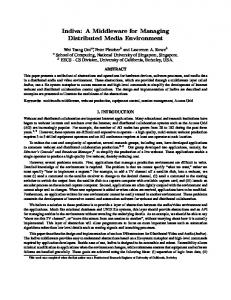
The main idea of the proposed algorithm is to extract the desired lesion from the 3D volume data using Bayesian-rule based 3D region growing starting from multiple seeds specified by the user. The algorithm is based on the assumption that the intensity distribution of the lesion can be modeled as Gaussian distri-

butions. Figure 1 shows the intensity distribution of the normal liver region and the tumorous region of one of the patient data sets. To cope with the variance of tumors, we employ a bag of Gaussians, which is however different from existing works where the tumor is modeled by a single Gaussian.

5000

tumor liver

4500

4000

No. of voxels

3500

3000

2500

2000

1500

1000

500

0 1000

1020

1040

1060

1080

1100

1120

1140

Density of CT image

Fig. 1. Example intensity distributions of liver and lesion.

Figure 2 summarizes the proposed algorithm which includes three stages. In the first stage, the input images are preprocessed with smoothing and noise removal. In the second stage, the proposed 3D region growing algorithm is applied. The third stage is post-processing which includes morphological operations such as hole removal. Details will be discussed in the following sections.

2.1

Region Growing

Region growing algorithm is used to look for similar voxels as the seeds provided by users. The seeds belong to two classes. One class is normal liver, and the other is lesion. The Bayesian rule-based region growing works as a classifier to classify the voxels into these two classes. Given two classes of voxels, the normal liver ω1 and the lesion ω2 , their prior probabilities are denoted as P (ωj ), and their class-conditional probability density function is p(I|ωj ), j = 1, 2, respectively, where I is the data in the feature space. The posterior probability of I is given by P (ωj |I) =

p(I|ωj )P (ωj ) , j = 1, 2, p(I)

(1)

3D CT data

Pre-processing

3D Region Growing

Combine similar Gaussian models of tumor

Compute initial Gaussian Models G and Gi l

t

Gt' i Get a new voxel X connecting with the current region

Yes Post processing

Converged?

Update

Include X into the current region Yes

No Tumor region segmented

Compute local PDF at X

Gt' i

Both criteria fufilled 'i w.r.t. Gt ? No Give up X

Fig. 2. Flowchart of the proposed algorithm.

with evidence p(I) given by p(I) =

2 X

p(I|ωj )P (ωj ).

(2)

j=1

The Bayesian decision rule for minimizing the probability of error is [7]: Decide I ∈ ω1 if P (ω1 , I) > P (ω2 , I); otherwise decide I ∈ ω2 .

(3)

Substituting Equations 1 and 2 into Equation 3, we obtain an equivalent rule in the terms of class-conditional probability density functions: Decide I ∈ ω1 if p(I|ω1 )P (ω1 ) > p(I|ω2 )P (ω2 ); otherwise decide I ∈ ω2 . (4) Specially, if P (ω1 ) = P (ω2 ), then Decide I ∈ ω1 if p(I|ω1 ) > p(I|ω2 ); otherwise decide I ∈ ω2 .

(5)

In this case, it is assumed that the normal liver class and the lesion class have the same priors. Therefore, the Bayesian rule is applied in form of Equation 5. As mentioned before, the intensity, denoted as x, of the voxel are considered as the feature of the point. The class-conditional probability density function (PDF) of the liver and lesion are estimated beforehand and assumed as two Gaussians with parameter µj , σj ,j = 1, 2, being the mean and the variance, respectively: 1 1 exp(− (x − µj )2 /σj2 ), p(x|ωj ) = √ 2 2πσj

(6)

Decide x ∈ ω1 if p(x|ω1 ) > p(x|ω2 ); otherwise decide x ∈ ω2 .

(7)

In this case,

Based on the above theory, the region growing algorithm is used to classify voxels into two classes: liver and lesion. The liver class is modeled by a single Gaussian, whereas the tumor class is modeled by multiple Gaussians. More specifically, the algorithm starts by specifying several seed points. One of the seeds Sl should be located inside the liver region. And at least one seed St1 , ..., Stn (n > 0) should be located inside the lesion. For inhomogeneous lesion, it is suggested to choose more seeds scattered inside the lesion. Furthermore, the seeds should be chosen away from the edges between lesion and liver. Then these seeds are used to set up initial configurations. Define a neighborhood of a voxel in 3D is a 5 × 5 × 5 cube centered at it. It is assumed that the neighborhood of each seed is inside the liver or the lesion. First, the parameters {µl , σl } of Gaussian model Gl are estimated using all the 11 × 11 × 11 neighboring voxels of the liver seed point as samples. Second, for each seed point in

the lesion, Git {µit , σti } are also estimated. Gjt and Gkt are considered as similar, if |µjt − µkt | is less than a predefined Gaussian combination threshold Tc . Then all the similar Gaussians of the lesion are combined by calculating new values of ′i ′i parameter G′i t {µt , σt }(i = 1, ..., m). With initial Gaussian models of liver and lesion obtained from previous step, the 3D region growing algorithm is performed starting from the seed points. It adds neighboring voxels one at a time into the regions if they have similar properties with respect to the predefined criteria. Here two criteria are used to measure the similarity. 1. The intensity of the voxel should be accepted by one of the Gaussians of the lesion G′i t . Equation 7 is used to make the decision. 2. One of the intensity distribution models of lesions and that of the current voxel should be similar. The intensity distribution of a specific point in the 3D image is estimated by the intensity histogram within its 3D neighborhood. Assume the histogram is hi (x), and histogram of current point is h′ (x). Here, the Bhattacharyya distance [8] is used to measure the similarity. BC(hi , h′ ) =

Xp hi (x)h′ (x).

(8)

x

It is always between 0 and 1, 1 indicating the strongest similarity between the histograms, 0 the weakest. In the implementation, a predefined threshold Td is used to discard distinguish voxels. Voxels which meet both criteria are considered as a part of the lesion and added into the region. Their intensity values are also used to update the pa′i ′i rameters of the corresponding Gaussian model G′i t {µt , σt }. The region growing algorithm will examine all the connected voxels one by one until the region fixes. 2.2

Pre-processing

Before applying region growing algorithm, the CT images are smoothed in order to reduce some noise. There are always some noise all over the CT images, especially when the spacing is very small. The image filter, “CurvatureAnisotropicDiffusionImageFilter”, which is implemented by ITK [9], is used. The purpose of this filter is to smooth the image but preserve the edges at the same time such that the regions of lesions won’t be damaged because of smoothing. 2.3

Post-processing

Although smoothing has already been applied on the input CT images, there are still some noise voxels whose intensity is quite different from the desired lesion. Therefore, volumes obtained by region growing may have some small holes inside it. Morphological operations are performed on the volumes to remove them.

3

Experiments and Results

The program was developed in C++ using ITK [9]. It was executed to segment the lesions one at a time. It requires several inputs, such as a set of CT scans, coordinates of the seed points, Gaussian combination threshold Tc , and Bhattacharyya distance threshold Td . As mentioned before, the seeds in the lesion should be scattered. They are usually chosen by examining whether their intensities are representative of all the voxels in the lesion. Usually five to six seeds are chosend for the large and inhomogeneous tumor. Tc is set by experience. If the lesion region is relatively homogeneous, only one Gaussian model will be used, and thus Tc is set to a large number. When multiple Gaussians are used, the range of intensity variation inside the lesion has to be estimated, and Tc is set to a small number according to the range. In only a few cases in this experiment, two or three Gaussians are used and Tc is set to around 3. Td whose value is in the range of 0 to 1 is usually set by experiment. If the segmentation result has serious leakage problems, the threshold should be set to a larger number. On the other hand, if the region has not grown widely enough, the threshold should be set to a smaller number. The proposed algorithm has been trained on CT images of four patients with ten tumors in the training data, and evaluated on CT images of six patients with ten tumors in testing data. Figure 3 shows the segmented lesion boundaries for a selection of slices of different patients in the training data, compared with segmentation reference. The segmentation results of the testing data were compared to manual expert segmentation and given a score for each case. The scale was set such that a score of 100 points was awarded to a perfect tumor segmentation with 100% volume overlap with the expert segmentation. Table 1 shows the evaluation results of the testing data. The algorithm provided reasonable results of most of the lesions. In some cases like IMG08 L1 and IMG09 L1 in Table 1, the algorithm may fail. It is probably because the region will leak when the boundary is very blur. Therefore, the leakage would be constrained if we can delineate the tumor region in some way. Another possible reason is the algorithm highly depends on the choice of seed points and thresholds. However, it is not easy to choose robust values. The values are usually chosen by several experiment and experience. The program was run on a MacPro with two 2GHz Dual-Core Intel Xeon and 4GB 667MHz DDR2 memory. The running time was about ten to thirty minutes for all the lesions. For some small lesions, it was pretty fast (less than 10 minutes). However, it took a longer time to segment the extremely large tumor like IMG07 L1 and IMG08 L1 in the testing data. It should be noted that we made no attempt to tune the algorithm’s parameters to reduce the execution time. Instead, as these parameters are only set once in the beginning of the 3D segmentation and no manual intervention is added during automatic growing (to inspect the performance), the primary concern is the convergence of growing. Thus there could be a great potential to increase execution speed.

(a)

(b)

(c)

(d)

Fig. 3. Segmentation references (top row) and results (bottom row) of training data set. (a) Lesion 2 from Patient 1. (b) Lesion 3 from Patient 2. (c) Lesion 1 from Patient 3. (d) Lesion 4 from Patient 4.

4

Discussion and Conclusion

In this work, we have presented a semi-automatic algorithm to segment liver tumors from computed tomography (CT) images. To cope with the variance of tumors, we model liver tumor using a bag of Gaussians, and employ a 3D seeded region growing method. The bag of Gaussians are initialized at manually selected seeds and updated during growing process iteratively. Two criteria are fulfilled for the growing: one is the Bayesian decision rule, and the other is a model matching measure. Finally, morphological operations are performed to refine the results. By exploring the segmentation and evaluation results, the pros and cons of the proposed algorithm can be concluded as follows. First, as shown in Figure 3, the algorithm provides reasonable results for most of the lesions, especially when the intensity difference between tumor and normal liver is large. Second, the region will grow in 3D. Thus, the user only need to pick seed points once, and do not need to initialize the algorithm for every slice. It involves very little manual (and simple) operation in initial seed selection. There is no other constraint or further manual work during the growing. Also the continuity of the segmented object in 3D is better than that of 2D-based segmentation algorithms (Figure 4). On the other hand, the region growing process is not easy to control in 3D when the boundaries are unclear. It has a very high probability to leak, and the leakage will propagate to adjacent slices. The proposed algorithms will detect the top and bottom slices of the tumor automatically. However, in some

Table 1. Results of the comparison metrics and scores for all the testing data. S: score. T: total score.

Tumor IMG05 L1 IMG05 L2 IMG05 L3 IMG06 L1 IMG06 L2 IMG07 L1 IMG07 L2 IMG08 L1 IMG09 L1 IMG10 L1 Average

Overlap Error (%) S 42.47 67 37.21 71 47.21 64 59.58 54 67.56 48 24.70 81 35.95 72 28.39 78 57.20 56 20.75 84 42.10 68

(a)

Volume Difference (%) S 32.60 66 13.68 86 26.12 73 118.54 0 2.24 98 11.72 88 53.70 44 29.32 70 133.39 0 8.81 91 43.01 62

Ave. Surf Dist. (mm) S 3.27 17 1.35 66 2.05 48 2.55 36 2.04 49 3.02 24 2.18 45 6.55 0 3.41 14 1.20 70 2.76 37

RMS Surf. Dist. (mm) S 4.45 38 1.77 75 2.76 61 3.28 54 2.43 66 4.31 40 2.84 60 11.99 0 3.95 45 1.58 78 3.94 52

Max. Surf. Dist. (mm) S 14.78 63 4.86 88 9.44 76 8.71 78 6.70 83 25.71 36 13.65 66 60.51 0 12.75 68 12.18 70 16.93 63

T 50 77 64 44 69 54 58 30 36 78 56

(b)

Fig. 4. Snapshots of 3D segmented tumors after smoothing. (a) Lesion 2 from Patient 1. (b) Lesion 4 from Patient 4.

complicated cases, the algorithm cannot handle very well, such that there will be more segmentation errors in top and bottom slices. The main problem with the proposed algorithm is the leakage problem. In order to control the region growing more effectively, shape constraints and prior knowledge may be helpful. However, how to embed such constraints into the region growing in 3D dynamically will become another difficult issue.

Acknowledgments This work is supported by a research grant (SBIC RP C-008/2006) from the Singapore BioImaging Consortium, Agency for Science, Technology and Research.

References 1. Chen, Y., Yi, Q., Mao, Y.: Cluster of liver cancer and immigration: A geographic analysis of incidence data for ontario 1998-2002. International Journal of Health Geographics 7(28) (2008) 2. Seo, K.: Automatic hepatic tumor segmentation using composite hypotheses. Image Analysis and Recognition 3656 (2005) 922 – 929 3. Yim, P., Foran, D.: Volumetry of hepatic metastases in computed tomography using the watershed and active contour algorithms. In: Proceedings of the 16th IEEE Symposium on Computer-based Medical Systems. (2003) 329 – 335 4. Lu, R., Marziliano, P., Thng, C.: Liver tumor volume estimation by semi-automatic segmentation method. In: Proceedings of the 27th Annual Conference of IEEE Engineering in Medicine and Biology. (2005) 3296 – 3299 5. Zhao, B., Schwartz, L., Jiang, L., Colville, J., Moskowitz, C., Wang, L., Leftowitz, R., Liu, F., Kalaigian, J.: Shape-constraint region growing for delineation of hepatic metastases on contrast-enhanced computed tomograph scans. Investigative Radiology 41(10) (2006) 753 – 762 6. Deng, X., Du, G.: 3D Liver Tumor Segmentation Challenge 2008, http://lts08.bigr.nl/index.php. (2008) 7. Duda, R.O., Hart, P.E., Stork, D.G.: Pattern Classification. second edn. A WileyInterscience Publication. John Wiley and Sons (2001) 8. Bhattacharyya, A.: On a measure of divergence between two statistical populations defined by probability distributions. Bull. Calcutta Math. Soc. 35 (1943) 99 – 109 9. Ibanez, L., Schroeder, W., Ng, L., Cates, J.: The ITK Software Guide. Kitware, Inc. ISBN 1-930934-15-7, http://www.itk.org/ItkSoftwareGuide.pdf. Second edn. (2005)