Semi-empirical dissipation source functions for ocean waves: Part I ...

Generated using V3.0 of the official AMS LATEX template–journal page layout FOR AUTHOR USE ONLY, NOT FOR SUBMISSION!

Semi-empirical dissipation source functions for ocean waves: Part I, definition, calibration and validation. Fabrice Ardhuin ∗, Jean-Franc ¸ ois Filipot and Rudy Magne Service Hydrographique et Oc´ eanographique de la Marine, Brest, France

arXiv:0907.4240v3 [physics.ao-ph] 2 Jan 2010

Erick Rogers Oceanography Division, Naval Research Laboratory, Stennis Space Center, MS, USA

Alexander Babanin Swinburne University, Hawthorn, VA, Australia

Pierre Queffeulou Ifremer, Laboratoire d’Oc´ eanographie Spatiale, Plouzan´ e, France

Lotfi Aouf and Jean-Michel Lefevre UMR GAME, M´ et´ eo-France - CNRS, Toulouse, France

Aron Roland Technological University of Darmstadt, Germany

Andre van der Westhuysen Deltares, Delft, The Netherlands

Fabrice Collard CLS, Division Radar, Plouzan´ e, France

ABSTRACT New parameterizations for the spectral dissipation of wind-generated waves are proposed. The rates of dissipation have no predetermined spectral shapes and are functions of the wave spectrum, in a way consistent with observation of wave breaking and swell dissipation properties. Namely, swell dissipation is nonlinear and proportional to the swell steepness, and wave breaking only affects spectral components such that the non-dimensional spectrum exceeds the threshold at which waves are observed to start breaking. An additional source of short wave dissipation due to long wave breaking is introduced, together with a reduction of wind-wave generation term for short waves, otherwise taken from Janssen (J. Phys. Oceanogr. 1991). These parameterizations are combined and calibrated with the Discrete Interaction Approximation of Hasselmann et al. (J. Phys. Oceangr. 1985) for the nonlinear interactions. Parameters are adjusted to reproduce observed shapes of directional wave spectra, and the variability of spectral moments with wind speed and wave height. The wave energy balance is verified in a wide range of conditions and scales, from the global ocean to coastal settings. Wave height, peak and mean periods, and spectral data are validated using in situ and remote sensing data. Some systematic defects are still present, but the parameterizations probably yield the most accurate overall estimate of wave parameters to date. Perspectives for further improvement are also given.

sities of the surface elevation variance F distributed over frequencies f and directions θ can be put in the form

1. Introduction a. On phase-averaged models

dF (f, θ) = Satm (f, θ)+Snl (f, θ)+Soc (f, θ)+Sbt (f, θ), (1) dt

Spectral wave modelling has been performed for the last 50 years, using the wave energy balance equation (Gelci et al. 1957). This model for the evolution of spectral den-

1

where the Lagrangian derivative is the rate of change of the spectral density when following a wave packet at its group speed in physical and spectral space. This spectral advection particularly includes changes in direction due to the Earth sphericity and refraction over varying topography (e.g. Munk and Traylor 1947; Magne et al. 2007) and currents, and changes in wavelength or period in similar conditions (Barber 1949). The source functions on the right hand side are separated into an atmospheric source function Satm , a nonlinear scattering term Snl , an ocean source Soc , and a bottom source Sbt . This separation, like any other, is largely arbitrary. For example, waves that break are highly nonlinear and thus the effect of breaking waves that is contained in Soc is intrisically related to the non-linear evolution term contained in Snl . Yet, compared to the usual separation of deep-water evolution into wind input, non-linear interactions, and dissipation, it has the benefit of identifying where the energy and momentum is going to or coming from, which is a necessary feature when ocean waves are used to drive or are coupled with atmospheric or ocean circulation models (e.g. Janssen et al. 2004; Ardhuin et al. 2008b). Satm , which gives the flux of energy from the atmospheric non-wave motion to the wave motion, is the sum of a wave generation term Sin and a wind generation term Sout (often referred to as “negative wind input”, i.e. a wind output). The nonlinear scattering term Snl represents all processes that lead to an exchange of wave energy and momentum between the different spectral components. In deep and intermediate water depth, this is dominated by cubic interactions between quadruplets of wave trains, while quadratic nonlinearities play an important role in shallow water (e.g. WISE Group 2007). The ocean source Soc may accomodate wave-current interactions1 and interactions of surface and internal waves, but it will be here restricted to wave breaking and wave-turbulence interactions. The basic principle underlying equation (1) is that waves essentially propagate as a superposition of almost linear wave groups that evolve on longer time scales as a result of weak-in-the-mean processes (e.g. Komen et al. 1994). Recent reviews have questioned the possibility of further improving numerical wave models without changing this basic principle (Cavaleri 2006). Although this may be true in the long term, we demonstrate here that it is possible to improve model results significantly by including more physical features in the source term parameterizations. The main advance proposed in the present paper is the adjustment of a shape-free dissipation function based on today’s em-

pirical knowledge on the breaking of random waves (Banner et al. 2000; Babanin et al. 2001) and the dissipation of swells over long distances (Ardhuin et al. 2009b). The present formulations are still semi-empirical, in the sense that they are not based on a detailed physical model of dissipation processes, but they demonstrate that progress is possible. This effort opens the way for completely physical parameterizations (e.g. Filipot et al. 2010) that will eventually provide new applications for wave models, such as the estimation of statistical parameters for breaking waves, including whitecap coverage and foam thickness. Other efforts, less empirical in nature, are also under way to arrive at better parameterizations (e.g. Banner and Morison 2006; Babanin et al. 2007; Tsagareli 2008), but they yet have to produce a practical alternative for wave forecasting and hindcasting. b. Shortcomings of existing parameterizations

All wave dissipation parameterizations up to the work of van der Westhuysen et al. (2007) had no quantitative relationship with observed features of wave dissipation, and the parameterizations were generally used as set of tuning knobs to close the wave energy balance. The parameterization of the form proposed by Komen et al. (1984) have produced a family loosely justified by the so-called ‘random pulse’ theory of (Hasselmann 1974). These take a generic form "  2 # k k 0.5 4.5 4 , (2) Soc (f, θ) = Cds g kr Hs δ1 + δ2 kr kr in which Cds is a negative constant, and kr is an energyweighted mean wavenumber defined from the entire spectrum, and Hs is the significant wave height. In the early and latest parameterizations, the following definition was used #1/r " Z Z 16 fmax 2π r k E (f, θ) df dθ , (3) kr = Hs2 0 0 where r is a chosen real constant, typically r = −0.5 or r = 0.5. These parameterizations are still widely used in spite of inconsistencies in the underlying theory. Indeed, if whitecaps do act as random pressure pulses, their average work on the underlying waves only occurs because of a phase correlation between the vertical orbital velocity field and the moving whitecap position, which travels with the breaking wave. In reality the horizontal shear is likely the dominant mechanism (Longuet-Higgins and Turner 1974), but the question of correlation remains the same. For any given whitecap, such a correlation cannot exist for all spectral wave components: a whitecap that travels with one wave leads to the dissipation of spectral wave components that

1 In the presence of variable current, the source of energy for the wave field, i.e. the work of the radiation stresses, is generally hidden when the energy balance is written as an action balance (e.g. Komen et al. 1994).

2

An alternative and widely used formulation has been proposed by Tolman and Chalikov (1996), and some of its features are worth noting. It combines two distinct dissipation formulations for high and low frequencies, with a transition at two times the wind sea peak frequency. Whereas Janssen et al. (1994) introduced the use of two terms, k and k 2 in eq. (2), in order to match the very different balances in high and low frequency parts of the spectrum, they still had a common fixed coefficient, Cds g 0.5 kr4.5 Hs4 . In Tolman and Chalikov (1996) these two dissipation terms are completely distinct, the low frequency part being linear in the spectrum and proportional to wind friction velocity u⋆ , the high frequency part is also linear and proportional to u2⋆ . In this formulation the frequency dependence of the two terms is also prescribed. Tolman and Chalikov (1996) further included swell attenuation by the wind, based on numerical simulations of the airflow above waves (Chalikov and Belevich 1993), here noted Sout . At relatively short fetches, these source terms are typically a factor 2 to 3 smaller than those of Janssen et al. (1994), which was found to produce important biases in wave growth and wave directions at short fetch (Ardhuin et al. 2007). Another set of parameterizations was proposed by Makin and Stam (2003). It is appropriate for high winds conditions but does not produce accurate results in moderate sea states (Lef`evre et al. 2004). Finally, among the many formulations proposed we may cite one by Polnikov and Inocentini (2008), but its accuracy appears generally less than with the model presented here, in particular for mean periods. Based on observations of large wave height gradients in rapidly varying currents, Phillips (1984) proposed a dissipation rate proportional to the non-dimensional spectrum B, also termed ’saturation spectrum’. Banner et al. (2000) indeed found a correlation between the breaking probability of dominant waves and the saturation, when the latter is integrated over a finite frequency bandwidth and all directions., with breaking occuring when B exceeds a threshold Br . Alves and Banner (2003) proposed to define the dissipation Soc by B/Br to some power, multiplied by a Komentype dissipation term. Although this approach avoided the investigation of the dissipation of non-breaking waves, it imported all the above mentionned defects of that parameterization. Further, these authors used a value for Br that is much higher than suggested by observations, which tends to disconnect the parameterization from the observed effects (Babanin and van der Westhuysen 2008). The use of a saturation parameter was taken up again by van der Westhuysen et al. (2007), hereinafter WZB, who, Like Alves and Banner (2003), integrated the saturation spectrum over directions, giving Z 2π k 3 F (f, θ′ )Cg /(2π)dθ′ . (5) B (f ) =

propagate in similar directions, with comparable phase velocities. However, whitecaps moving in one direction will give (on average) a zero correlation for waves propagating in the opposite direction because the position of the crests of these opposing waves are completely random with respect to the whitecap position. As a result, not all wave components are dissipated by a given whitecap (others should even be generated), and the dissipation function cannot take the spectral form given by Komen et al. (1984). A strict interpretation of the pressure pulse model gives a zero dissipation for swells in the open ocean because the swell wave phases are uncorrelated to those of the shorter breaking waves. There is only a negligible dissipation due to short wave modulations by swells and preferential breaking on the swell crests (Phillips 1963; Hasselmann 1971; Ardhuin and Jenkins 2005). Still, the Komen et al. (1984) type dissipation terms are applied to the entire spectrum, including swells, without any physical justification. In spite of its successful use for the estimation of the significant wave height Hs and peak period Tp , these fixedshape dissipation functions, from Komen et al. (1984) up to Bidlot et al. (2007a), have built-in defects. Most conspicuous is the spurious amplification of wind sea growth in the presence of swell (e.g. van Vledder and Hurdle 2002), which is contrary to all observations (Dobson et al. 1989; Violante-Carvalho et al. 2004; Ardhuin et al. 2007). Associated wih that defect also comes an underestimation of the energy level in the inertial range, making these wave models ill-suited for remote sensing applications, as will be exposed below. Also, these parameterizations typically give a decreasing dissipation of swell with increasing swell steepness, contrary to all observations from Darbyshire (1958) to Ardhuin et al. (2009b). This effect is easily seen by taking a sea state composed of a swell and wind sea of energy E1 and E2 and mean wavenumbers k1 and k2 , respectively, with k2 > k1 . The overall mean wavenumber is kr = [(k1r E1 + k2r E2 ) /(E1 + E2 )]

1/r

.

(4)

Equation (2) gives a dissipation that is proportional to kr3.5 (E1 + E2 ) in the low frequency limit. Now, if we keep k1 , k2 an E2 constant and only increase the swell energy E1 , the relative change in dissipation is, according to (2), proportional to x = 3.5[(k1 /kr )r −1]/r+2. For r = 0.5, as used by (Bidlot et al. 2005, hereinafter BAJ), and k1 /kr < 0.51, x is negative (i.e. the dissipation decreases with increasing swell energy). For equal energy in sea and swell, this occurs when k1 /k2 < 0.3, which is generally the case with sea and swell in the ocean. This erroneous decrease of swell dissipation with increasing swell steepness is reduced when the model frequency range is limited to maximum frequency of 0.4 Hz, in which case the lowest winds (less than 5 m/s) are unable to produce a realistic wind sea level, hence limiting the value of kr to relatively small values.

0

3

From this, they defined the source function  p/2 p B(f ) Soc,WZB (f, θ) = −C gk , Br

rameterizations at all scales, in order to provide a robust and comprehensive parameterization of wave dissipation. (6)

c. A new set of parameterizations and adjustments to get adequate balances

where C is a positive constant, Br is a constant saturation threshold and and p is a coefficient that varies both with the wind friction velocity u⋆ and the degree of saturation B(f )/Br with, in particular, p ≈ 0 for B(f ) < 0.8Br . For non breaking waves, when p ≈ 0, the dissipation is too large by at least one order of magnitude, making the parameterization unfit for oceanic scale applications with wave heights in the Atlantic underpredicted by about 50% (Ardhuin and Le Boyer 2006). In van der Westhuysen (2007) this was addressed by reverting back to Komen et al. (1984) dissipation for non-breaking waves, but no solution for the dissipation of these spectral components was proposed. In WZB, the increase of p with the inverse wave age u⋆ /C was designed to increase Soc at high frequency, which was needed to obtain a balance with the Satm term in equation (1). This indicates that, besides the value of the saturation Br , other factors may be important, such as the directionality of the waves (Banner et al. 2002). Other observations clearly show that the breaking rate of high frequency waves is much higher for a given value of B, probably due to cumulative effects by which the longer waves are modifying the dissipation of shorter waves. Banner et al. (1989) and Melville et al. (2002) have shown how breaking waves suppress the short waves on the surface, and we will show here that a simple estimation of the dominant breaking rates based on the observations by Banner et al. (2000) suggests that this effect is dominant for wave frequencies above three times the windsea peak frequency. Young and Babanin (2006) arrived at the same conclusion from the examination of wave spectra, and proposed a parameterization for Soc that included a new term, the cumulative term, to represent theis effect. Yet, their estimate was derived for very strong wind-forcing conditions only. Further, their interpretation of the differences in parts of a wave record with breaking and non-breaking waves implies an underestimation of the dissipation rates because the breaking waves have already lost some energy when they are observed and the non-breaking waves are not going to break right after they have been observed. Also, since the spectra are different, nonlinear interactions must be different, even on this relatively small time scale (e.g. Young and van Vledder 1993, figure 5), and the differences in spectra may not be the result of dissipation alone. Finally, the recent measurement of swell dissipation by Ardhuin et al. (2009a) has revealed that the dissipation of non-breaking waves is essentially a function of the wave steepness, and a very important process for ocean basins larger than 1000 km. Because of the differences between coastal and larger scale sea states (e.g. Long and Resio 2007), it is paramount to verify the source function pa-

It is thus time to combine the existing knowledge on the dissipation of breaking and non-breaking waves to provide an improved parameterization for the dissipation of waves. Our objective is to provide a robust parameterization that improves existing wave models. For this we will use the parameterization by BAJ as a benchmark, because it was shown to provide the best forecasts on global scales (Bidlot et al. 2007b) before the advent of the parameterizations presented here. BAJ is also fairly close to the widely used “WAM-Cycle 4” parameterization by Janssen and others (Komen et al. 1994). We will first present a general form of the dissipation terms based on observed wave dissipation features. The degrees of freedom in the parameterization are then used to adjust the model result. In particular we adujst a cumulative breaking effect and a wind sheltering effect that, respectively, dissipates and reduces the wind input to short waves as a function of longer waves characteristics. A comprehensive validation of wave parameters is then presented using field experiments and a one year hindcast of waves at the global and regional scale, in which all possible wave measurements are considered, with significant wave heights ranging from 0 to 17 m. The model is further validated with independent data at regional and global scales. Tests and verification in the presence of currents, and using a more realistic parameterizations of wave-wave interactions will be presented in parts II and III. These may also include some replacement of the arbitrary choices made here in the details of the dissipation parameters, with physicallymotivated expressions. 2. Parameterizations Several results will be presented, obtained by a numerical integration of the energy balance. Because numerical choices can have important effects (e.g. Tolman 1992; Hargreaves and Annan 2000), a few details should be given. All calculations are performed with the WAVEWATCH IIITM modelling framework (Tolman 2008, 2009), hereinafter WWATCH, using the third order spatial and spectral advection scheme, and including modifications of the source terms described here. In all cases ran with WWATCH, the source terms are integrated with the fully implicit scheme of Hargreaves and Annan (2000), combined with the adaptative time step and limiter method of Tolman (2002a), in which a minimum time step of 10 s is used, so that the limiter on wind-wave growth is almost never activated. The diagnostic tail, proportional to f −5

4

A few tests have indicated that a threshold Rec = 2 × 105 m/Hs provides reasonable result, although it may be a also be a function of the wind speed, and we have no explanation for the dependence on Hs . A constant threshold close to 2 × 105 provides similar results. Here we shall use Cdsv = 1.2, but the results are not too sensitive to the exact value. The parameterization of the turbulent boundary layer is more problematic. Without direct measurements in the boundary layer, there is ample room for speculations. From the analogy with an oscillatory boundary layer over a fixed bottom (Jensen et al. 1989), the values of fe inferred from the swell observations, in the range 0.004 to 0.013 (Ardhuin et al. 2009b), correspond to a surface with a very small roughness. Because, we also expect the wind to influence fe , the parameterization form includes adjustable effects of wind speed on the roughness, and an explicit correction of fe . This latter correction takes the form of a Taylor expansion to first order in u⋆ /uorb ,   u⋆ , (10) fe = s1 fe,GM + [|s3 | + s2 cos(θ − θu )] uorb

is only imposed at a cut-off frequency fc set to fc = fFM fm .

(7)

Here we take fFM = 10 and define the mean frequency as fm =1/Tm0,1 . Hence fc is generally above the maximum model frequency that we fixed at 0.72 Hz, and the high frequency tail is left to evolve freely. Some comparison tests are also done with other parameterizations using a lower value of fc , typically set at 2.5 fm (Bidlot et al. 2007a). In such calculations, although the net source term may be non-zero at frequencies above fc , there is no spectral evolution due to the imposed tail. a. Nonlinear wave wave interactions

All the results discussed and presented in this section are obtained with the Discrete Interaction Approximation of Hasselmann et al. (1985). The coupling coefficient that gives the magnitude of the interactions is Cnl . Based on comparisons with exact calculations, Komen et al. (1984) adjusted the value of Cnl to 2.78 × 107 , which is the value used by Bidlot et al. (2005). Here this constant will be allowed to vary slightly. This parameterization is well known for its shortcomings (Banner and Young 1994), and the adjustment of other parameters probably compensates for some of these errors. This matter will be fully discussed in Part III.

where fe,GM is the friction factor given by Grant and Madsen’s (1979) theory for rough oscillatory boundary layers without a mean flow. Adequate swell dissipation is obtained with constant values of fe in the range 0.004 to 0.007, but these do not necessarily produce the best results when comparing wave heights to observations. Based on the simple idea that most of the air-sea momentum flux is supported by the pressure-slope correlations that give rise to the wave field (Donelan 1998; Peirson and Banner 2003), we have set the surface roughness to

b. Swell dissipation

Observations of swell dissipation are consistent with the effect of friction at the air-sea interface (Ardhuin et al. 2009a), resulting in a flux of momentum from the wave field to the wind (Harris 1966). We thus write the swell dissipation as a negative contribution Sout which is added to Sin to make the wind-wave source term Satm . Using the method of Collard et al. (2009), a systematic analysis of swell observations by Ardhuin et al. (2009a) showed that the swell dissipation is non-linear, possibly related to a laminar-to-turbulent transition of the oscillatory boundary layer over swells. Defining the boundary Reynolds number Re= 4uorb aorb /νa , where uorb and aorb are the significant surface orbital velocity and displacement amplitudes, and νa is the air viscosity, we take, for Re less than a critical value Rec o ρa n √ (8) 2k 2νσ F (f, θ) , Sout (f, θ) = −Cdsv ρw

z0′ = rz0 z0

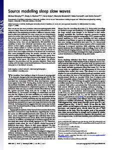
where rz0 is here set to 0.04, of the roughness for the wind. We thus give the more generic equation (10) for fe , with fe,GM of the order of 0.003 for values of aorb /z0′ of the order of 2×105 . The coefficients s2 and s3 of the O(u⋆ /uorb ) correction have been adjusted to -0.018 and 0.015, respectively, the former negative value giving a stronger dissipation for swells opposed to winds, when cos(θ − θu ) < 0. This gives a range of values of fe consistent with the observations, and reasonable hindcasts of swell decay (Fig. 1), with a small underestimation of dissipation for steep swells. An increase of s1 from 0.8 to 1.1 produces negative biases on Hs of the order of 30% at all oceanic buoys (40% for a partial wave height estimated from a spectrum restricted to periods around 15 s), so that the magnitude of the swell dissipation cannot be much larger than chosen here. Further discussion and validation of the swell dissipation is provided by the global scale hindcasts in Section 4.

where the constant Cdsv is equal to 1 in Dore (1978)’s laminar theory. When the boundary layer is expected to be turbulent, for Re≥Rec , we take Sout (f, θ) = −

ρa  16fe σ 2 uorb /g F (f, θ) . ρw

(11)

(9)

5

estimating a breaking probability. We started from the simplest possible dissipation term formulated in terms of the direction-integrated spectral saturation B (f ) given by eq. (5), with a realistic threshold B0r = 1.2×10−3 corresponding to the onset of wave breaking (Babanin and Young 2005). This saturation parameter corresponds exactly to the α parameter defined by Phillips (1958). The value B0 = 8 × 10−3 , given by Phillips, corresponds to a self-similar sea state in which waves of all scales have the same shape, limited by the breaking limit. This view of the sea state, however, ignores completely wave directionality. Early tests of parameterizations based on this definition of B indicated that the spectra were too narrow (Ardhuin and Le Boyer 2006). This effect could be due to many errors. Because Banner et al. (2002) introduced a directional width in their saturation to explain some of the variability in observed breaking probabilities, we similarly modify the definition of B. Expecting also to have different dissipation rates in different directions, we define a saturation B ′ that would correspond, in deep water, to a normalized velocity variance projected in one direction (in the case sB = 2), with a further restriction of the integration of directions controlled by ∆θ , Fig. 1. Comparison of modelled swell significant heights, following the propagation of the two swells shown by Ardhuin et al. (2009) with peak periods of 15 s and high and low dissipation rates. Known biases in the level 2 data have been corrected following Collard et al. (2009).

B ′ (f, θ) =

Z

θ+∆θ θ−∆θ

k 3 cossB (θ − θ′ ) F (f, θ′ )

Cg ′ dθ , 2π

(12)

Here we shall always use ∆θ = 80◦ . As a result, a sea state with two systems of same energy but opposite direction will typically produce much less dissipation than a sea state with all the energy radiated in the same direction. We finally define our dissipation term as the sum of the saturation-based term of Ardhuin et al. (2008a) and a cumulative breaking term Sbk,cu , h C sat 2 Soc (f, θ) = σ Bds2 δd max {B (f ) − Br , 0} r i 2 + (1 − δd ) max {B ′ (f, θ) − Br , 0} F (f, θ)

c. Wave breaking

Observations show that waves break when the orbital velocity at their crest Uc comes close to the phase speed C, with a ratio Uc /C > 0.8 for random waves (Tulin and Landrini 2001; Stansell and MacFarlane 2002; Wu and Nepf 2002). It is nevertheless difficult to parameterize the breaking of random waves, since the only available quantity here is the spectral density. This density can be related to the orbital velocity variance in a narrow frequency band. This question is addressed in detail by Filipot et al. (2010). Yet, a proper threshold has to be defined for this quantity, and the spectral rate of energy loss associated to breaking has to be defined. Also, breaking is intricately related to the complex non-linear evolution of the waves (e.g. Banner and Peirson 2007). These difficulties will be ignored here. We shall parameterize the spectral dissipation rate directly from the wave spectrum, in a way similar to WZB. Essentially we distiguish between spontaneous and induced breaking, the latter being caused by large scale breakers overtaking shorter waves, and causing them to be dissipated. For the spontaneous breaking we parameterize the dissipation rate directly from the spectrum, without the intermediate step of

+

Sbk,cu (f, θ) + Sturb (f, θ).

(13)

where B (f ) = max {B ′ (f, θ), θ ∈ [0, 2π[} .

(14)

The combination of an isotropic part (the term that multiplies δd ) and a direction-dependent part (the term with 1 − δd ) was intended to allow some control of the directional spread in resulting spectra. This aspect is illustrated in figure 2 with a hindcast of the November 3 1999 case during the Shoaling Waves Experiment (Ardhuin et al. 2007). Clearly, the isotropic saturation in the TEST442 dissipation (with the original threshold Br = 0.0012) produces very narrow spectra, even though it is known that the DIA parameterization for nonlinear interactions, used here, tends to broaden the spectra. The same behaviour is obtained with the isotropic parameterization by van der 6

(a)

f (Hz)

(b)

Ccu=−1, su=0 Ccu=−0.4, su=1 2 Ccu=−0.4, su=1 = 1, Br = 0.0012 3 Ccu=−0.4, su=1 = 0, Br = 0.0009

(c)

Fig. 2. Wave spectra on 3 November 1999 at buoy X3 (fetch 39 km, wind speed U10 = 9.4 m s−1 ), averaged over the time window 1200-1700 EST, from observations and model runs, with different model parameterizations (symbols): BAJ stands for Bidlot et al. (2005). (a) Energy, (b) mean direction (c) directional spread. This figure is analogue to the figures 10 and 11 in Ardhuin et al. (2007), the model forcing and setting are identical. It was further verified that halving the resolution from 1 km to 500 m does not affect the results. All parameters for BAJ, TEST441 and TEST443 are listed in tables 3 and 4. Input parameters for TEST443 are identical to those for TEST441, and TEST442 differs from TEST441 only in its isotropic direct breaking term, given by sB = 0, ∆θ = 180◦ , and Br = 0.0012. It should be noted that the overall dissipation term in TEST443 is made anisotropic due to the cumulative effect, but this does not alter much the underestimation of directional spread.

Fig. 3. Fetch-limited growth of the windsea energy as a function of fetch on 3 November 1999, averaged over the time window 1200-1700 EST, from observations and model runs, with different model parameterizations (symbols): BAJ stands for Bidlot et al. (2005). This figure is analogue to the figure 8 in Ardhuin et al. (2007), the model forcing and setting are identical. All parameters for BAJ, TEST441 and TEST443 are listed in tables A1 and A2. Input parameters for TEST443 are identical to those for TEST441, and TEST442 differs from TEST441 only in its isotropic direct breaking term, given by sB = 0, ∆θ = 180◦ , and Br = 0.0012. possible levels of input. Here the mean directions at the observed peak frequency are still biassed by about 25◦ towards the alongshore direction with the parameterizations proposed here (Fig. 2.b), which is still less that the 50◦ obtained with the weaker Tolman and Chalikov (1996) source terms (Ardhuin et al. 2007, figure 11). A relatively better fit is obtained with the BAJ parameterization. This is likely due to either the stronger wind input or the weaker dissipation at the peak. It is likely that both features of the BAJ parameterization are more realistic than what we propose here. Figure 3 shows the fetch-limited growth in wave energy of various parameterizations. We repeat here the sensitivity test to the presence of swell, already displayed in Ardhuin et al. (2007). Whereas the 1 m swell causes an unrealistic doubling of the wind sea energy at short fetch in the BAJ parameterization, the new parameterizations, just like the one by van der Westhuysen et al. (2007) are, by design, insensitive to swell (not shown). The dissipation Sturb due to wave-turbulence interac-

Westhuysen et al. (2007), as demonstrated by Ardhuin and Le Boyer (2006). Further, using an isotropic dissipation at all frequencies yields an energy spectrum that decays faster towards high frequencies than the observed spectrum (Fig. 2.a). On the contrary, a fully directional dissipation term (TEST443 with δd = 0) gives a better fit for all parameters. With sB = 2, we reduce Br to 0.0009, a threshold for the onset of breaking that is consistent with the observations of Banner et al. (2000) and Banner et al. (2002). sat The dissipation constant Cds was adjusted to 2.2 × −4 10 in order to give acceptable time-limited wave growth and reasonable directions in fetch-limited growth (Ardhuin et al. 2007). As noted in this previous work, similar growths of wave energy with fetch are possible with almost any magnitude of the wind input, but a reasonable mean direction in slanting fetch conditions selects the range of

7

However, because they used a zero-crossing analysis, for a given wave scale, there are many times when waves are not counted because the record is dominated by another scale: in their analysis there is only one wave at any given time. This tends to overestimate the breaking probability by a factor of 1.5 to 2 (Manasseh et al. 2006), compared to the present approach in which we consider that several waves (of different scales) may be present at the same place and time. We shall thus correct for this effect, simply dividing P by 2. With this approach we define the spectral density of crest Rlength (breaking or not) per unit surface l(k) such that l(k)dkx dky is the total length of all crests per unit surface, with a crest being defined as a local maximum of the elevation in one horizontal direction. In the wavenumber vector spectral space we take

tions (Ardhuin and Jenkins 2006) is expected to be much weaker than all other terms and will be neglected here. Finally, following the analysis by Filipot et al. (2010), the threshold Br is corrected for shallow water, so that B ′ /Br in different water depths corresponds to the same ratio of the root mean square orbital velocity and phase speed. For periodic and irrotational waves, the orbital velocity increases much more rapidly than the wave height as it approaches the breaking limit. Further, due to nonlinear distortions in the wave profile in shallow water, the height can be twice as large as the height of linear waves with the same energy. In order to express a relevant threshold from the elevation variance, we consider the slope kHlin (kD) of an hypothetical linear wave that has the same energy as the wave of maximum height. In deep water2 , kHlin (∞) ≈ 0.77, and for other water depths we thus correct Br by a factor (kHlin (kD)/Hlin (∞))2 . Using streamfunction theory (Dalrymple 1974), a polynomial fit as a function of Y = tanh(kD) gives   Br′ = Br Y M4 Y 3 + M3 Y 2 + M2 Y + M1 . (15)

l(k) = 1/(2π 2 k)

(17)

which is equivalent to a constant in wavenumber-direction space l(k, θ) = 1/(2π 2 ). This number was obtained by considering an ocean surface full of unidirectional waves, such that Br′ = Br in deep water. The fitted constants with one crest for each wavelength 2π/k for each spectral are M4 = 1.3286, M3 = −2.5709 , M2 = 1.9995 and interval ∆k = k, e.g. one crest corresponding to spectral M1 = 0.2428. Although this behaviour is consistent with components in the range 0.5 k to 1.5 k. We further double the variation of the depth-limited breaking parameter γ the potential number of crests to account for the directionderived empirically by Ruessink et al. (2003), the resultality of the sea state. These two assumptions have not ing dissipation rate is not yet expected to produce realistic been verified and thus the resulting value of l(k) is merely results for surf zones because no effort was made to verify an adjustable order of magnitude. this aspect. This is the topic of ongoing work, outside of Thus the spectral density of breaking crest length per the scope of the present paper. unit surface is Λ(k) = l(k)P (k). Assuming that any breakThe cumulative breaking term Sbk,cu represents the smoothing wave instantly dissipates all the energy of all waves ing of the surface by big breakers with celerity C ′ that wipe with frequencies higher by a factor rcu or more, then the out smaller waves of phase speed C. Due to uncertainties cumulative dissipation rate is simply given by the rate at in the estimation of this effect in the observations of Young which these shorter waves are taken over by larger breaking and Babanin (2006), we use the theoretical model of Ardwaves, times the spectral density, namely huin et al. (2009b). Briefly, the relative velocity of the Z crests is the norm of the vector difference, ∆C = |C − C′ |, Sbk,cu (f, θ) = Ccu F (f, θ) ∆C Λ(k′ )dk′ , (18) and the dissipation rate of short wave is simply the rate of f ′ 2E.

8

spectra E(f) and normalized source term

The most important qualitative feature is the lack of a regular predefined shape for the normalized dissipation term Soc (f )/E(f ). Whereas the shape given by δk + (1 − δ)k 2 is clearly visible in BAJ (with extremely high dissipation rates if one considers high frequencies), and the low to high frequency dissipation transition at 2 fp is evident in TC, the shape of the new dissipation rates are completely dictated by the local spectral saturation level. This leads to a relatively narrow peak of dissipation right above the spectral peak, where saturation is strongest. This feature helps to produce the realistic spectral shapes near the peak, with a steeper low frequency side and a more gentle slope on the high frequency side, contrary to the backward facing spectra produced by BAJ and TC. However, this localized strong relative dissipation, Soc (f )/E(f ), is hard to reconcile with time and spatial scales of breaking events, and thus probably exaggerated. Indeed, there should be no significant difference in relative dissipation among the spectral components that contribute to a breaking wave crest, provided that they do not disperse significantly over the breaker life time, which is less than a wave period. Linear dispersion of waves with frequencies that differ by only 10% should only produce small relative phase shift. Thus, there is no physical reason why a breaking event would take much more energy, relatively speaking, from the spectral band 1.1 to 1.2fp than from 1.2 to 1.3fp . The factor 2 difference produced here in the relative dissipation rates is unrealistic. This strong relative dissipation at the peak (50% higher than in BAJ) is one important factor that gives a slower growth of the wave spectrum in TEST441 compared to BAJ. It is possible that the localization of Soc at the peak compensates for the broader spectrum produced by the DIA compared to results with an exact non-linear interaction calculation. We now consider “fully developped” conditions, illustrated by figure 5, corresponding to long durations with steady wind and infinite fetch. At low frequency, the nonlinear swell damping term Sout (the negative part of Sin ) cancels about 30 to 50% of the nonlinear energy flux, so that the sea state grows only very slowly. As a result “full development” does not exist (the wave height keeps growing), but the resulting energy is still compatible with the observations of mature sea states (Alves et al. 2003). In contrast, the linear swell damping adjusted by Tolman (2002b) to produce reasonable swell heights in the tropics is much smaller than the non-linear energy flux to low frequencies, even with the reduced interaction coefficient proposed by Tolman and Chalikov (1996). A non-linear swell dissipation appears necessary to obtain both a realistic damping of observed swells and a satisfatory agreement with mature wind waves. Nonlinearity also bring within the same order of magnitude the decay scales estimated for short (Hogstrom et al. 2009) and very long swells (Ardhuin et al. 2009b).

s M(f)* S(f)

0.2 0.1 0 −0.1

BAJ

−0.2 0

0.2

0.4

0.6

0.8

0.2

0.4

0.6

0.8

0.2 0.1 0 −0.1 −0.2 0

Frequency (Hz) 0.2 0.1 0 −0.1

437

=−1

−0.2 0

0.2

0.4

0.6

0.8

0.4

0.6

0.8

0.4

0.6

0.8

0.2 0.1 0 −0.1 −0.2

=−0.4

0

0.2

0.2

E(f)

0.1

Satm Snl Soc Stot

0 −0.1 −0.2 0

441

T&C 0.2

Fig. 4. Academic test case over a uniform ocean with a uniform 10 m s−1 wind starting from rest, after 8 hours of integration, when Cp /U10 ≈ 1. Source term balances given by the parameterization BAJ, and the parameterizations proposed here with the successive introduction of the cumulative breaking and the wind sheltering effects with the parameters Ccu and su . For BAJ, a diagnostic f −5 tail is applied above 2.5 the mean frequency. In order to make the high frequency balance visible, the source terms are multiplied by the normalization function M (f ) = ρw C/(ρa E(f )σU10 ). The result with the parameterization of Tolman and Chalikov (1996) is also given for reference. seas. For mature seas, without cumulative effect, figure (4) shows that a balance is possible that gives roughly the same energy level and wind input term as the BAJ parameterization, up to 0.4 Hz. However, the balance for higher frquencies produces energy levels decreasing slower than f −4 as the dissipation is too weak compared to the input, and thus the nonlinear energy flux is reversed, pumping energy from the tail to lower frequencies. The introduction of a strong cumulative term (TEST437) allows a balance at roughly the same energy level. However, with the present formulation this will lead to a dissipation too strong at high frequency for higher winds. The introduction of the sheltering effect via the parameter su (details in section d) is designed to get a balance with a weaker cumulative effect. 9

0.012 0.01

B0

0.008

BAJ BAJ no tail Ccu=0,su=0 Ccu=1., su=0 Ccu=0.4, su=1 TC

Phillips (1958)

0.006 0.004 0.002 0 0

0.1

0.2

0.3

0.4

0.5

0.6

0.7

0.8

Frequency (Hz)

Fig. 6. Values of the spectral saturation B0 for the cases presented in figure 5. =−1

=−0.4

Fig. 5. Same as figure (4) but after 48 h of integration and without normalization of the source terms. Source term balances given by the parameterization BAJ, and the parameterizations proposed here with the successive introduction of the cumulative breaking and the wind sheltering effects with the parameters Ccu and su . For BAJ, a diagnostic f −5 tail is applied above 2.5 the mean frequency. Both parameterizations are physically very different from the parameterizations of the Komen et al. (1984) family, including Bidlot et al. (2005). In these, the swell energy is lost to the ocean via whitecapping. Here we propose that this energy is lost to the atmosphere, with an associated momentum flux that drives the wave-driven wind observed in laboratories (Harris 1966) and for very weak winds at sea (Smedman et al. 2009). In the inertial range, a reasonable balance of all the source terms is obtained for Ccu = −0.4 (figure 5). In this case, the spectrum approaches an f −4 shape, for which Snl goes to zero, whereas in BAJ it decreases even faster than f −5 which makes Snl positive above 0.4 Hz. The behaviour of the high frequency tail is best seen when displayed in non-dimensional form, as done in figure 6. This shows the unrealistic high level of the tail without cumulative effect

10

nor modification of the wind input, and the equally unrealistic low tail with the BAJ parameterization, especially when the tail is left to evolve freely. Adding the cumulative effect can be used to control the tail level, but this degree of freedom is not enough. Indeed, in strongly forced conditions the dominant waves break frequently, and a high cumulative effect, Ccu = −1, reduces the energy level in the tail below observed levels. This effect can be seen by considering satellite-derived mean square slopes (Fig. 8), or high moments of the frequency spectrum derived from buoy data (not shown but similar). That effect can be mitigated by decreasing Ccu or increasing rcu , so that dominant breaking waves will only wipe out much smaller waves. Instead, and because the wind to wave momentum flux was apparently too high in high winds, we chose to introduce one more degree of freedom, allowing a reduction of the wind input at high frequency. d. Wind input

The wind input parameterization is thus adapted from Janssen (1991) and the following adjustments performed by Bidlot et al. (2005, 2007a). The full wind input source term reads ρa βmax Z 4  u⋆ 2 up e Z Sin (f, θ) = Sin (f, θ) + ρw κ2 C p × max {cos(θ − θu ), 0} σF (f, θ) , (20) where βmax is a non-dimensional growth parameter (constant), κ is von K´ arm´ an’s constant. In the present implementation the air/water density ratio is constant. The power of the cosine is taken constant with p = 2. We define the effective wave age Z = log(µ) where µ is given

1

Z = log(kz1 ) + κ/ [cos (θ − θu ) (u⋆ /C + zα )] ,

0.15 E(f) or 10000 S(f)

by Janssen (1991), and corrected for intermediate water depths, so that (21)

0.5

where z1 is a roughness length modified by the wave-supported 0 E(f) stress τw , and zα is a wave age tuning parameter. z1 is imS BAJ in plicitly defined by +z =0.006 a + =1.52   22 0.5 zu u⋆ +s =1 u (22) log U10 = +S κ z1 out   τ 0 0.1 0.2 0.3 0.4 0.5 0.6 0.7 (23) z0 = min α0 , z0,max Frequency (Hz) g z0 z1 = p , (24) Fig. 7. Incremental adjustements to the wind-wave in1 − τw /τ teraction source term Satm , going from the BAJ form to where zu is the height at which the wind speed is specthe one used in TEST441. From one curve to the next, ified, usually 10 meters. The maximum value of z0 was only one parameter is changed. The computations are peradded to reduce the unrealistic wind stresses at high winds formed for the same spectrum obtained by running the that are otherwise given by the standard parameterizamodel from a calm sea for 8 hours with the BAJ paramtion. For example, z0,max = 0.0015 is equivalent to setting eterization and a wind speed of 10 m s−1 . The reduction a maximum wind drag coefficient of 2.5 × 10−3 . For the of zα from 0.011 to 0.006 strongly reduces the input for TEST441 parameterization, we have adjusted zα = 0.006 frequencies in the range 0.15 to 0.2 Hz, which is probably and βmax = 1.52 (Fig. 7). overestimated in BAJ when average (20%) levels of gustiAn important part of the parameterization is the calness are considered: now the wind input goes to zero for culation of the wave-supported stress τw , which includes f = 0.13, which corresponds to C/U10 = 0.83, whereas the resolved part of the spectrum, as well as the growth it is still significant at that wave age in the BAJ parameof an assumed f −5 diagnostic tail beyond the highest freterization. As a result the much lower input level need a quency. This parameterization is highly sensitive to the readjustment, performed here by increasing βmax to 1.52. high frequency part of the spectrum since a high energy Yet, this high value of βmax produces very high wind stress level there will lead to a larger value of z1 and u⋆ , which values and thus a very strong high frequency input. Adding gives a positive feedback and reinforces the energy levels. the sheltering term su = 1 allows a decent balance at high In order to allow a balance with the saturation-based frequency. Finally, the addition of the air-sea friction term dissipation, the wind input at high frequency is reduced by that gives swell dissipation produces a significant reduction modifying the friction velocity u⋆ . This correction also of the input to the wind sea at f = 0.25 Hz. It is questionreduces the drag coefficient at high winds. Essentially, able whether this mechanism also applies in the presence the wind input is reduced for high frequencies and high of the critical layer for those waves. This matter clearly winds, loosely following Chen and Belcher (2000). This is requires more theoretical and experimental investigation. performed by replacing u⋆ in eq. (20) with a frequencydependent u′⋆ (f ) defined by peak are lower with su = 0.4 (TEST441) than in other 2 runs, this is largely due to a reduced feedback of the wave (u′⋆ ) = u2⋆ (cos θu , sin θu ) Z k Z 2π age on the wind stress via the τw /τ term in eq. (24). Sin (f ′ , θ) (cos θ, sin θ) df ′ dθ, − |su | C 0 0 3. Consequences of the source term shape (25) We have already illustrated the effects of various parameters on spectral shapes in academic time-limited and more where the sheltering coefficient |su | ∼ 1 can be used to tune realistic fetch-limited conditions. We now look at real sea the wind stresses for high winds, which would be largely states observed in the world ocean. Although wave spectra overestimated for su = 0. For su > 0 this sheltering is are difficult to compare to the few available observations, also applied within the diagnostic tail, which requires the we have investigated the systematic variation of spectral estimation of a 3-dimensional look-up table for the high moments frequency stress. The shape of the new wind input is ilZ fc lustrated in figure 7 for fully developped seas. Clearly, f n E(f )df. (26) mn (fc ) = for relatively young waves the energy levels at the spectral 0 11

with n = 2,3 and 4, and cut-off frequencies in the range 0.2 to 0.4 Hz. Such moments are relevant to a variety of applications. Ardhuin et al. (2009b) investigated the third moment, which is proportional to the surface Stokes drift in deep water, and found that buoy data are very well represented by a simple function, which typically explains 95% of the variance, " 1.3 #  0.5 5.9gU10 × 10−4 1.25 − 0.25 m3 (fc ) ≃ (2π)3 fc min {U10 , 14.5} + 0.027 (Hs − 0.4) ,

6

M odelled

C cu

=−1, su =

0

M odelled Bidlot et al. (2005)

5 4

mss (%)

×

tions. Although it covers much less data, the analysis of m4 obtained from buoy heave spectra produces results similar to figure 8.

(27)

H s (m ): 11 10 9 8 7 6 5 4 3 2 1

3 2

where fc is in Hertz, U10 is in meters per second, and Hs is in meters. This relationship is well reproduced in hindcasts using Ccu = −0.4 and su = 1, while the BAJ source terms give a nearly constant value of m3 when Hs varies and U10 is fixed (Ardhuin et al. 2009b). Here we also consider the fourth moment m4 which, for linear waves, is proportional to a surface mean square slope filtered at the frequency fc . Figure 8 shows that for any given wind speed mssC increases with the wave height (Gourrion et al. 2002), whereas this is not the case of m4 in the BAJ parameterization, or, for very high winds, when Ccu is too strong. In the case of BAJ, this is due to the (k/kr )2 part in the dissipation term (eq. 2), which plays a role similar to the cumulative term in our formulation. For Ccu = −1 and su = 0, the cumulative effect gets too strong for wind speeds over 10 m s−1 , in which case m4 starts to decrease with increasing wave height, whereas for high winds and low (i.e. young) waves, the high frequency tail is too high and the mean square slope gets as large as 6%, which is unrealistic. It thus appears, that the high frequency tail, for su = 0, responds too much to the wind, hence our use of su = 1 in the TEST441 combination. The presence of a cumulative dissipation term allows a different balance in the spectral regions above the peak, where an equilibrium range with a spectrum proportional to f −4 develops (Long and Resio 2007), and in the high frequency tail were the spectrum decays like f −5 or possibly a little faster. The spectral level in the range 0.2 to 0.4 Hz was carefully compared against buoy data, and was found to be realistic. These interpretations of the model result assumes that the high frequency part of the spectrum can be simply converted to a wavenumber spectrum, using linear wave theory. This is not exactly the case as demonstrated by Banner et al. (1989). Also, there is no consensus on the nature of the spectrum modelled with the energy balance equation but, since non-resonant nonlinearities are not represented, the modelled spectra are expected to be more related to Lagrangian buoy measurements, rather than Eulerian measurements. This matter is left for further studies, together with a detailed interpretation of altimeter radar cross sec-

0

5

10

15

20

25

5

10

U 1 0 (m /s )

5

O bserved C−band JASO N 1

15

20

25

U 1 0 (m /s )

0

M odelled

C cu =−0.4, s

u= 1

mss (%)

4 3 2

Fig. 8. Variation of the surface mean square slope estimated as either 0.64/σ0 using the C-band altimeter on board JASON-1, after the correction of a 1.2 dB bias in the JASON data, or by integration of modelled spectra from 0 to 0.72 Hz, with either the Ccu = −0.4 and su = 1 parameterization (TEST441) or the parameterization by BAJ. For modelled values a constant 0.011 is added to account for the short waves that contribute to the satellite signal and that are not resolved in the model. This saturated high frequency tail is consistent with the observations of Vandemark et al. (2004). The original 1 Hz data from JASON is subsampled at 0.5 Hz and averaged over 10 s, namely 58 km along the satellite track. The same averaging is applied to the wave model result, giving the 393382 observations reported here, for the first half year of 2007.

4. Verification In order to provide simplified measures of the difference between model time series Xmod and observations Xobs we use the following definitions for the normalized root mean square error (NRMSE), sP 2 (Xobs − Xmod ) P 2 NRMSE(X) = (28) Xobs 12

the normalized bias, NB(X) =

sP

Xobs − Xmod P , Xobs

and Pearson’s linear correlation coefficient,

P Xobs − Xobs Xmod − Xmod r(X) = qP
2
2 , Xobs − Xobs Xmod − Xmod

(29)

(30)

where the overbar denotes the arithmetic average. The normalisation of the errors allows a quantitative comparison between widely different sea state regimes. Because previous studies have often used (non-normalized) RMSE we also provide RMSE values. In addition to the coastal fetch-limited case of SHOWEX, presented above, the parameterizations are calibrated on at the global scale and validated in two other cases. a. Global scale results

We present here results for the entire year 2007, using a stand-alone 0.5◦ resolution grid, covering the globe from 80◦ south to 80◦ north. The model has actually been adjusted to perform well over this data set, but the very large number of observations (over 2 million altimeter collocation points) makes the model robust, and an independent validation on 2008 gives identical results. The interested reader may also look at the monthly reports for the SHOM model (e.g. Bidlot 2008), generated as part of the model verification project of the IOC-WMO Joint Commission on Oceanography and marine Meteorology (JCOMM), in which the TEST441 parameterization (Ccu = −0.4 and su = 1) is used, except for the Mediterranean where, the TEST405 has been preferred for its superior performance for younger seas. These SHOM models are ran in a combination of two-way nested grids (Tolman 2007). The monthly JCOMM reports include both analysis and forecasts, but, since they are produced in a routine setting, many SHOM calculations from December 2008 to June 2009 have been affected by wind file transfer problems. Comparing model results for Hs to well-calibrated (Queffeulou and Croiz´e-Fillon 2008) altimeter-derived measurements provides a good verification of the model performance in a number of different wave climates. Figure (9) shows that, as expected, the important positive bias in the swell-dominated regions when using the BAJ parameterization, has been largely removed. This is essentially the signature of the specific swell dissipation that is parameterized in Sout . The largest bias pattern now appears in the southern ocean, reaching 30 cm in the Southern Atlantic. Although this bias is small compared to the local averaged wave height, it is rather strange when the model errors are plotted as a function of wave height in figure (10). Why

13

would the model overestimate the Southern ocean waves but understimate the very large waves? The structure of the large bias, also seen in model results with BAJ, is reminiscent of the observed pattern in iceberg distribution observed by Tournadre et al. (2008). These observed iceberg distributions are enough to give a cross-section for incoming waves of the order of 1 to 10% for a 250 km propagation length. Taking icebergs into account could actually reverse the sign of the bias. This matter will be investigated elsewhere. Also noticeable is a significant negative bias in the equatorial south Pacific, amplified from the same bias obtained with the BAJ parameterization. It is possible that the masking of subgrid islands (Tolman 2003) introduces a bias by neglecting shoreline reflections. This model defect could be exacerbated in this region by the very large ratio of shoreline length to sea area. This will also require further investigation. Finally, the negative biases for Hs on mid-latitude east coasts are reduced but still persist. It is well known that these areas are also characterized by strong boundary currents (Gulf Stream, Kuroshio, Agulhas ...) with warm waters that is generally conducive to wave amplification and faster wind-wave growth (e.g. Vandemark et al. 2001). Neither effect is included in the present calculation because the accuracy of both modelled surface currents and air-sea stability parameterizations are likely to be insufficient (Collard et al. 2008; Ardhuin et al. 2007). The reduction of systematic biases clearly contributes to the reduction of r.m.s. errors, as evident in the equatorial east Pacific (Fig. 11). However, the new parameterization also brings a considerable reduction of scatter, with reduced errors even where biases are minimal, such as the trade winds area south of Hawaii, where the NRMSE for Hs can be as low as 5%. When areas within 400 km from continents are excluded, because the global model resolution may be inadequate, significant errors (> 12.5%, in yellow to red) remain in the northern Indian ocean, on the North American and Asian east coasts, the Southern Atlantic. The parameterizations TEST405, TEST437 and TEST441 produce smaller errors on average than BAJ. It is likely that the model benefits from the absence of swell influences on wind seas: swell in BAJ typically leads to a reduced dissipation and stronger wind wave growth. As models are adjusted to average sea state conditions, this adjustement leads to a reduced wind sea growth on east coasts where there is generally less swell. Although much more sparse than the altimeter data, the in situ measurements collected and exchanged as part as the JCOMM wave model verification is very useful for constraining other aspects of the sea state. This is illustrated here with mean periods Tm02 for data provided by the U.K. and French meteorological services, and peak periods Tp for all other sources. It is worth noting that the

Fig. 9. Bias for the year 2007 in centimeters. The global 0.5 WWATCH model is compared to altimeters JASON, ENVISAT and GFO following the method of Rascle et al. (2008). The top panel is the result with the BAJ parameterization, and the bottom panel is the result with the Ccu = −0.4 and su = 1 (TEST441) parameterization.

14

Fig. 11. Normalized RMSE for the significant wave height over the year 2007, in percents. The global 0.5◦ resolution WWATCH model is compared to altimeters JASON, ENVISAT and GFO following the method of Rascle et al. (2008). The top panel is the result with the BAJ parameterization, and the bottom panel is the result with the Ccu = −0.4 and su = 1 (TEST441) parameterization.

15

dissipation was tested but it tended to deteriorate the results on other parameters. On European coasts, despite a stronger bias, the errors on Tm02 are particularly reduced. Again, this reduction of the model scatter can be largely attributed to the decoupling of swell from windsea growth. Table 1. Model accuracy for measured wave parameters over the oceans in 2007. mss data from JASON 1 corresponds to January to July 2007 (393382 co-located points). Unless otherwise specified by the number in parenthesis, the cut-off frequency is take to be 0.4 Hz, C stands for C-band. The normalized bias (NB) is defined as the bias divided by the r.m.s. observed value, while the scatter index (SI) is defined as the r.m.s. difference between modeled and observed values, after correction for the bias, normalized by the r.m.s. observed value, and r is Pearson’s correlation coefficient. These global averages are area-weighted, and the SI and NRMSE are the area-weighted averages of the local SI and NRMSE. BAJ TEST TEST TEST 405 437 441 Hs NB(%) -2.1 -0.8 0.2 -1.23 SI(%) 11.8 10.5 10.6 10.4 NRMSE(%) 13.0 11.5 11.6 11.3 m4 (C) NB(%) -16.1 -4.9 -2.3 -2.5 SI(%) 10.7 9.1 9.1 9.1 r 0.867 0.925 0.931 0.939 Tp NRMSE(%) 24.1 19.0 19.4 18.2 Tm02 NRMSE(%) 7.6 6.9 6.6 6.7 m3 NB(%) -14.6 1.7 -2.3 -2.4 SI(%) 20.6 12.6 14.8 12.6 NRMSE(%) 25.3 13.1 13.1 12.8 r 0.934 0.971 0.961 0.973

=−0.4, s

Number of obs.

=−1,

s

6

10

5

10

4

10

3

10

2

10 10 1

Fig. 10. Wave model errors as a function of Hs . All model parameterizations are used in a global WWATCH model settings using a 0.5◦ resolution. The model output at 3h intervals is compared to JASON, ENVISAT and GFO following the method of Rascle et al. (2008). Namely, the altimeter 1 Hz Ku band estimates of Hs are averaged over 1◦ . After this averaging, the total number of observations is 2044545. The altimeter estimates are not expected to be valid for Hs larger than about 12 m, due to the low signal level and the fact that the waveform used to estimate Hs is not long enough in these cases. errors on Hs for in situ platforms are comparable to the errors against altimeter data. With the BAJ parameterizations, the largest errors in the model results are the large biases on peak periods on the U.S. West coast (Fig. 12), by 1.2 to 1.8 s for most locations, and the understimation of peak periods on the U.S. East Coast. However, peak and mean periods off the European coasts were generally very well predicted. When using the TEST441 parameterization, the explicit swell dissipation reduces the bias on periods on the U.S. West coast, but the problem is not completely solved, with residual biases of 0.2 to 0.4 s. This is consistent with the validation using satellite SAR data (Fig. 1), that showed a tendency to underpredict steep swells near the storms and overpredict them in the far field. A simple increase of the swell

The general performance of the parameterizations is synthetized in table 1. It is interesting to note that the parameterization TEST405 that uses a diagnostic tail for 2.5 times the mean frequency gives good results in terms of scatter and bias even for parameters related to short waves (m3 , m4 ). This use of diagnostic tail is thus a good pragmatic alternative to the more costly explicit resolution of shorter waves, which requires a smaller adapatative timestep, and more complex parameterizations. The diagnostic tail generally mimics the effect of both the cumulative and sheltering effects. Yet, the parameterization TEST441 demonstrates that it is possible to obtain slightly better results with a free tail. The normalized biases indicated for the mean square slopes are only relative because 16

Fig. 12. Statistics for the year 2007 based on the JCOMM verification data base (Bidlot et al. 2007b). Bais (a,d) and NRMSE (b,c) for Tp or Tm02 at in situ locations using the BAJ or the proposed TEST441 (Tp is shown at all buoys except U.K. and French buoys for which Tm02 is shown). The different symbols are only used to help distinguish the various colors and do not carry extra information.

17

of the approximate calibration of the radar cross section. They show that the BAJ parameterization (Bidlot et al. 2005), and to a lesser extent the use of a f −5 tail, produce energy levels that are relatively lower at high frequency.

The KHH parameterization perform well in this simple wave climate, consistent with prior published applications with the SWAN model, (Rogers et al. 2003) and RW2007, without the difficulties discussed above in mixed sea-swell conditions. The BAJ, TEST437 and TEST441 models also perform well here. Taken together with the global comparisons above, we observe no apparent dependency of model skill on the scale of the application with these three physics. In the bias comparison, Fig. 13 top panel, the BAJ model is nearly identical to the KHH model. Similarly, the two new models are also very close. Although TEST441 and TEST437 produce a minor underestimation of Hs (Table 2), they give slightly better correlations with observed wave heights and mean periods.

b. Lake Michigan

At the global scale, the sea state is never very young, and it is desirable to also verify the robustness of the parameterization in conditions that are more representative of the coastal ocean. We thus follow the analysis of wave model performances by Rogers and Wang (2007), hereinafter RW2007, and give results for the Lake Michigan, representative of relatively young waves. The model was applied with parameterizations BAJ, TC, TEST437 and TEST441 over the same time frame as investigated by RW2007, September 1 to November 14, 2002. The model setting and forcing fields are identical to the one defined by (Rogers et al. 2003), with a 2 km resolution grid, a 10◦ directional resolution, and a wind field defined from in situ observations. The results at the position of National Data Buoys Center’s buoy 45007 are compared to corresponding measurements. Using the directional validation method proposed by these authors, the TC parameterization understimates the directional spread σθ by 1.2 to 1.6◦ in the range 0.8 to 2.0 fp , and more at higher frequencies. The understimation with BAJ is about half, and the TEST441 and TEST437 overpredict the directional spread by about 2.3 to 5.9◦ in the range 0.8 to 2.0fp , and less so for higher frequencies. It thus appears that the broadening introduced to fit the SHOWEX 1999 observations is not optimal for other situations. A similar positive bias on directional spread is also found in global hindcasts. Further results are presented in Table 2 and Figure 13. The top panel of Figure 13 compare the summed values of co-located model and observed spectral densities for the duration of the simulation. This presentation provides frequency distribution of bias of the various models, while also indicating the relative contribution of each frequency to the wave climate for this region and time period. The lower panel shows the correlation coefficient r for the equivalent significant waveheights computed for multiple frequency bands. This is presented in terms of f /fp (bin width=0.1), with fp being calculated as the stabilized “synthetic peak frequency” of the corresponding buoy spectrum, as defined in RW2007. The most noticeable outcome of these comparisons is the relatively poor performance of the TC parameterizations. Taken in context with other TC results presented herein and prior undocumented application of the model in the Great Lakes with model wind fields, this suggests that these parameterizations have some undesirable dependence on scale, with the parameters adjusted by Tolman (2002b) being most optimal for ocean-scale applications.

Table 2. Model-data comparison at NDBC buoy 45007 (Lake Michigan) for four frequency bands. Statistics are given for equivalent significant wave heights in the bands 0.5fp < f < 0.8fp (band 1), 0.8fp < f < 1.2fp (band 2), 1.2fp < f < 2fp (band 3) 2fp < f < 3fp (band 4). The KHH n = 2 run corresponds to the dissipation parameterization defined by (Rogers et al. 2003) based on (Komen et al. 1984) and applied in the WW3 code. For the peak frequency band, statistics are also given for the directional spread σθ . BAJ TC TEST TEST KHH 437 441 n=2 Hs band 1 SI(%) 76 71 77 82 76 Hs band 2 SI(%) 16 19 15 15 15 Hs band 3 SI(%) 18 26 17 17 19 Hs band 4 SI(%) 20 32 18 17 22 σθ band 2 SI(%) 22 24 30 30 25 bias (◦ ) -0.4 -1.6 2.3 2.6 0.8 Hs bias (m) -0.03 -0.11 -0.02 -0.02 0.04 r 0.95 0.94 0.96 0.96 0.96 SI(%) 19 25 18 18 19 Tm02 bias (s) 0.02 -.39 -0.05 -0.05 0.01 r 0.89 0.87 0.90 0.90 0.90 SI(%) 10 14 9 9 10 It thus appears that for such young seas, the directional spreading of the parameterization could be improved, but the energy content of various frequency bands, and as a result the mean period, are reproduced with less scatter than with previous parameterizations.

18

Σ F(f) (m2/Hz)

10 10 10

in the wave model integration, and in any event, only affect weaker wind seas far from the storm center. Bathymetry is taken from the Naval Research Laboratory’s 2 minute resolution database, DBDB2, coarsened to the model grid resolution (0.1 deg). The directional resolution is 10◦ , and the frequency range is limited to 0.04180.4117 Hz. The model was applied from September 13 to September 16 2004. Model results are illustrated by figure 14. The models were validated at all the buoys in the gulf of Mexico. Results from buoy 42040, where waves where largest, are shown here.

3

2

buoy BAJ TC TEST 437 TEST 441 KHH n=2

1

0.1

0.15

0.2

0.25 freq (Hz)

0.3

0.35

0.4

1.4

1.6

1.8

2

r

1

0.5

0

0.8

1

1.2 f/fp

Fig. 13. Model-data comparison at NDBC buoy 45007 (Lake Michigan). Top panel: Comparison of summed spectral density versus frequency for the duration of the simulation. Lower panel: Correlation coefficients versus normalized frequency (see text for explanation). c. Hurricane Ivan

Although the global hindcast does contain quite a few extreme events, with significant wave heights up to 17 m, these were obtained with a relatively coarse wave model grid and wind forcing (0.5◦ resolution and 6-h timestep) that is insufficient to resolve small storms such as tropical cyclones (Tolman and Alves 2005). Hurricane waves do share many similarities with more usual sea states (Young 2005), but the high winds and their rapid rotation are particularly challenging for numerical wave models. It is thus necessary to verify that the new source functions perform adequately under extreme wind conditions. A simulation of Hurricane Ivan (Gulf of Mexico, September 2004) is chosen for this purpose because it was extensively measured (e.g. Wang et al. 2005) and hindcasted. Winds for this simulation are based on gridded surface wind analyses created by NOAA’s Hurricane Research Division (HRD). These analyses are at three hour intervals, which for a small, fast-moving weather system is temporally too coarse to provide directly to the wave model. Therefore, as an intermediate step, fields are reprocessed to 30 minute intervals, with the storm position updated at each interval (thus, semi-Lagrangian interpolation). The wind speeds are reduced by factor 1/1.11 to convert from maximum sustained gust to hourly mean. The HRD winds do not cover the entire computational domain. For areas falling outside the domain, the nearest NDBC buoy wind observation is used. This produces some non-physical spatial discontinuities in the wind field, but these are smoothed

Fig. 14. Time series of model and buoy significant wave height (top) and partial wave height (bottom, for f < 0.06 Hz), during the passage of Hurrican Ivan, at buoy 42040. The 10-m discus buoy was capized by waves and could not record waves after 16 September. Model runs with parameterizations BAJ, TEST437 and TEST441 give very similar results: close to the observations, except for the highest waves (Hs > 13 m at buoy 42040) where TEST437 and TEST441 give slightly smaller values. Results with the TC parameterization are generally lower in terms of Hs than all these parameterizations that share a Janssen-type input. It appears that the new source term perform similarly to BAJ and are able to reproduce such young waves and severe sea states. Because the wind forcing enters the wave model through a wind stress parameterized in a way that may not apply to such conditions, it is worthwhile to re-examine some choices made above. In particular the surface roughness was allowed to exceed 0.002 in TEST441b, which resulted in better estimates of Hs . Lifting this constraint shows that, for these very high winds, the wind sheltering effect plays a similar role to the limitation of the roughness to z0,max , with the difference that it tends to narrow the wind input spectrum (Fig. 7). This narrower wind input

19

(2007a) parameterization in global hindcasts, whether one considers dominant wave parameters, Hs , Tm02 and Tp or parameters sensitive to the high frequency content, such as the surface Stokes Uss drift or the mean square slope. At global scales, errors on Hs , Tp and Uss are - on average - reduced by 15, 25 and 50% relative to those obtained with the parameterization by Bidlot et al. (2007a). All global hindcasts results, for the year 2007 at least, are available for further analysis at ftp://ftp.ifremer.fr/ifremer/cersat/products/gridded/ . Another important aspect was the validation at regional to global scales. We note that the TC paper does include verification with steady-state, fetch-limited growth curves. Though such verification is a useful step, the outcome of the Lake Michigan hindcast suggests that such verification does in no way anticipate skill in real sub-regional-scale applications. One of the parameterizations proposed here (TEST441) also gives slightly lower performance for young seas, which is not obvious in the case of lake Michigan, but was revealed by hindcasts of Mediterranean waves (not shown). Because our intention was only to demonstrate the capability of new dissipation parameterizations and the resulting source term balances, we have not fully adjusted the 18 parameters that define the deep water parameterizations, compared to about 9 with Bidlot et al. (2007a). The results presented here are thus preliminary in terms of model performance, which is why the parameterizations are still given temporary names like TEST441. As illustrated by the hurrican Ivan hindcast, some parameters, such as z0,max , is probably unnecessary: in that particular case the removal of z0,max improved the results, but for global scale results it had no impact at all (not shown). Because 5 of the extra parameters define the air-sea friction term that produces swell dissipation, and 2 define the cumulative breaking term, it is feasible to define a systematic adjustement procedure that should produce further improvements by separately adjusting swell, wind sea peak, and high frequency properties. In particular the directional distribution may be improved by making the dissipation term more isotropic (i.e. taking δd > 0.3) or modifying the definition of the saturation parameter B ′ in equation (12). In part II we shall further investigate the response of the wave field to varying currents, from global scales to regional tidal currents. It is particularly expected that wave steepening will produce much more dissipation due to breaking, as envisaged by Phillips (1984). Obviously, it is well known that the Discrete Interaction Approximation used here to compute the non-linear interactions is the source of large errors, and further calculations, will be performed using a more accurate estimation of these interactions in part III.

has a limited effect of the wind stress and Hs , but is has a noticeable effect on the spectral shape. This is illustrated by the low frequency energy that appears to be strongly overestimated before the peak of the storm for TEST441b. In general the new parameterizations provide results that are as reasonable as those of previous parameterizations, given the uncertainty of the wind forcing. 5. Conclusions A set of parameterization for the dissipation source terms of the wave energy balance equation have been proposed, based on known properties of swell dissipation and wave breaking statistics. This dissipation includes an explicit nonlinear swell dissipation and a wave breaking parameterization that contains a cumulative term, representing the dissipation of short waves by longer breakers, and different dissipation rates for different directions. These dissipation parameterizations have been combined with a modified form of the wind input proposed by Janssen (1991), in which the questionable gustiness parameter zα has been reduced, and the general shape of the wind input has been significantly modified. The resulting source term balance is thus markedly different from the previous proposed forms, with a near-balance for very old seas between the air-sea friction term, that dissipates swell, and the nonlinear energy flux to low frequencies. Also, the wind input is concentrated in a narrower range of frequencies. For younger seas the wind input is relatively weaker than given by Janssen (1991) but stronger than given by Tolman and Chalikov (1996) (TC). However, the dissipation at the peak is generally stronger because it is essentially based on a local steepness and these dominant waves are the steepest in the sea state. As a result the short fetch growth is relatively weaker than with the source term combination proposed by Bidlot et al. (2007a) (BAJ). The choice of parameters tested here tend to produce broader directional spectra than observed in the Lake Michigan and global hindcasts, and slanting fetch directions that are too oblique relative to the wind (Fig. 2). In this respect the new source terms are intermediate between BAJ and TC. Another likely defect comes from the definition of the saturation level used to define the breaking-induced dissipation. Here, as in the work by van der Westhuysen et al. (2007), the saturation is local in frequency space, whereas wave breaking is naturally expected to have a relatively broad impact due to its localization in space and time (Hasselmann 1974). This is expected to produce an overestimation of the energy just below the peak, and an understimation at the peak of the saturation spectrum. These effects likely contribute to the persistent overestimation of low frequency energy in the model. In spite of these defects, the new parameterization produces robust results and clearly outperform the Bidlot et al.

20

Ardhuin, F., F. Collard, B. Chapron, P. Queffeulou, J.-F. Filipot, and M. Hamon, 2008a: Spectral wave dissipation based on observations: a global validation. Proceedings of Chinese-German Joint Symposium on Hydraulics and Ocean Engineering, Darmstadt, Germany, 391–400.

Acknowledgments.

This research would not have been possible without the dedication of Hendrik Tolman, Henrique Alves, and Arun Chawla in putting together the core of the WAVEWATCHIIITM code. Wind and wave data were kindly provided by ECMWF, M´et´eo-France, and the French Centre d’Etudes Techniques Maritimes Et Fluviales (CETMEF). The SHOM buoy deployments were managed by David Corman with precious help from Guy Amis. Wave data were kindly provided by the U.S. Navy, ESA and CNES, and the many in situ contributors to the JCOMM (WMO-IOC) exchange program coordinated by Jean-Raymond Bidlot.

Ardhuin, F., T. H. C. Herbers, K. P. Watts, G. P. van Vledder, R. Jensen, and H. Graber, 2007: Swell and slanting fetch effects on wind wave growth. J. Phys. Oceanogr., 37, doi:10.1175/JPO3039.1, 908–931. Ardhuin, F. and A. D. Jenkins, 2005: On the effect of wind and turbulence on ocean swell. Proceedings of the 15th International Polar and Offshore Engineering Conference, June 19–24, Seoul, South Korea, ISOPE, volume III, 429–434.

APPENDIX A Parameter settings

— 2006: On the interaction of surface waves and upper ocean turbulence. J. Phys. Oceanogr., 36, 551–557.

All parameters defining the dissipation source function and their numerical values are listed in table 3 for the windwave interaction term Satm and table 4 for the wave-ocean interaction term Soc . We also recall that the nonlinear coupling coefficient (variable NLPROP in WWATCH) is set to 2.78×107 in all cases, except for the two parameterizations mostly used here, with Cnl = 2.5 × 107 in TEST437 and TEST441. Although the best performance for most parameters is obtained with the TEST441 settings, its underestimation of extreme sea states may be a problem in some applications for which the TEST437 may be preferred. A full tuning of the model has not been tried yet and it is possible that a simple adjustment of βmax Ccu , rcu and su may produce even better results. Finally, these parameters have been mostly adjusted for deep water conditions using ECMWF winds. Using other sources of winds for large scale applications may require a retuning of the wind source function, which can be best performed by a readjustment of βmax .

Ardhuin, F. and A. Le Boyer, 2006: Numerical modelling of sea states: validation of spectral shapes (in French). Navigation, 54, 55–71. Ardhuin, F., L. Mari´e, N. Rascle, P. Forget, and A. Roland, 2009b: Observation and estimation of Lagrangian, Stokes and Eulerian currents induced by wind and waves at the sea surface. J. Phys. Oceanogr., 39, 2820–2838. Ardhuin, F., N. Rascle, and K. A. Belibassakis, 2008b: Explicit wave-averaged primitive equations using a generalized Lagrangian mean. Ocean Modelling, 20, doi:10.1016/j.ocemod.2007.07.001, 35–60. Babanin, A., K. Tsagareli, I. Young, and D. Walker, 2007: Implementation of new experimental input/dissipation terms for modelling spectral evolution of wind waves. Proceedings of the 10th International workshop on wave hindcasting and forecasting, Oahu, Hawaii . Babanin, A., I. Young, and M. Banner, 2001: Breaking probabilities for dominant surface waves on water of finite depth. J. Geophys. Res., 106, 11659–11676.

REFERENCES

Babanin, A. V. and A. J. van der Westhuysen, 2008: Physics of saturation-based dissipation functions proposed for wave forecast models. J. Phys. Oceanogr., 38, 1831–1841.

Alves, J. H. G. M. and M. L. Banner, 2003: Performance of a saturation-based dissipation-rate source term in modeling the fetch-limited evolution of wind waves. J. Phys. Oceanogr., 33, 1274–1298. Alves, J. H. G. M., M. L. Banner, and I. R. Young, 2003: Revisiting the Pierson-Moskowitz asymptotic limits for fully developed wind waves. J. Phys. Oceanogr., 33, 1301–1323.

Babanin, A. V. and I. R. Young, 2005: Two-phase behaviour of the spectral dissipation of wind waves. Proceedings of the 5th International Symposium Ocean Wave Measurement and Analysis, Madrid, june 2005 , ASCE, paper number 51.

Ardhuin, F., B. Chapron, and F. Collard, 2009a: Observation of swell dissipation across oceans. Geophys. Res. Lett., 36, doi:10.1029/2008GL037030, L06607.

Banner, M. L., A. V. Babanin, and I. R. Young, 2000: Breaking probability for dominant waves on the sea surface. J. Phys. Oceanogr., 30, 3145–3160. 21

Banner, M. L., J. R. Gemmrich, and D. M. Farmer, 2002: Multiscale measurement of ocean wave breaking probability. J. Phys. Oceanogr., 32, 3364–3374.

Chen, G. and S. E. Belcher, 2000: Effects of long waves on wind-generated waves. J. Phys. Oceanogr., 30, 2246– 2256.

Banner, M. L., I. S. F. Jones, and J. C. Trinder, 1989: Wavenumber spectra of short gravity waves. J. Fluid Mech., 198, 321–344.

Collard, F., F. Ardhuin, and B. Chapron, 2009: Monitoring and analysis of ocean swell fields using a spaceborne SAR: a new method for routine observations. J. Geophys. Res., 114, C07023.

Banner, M. L. and R. P. Morison, 2006: On modeling spectral dissipation due to wave breaking for ocean wind waves. Proceedings of the 9th International workshop on wave hindcasting and forecasting, Victoria, Canada.

Collard, F., A. Mouche, B. Chapron, C. Danilo, and J. Johannessen, 2008: Routine high resolution observation of selected major surface currents from space. Proceedings of SEASAR 2008, SP-656 , ESA, ESA - ESRIN, Frascati, Italy. http://earth.esa.int/workshops/seasar2008/participants/287/pres

Banner, M. L. and W. L. Peirson, 2007: Wave breaking onset and strength for two-dimensional deep-water wave groups. J. Fluid Mech., 585, 93–115.

Dalrymple, R. A., 1974: A finite amplitude wave on a linear shear current. J. Geophys. Res., 79, 4498–4504.

Banner, M. L. and I. R. Young, 1994: Modeling spectral dissipation in the evolution of wind waves. part I: assessment of existing model performance. J. Phys. Oceanogr., 24, 1550–1570.

Darbyshire, J., 1958: The generation of waves by wind. Phil. Trans. Roy. Soc. London A, 215, 299–428. Dobson, F., W. Perrie, and B. Toulany, 1989: On the deep water fetch laws for wind-generated surface gravity waves. Atmosphere Ocean, 27, 210–236.

Barber, N. F., 1949: Behaviour of waves on tidal streams. Proc. Roy. Soc. Lond. A, 198, 81–93. Bidlot, J., S. Abdalla, and P. Janssen, 2005: A revised formulation for ocean wave dissipation in CY25R1. Technical Report Memorandum R60.9/JB/0516, Research Department, ECMWF, Reading, U. K.

Donelan, M. A., 1998: Air-water exchange processes. Physical Processes in Lakes and Oceans, J. Imberger, ed., American Geophysical Union, Washington, D.C., pages 18–36, iSBN 0-87590-268-5.

Bidlot, J., P. Janssen, and S. Abdalla, 2007a: A revised formulation of ocean wave dissipation and its model impact. Technical Report Memorandum 509, ECMWF, Reading, U. K.

Dore, B. D., 1978: Some effects of the air-water interface on gravity waves. Geophys. Astrophys. Fluid. Dyn., 10, 215–230.

Bidlot, J.-R., 2008: Intercomparison of operational wave forecasting systems against buoys: data from ECMWF, MetOffice, FNMOC, NCEP, DWD, BoM, SHOM and JMA, September 2008 to November 2008. Technical report, Joint WMO-IOC Technical Commission for Oceanography and Marine Meteorology, available from http://preview.tinyurl.com/7bz6jj.

Filipot, J.-F., F. Ardhuin, and A. Babanin, 2010: A unified deep-to-shallow-water spectral wave breaking dissipation formulation. Part 1. Breaking probability. J. Geophys. Res., 115, in press. Gelci, R., H. Cazal´e, and J. Vassal, 1957: Pr´evision de la houle. La m´ethode des densit´es spectroangulaires. Bulletin d’information du Comit´e d’Oc´eanographie et d’Etude des Cˆ otes, 9, 416–435.

Bidlot, J.-R., J.-G. Li, P. Wittmann, M. Fauchon, H. Chen, J.-M. Lef`evre, T. Bruns, D. Greenslade, F. Ardhuin, N. Kohno, S. Park, and M. Gomez, 2007b: Intercomparison of operational wave forecasting systems. Proceedings, 10th Int. WOrkshop of Wave Hindcasting and Forecasting, Hawaii .

Gemmrich, J. R., M. L. Banner, and C. Garrett, 2008: Spectrally resolved energy dissipation rate and momentum flux of breaking waves. J. Phys. Oceanogr., 38, 1296–1312. Gourrion, J., D. Vandemark, S. Bailey, and B. Chapron, 2002: Investigation of C-band altimeter cross section dependence on wind speed and sea state. Can. J. Remote Sensing, 28, 484–489.

Cavaleri, L., 2006: Wave modeling where to go in the future. Bull. Amer. Meterol. Soc., 87, 207–214. Chalikov, D. V. and M. Y. Belevich, 1993: Onedimensional theory of the wave boundary layer. Boundary-Layer Meteorol., 63, 65–96.

Grant, W. D. and O. S. Madsen, 1979: Combined wave and current interaction with a rough bottom. J. Geophys. Res., 84, 1797–1808.

22

Hargreaves, J. C. and J. D. Annan, 2000: Comments on –improvement of the short-fetch behavior in the wave ocean model (WAM)–. J. Atmos. Ocean Technol., 18, 711–715.

Lef`evre, J.-M., S. E. S¸tefˇ anescu, and V. Makin, 2004: Implementation of new source terms in a third generation wave model. Preprints of the 3th International workshop on wave hindcasting and forecasting, Montreal, Quebec, 19-22 May, Environment Canada.

Harris, D. L., 1966: The wave-driven wind. J. Atmos. Sci., 23, 688–693.

Long, C. E. and D. T. Resio, 2007: Wind wave spectral observations in Currituck Sound, North Carolina. J. Geophys. Res., 112, doi:10.1029/2006JC003835, C05001.

Hasselmann, K., 1971: On the mass and momentum transfer between short gravity waves and larger-scale motions. J. Fluid Mech., 4, 189–205.

Longuet-Higgins, M. S. and J. S. Turner, 1974: An ‘entraining plume’ model of a spilling breaker. J. Fluid Mech., 63, 1–20.

— 1974: On the spectral dissipation of ocean waves due to white capping. Boundary-Layer Meteorol., 6, 107–127.

Magne, R., K. Belibassakis, T. H. C. Herbers, F. Ardhuin, W. C. O’Reilly, and V. Rey, 2007: Evolution of surface gravity waves over a submarine canyon. J. Geophys. Res., 112, doi:10.1029/2005JC003035, C01002.

Hasselmann, S., K. Hasselmann, J. Allender, and T. Barnett, 1985: Computation and parameterizations of the nonlinear energy transfer in a gravity-wave spectrum. Part II: Parameterizations of the nonlinear energy transfer for application in wave models. J. Phys. Oceanogr., 15, 1378–1391.

Manasseh, R., A. V. Babanin, C. Forbes, K. Rickards, I. Bobevski, and A. Ooi, 2006: Passive acoustic determination of wave-breaking events and their severity across the spectrum. J. Atmos. Ocean. Tech., 23(4), 599–618.

H¨ ogstr¨ om, U., A. Smedman, E. Sahle´e, H. Pettersson and F. Zhang, 2009: H. Pettersson, and F. Zhang, 2009: The atmospheric boundary layer during swell: A field study and interpretation of the turbulent kinetic energy budget for high wave ages. J. Atmos. Sci., 66, 2764–2779.

Makin, V. K. and M. Stam, 2003: New drag formulation in NEDWAM. Technical Report 250, Koninklijk Nederlands Meteorologisch Instituut, De Bilt, The Netherlands.

Janssen, P. A. E. M., 1991: Quasi-linear theory of wind wave generation applied to wave forecasting. J. Phys. Oceanogr., 21, 1631–1642, see comments by D. Chalikov, J. Phys. Oceanogr. 1993, vol. 23 pp. 1597–1600.

Melville, W. K., F. Verron, and C. J. White, 2002: The velocity field under breaking waves: coherent structures and turbulence. J. Fluid Mech., 454, 203–233. Munk, W. H. and M. A. Traylor, 1947: Refraction of ocean waves: a process linking underwater topography to beach erosion. Journal of Geology, LV, 1–26.

Janssen, P. A. E. M., K. Hasselmann, S. Hasselmann, and G. J. Komen, 1994: Parameterization of source terms and the energy balance in a growing wind sea. Dynamics and modelling of ocean waves, G. J. Komen et al., ed., Cambridge University Press, pages 215–238.

Peirson, W. L. and M. L. Banner, 2003: Aqueous surface layer flows induced by microscale breaking wind waves. J. Fluid Mech., 479, 1–38.

Janssen, P. A. E. M., O. Saetra, C. Wettre, and H. Hersbach, 2004: Impact of the sea state on the atmosphere and ocean. Annales Hydrographiques, 6e s´ erie, vol. 3, 3–1–3–23.

Phillips, O. M., 1958: The equilibrium range in the spectrum of wind-generated waves. J. Fluid Mech., 4, 426– 433. — 1963: On the attenuation of long gravity waves by short breaking waves. J. Fluid Mech., 16, 321–332.

Jensen, B. L., B. M. Sumer, and J. Fredsøe, 1989: Turbulent oscillatory boundary layers at high Reynolds numbers. J. Fluid Mech., 206, 265–297.

— 1984: On the response of short ocean wave components at a fixed wavenumber to ocean current variations. J. Phys. Oceanogr., 14, 1425–1433.

Komen, G. J., L. Cavaleri, M. Donelan, K. Hasselmann, S. Hasselmann, and P. A. E. M. Janssen, 1994: Dynamics and modelling of ocean waves. Cambridge University Press, Cambridge, 554 pp.

— 1985: Spectral and statistical properties of the equilibrium range in wind-generated gravity waves. J. Fluid Mech., 156, 505–531.

Komen, G. J., K. Hasselmann, and S. Hasselmann, 1984: On the existence of a fully developed windsea spectrum. J. Phys. Oceanogr., 14, 1271–1285.

Polnikov, V. G. and V. Inocentini, 2008: Comparative study of performance of wind wave model: Wavewatch modified by new source function. Engineering Applications of Computational Fluid Mechanics, 2, 466–481. 23

Queffeulou, P. and D. Croiz´e-Fillon, 2008: Tolman, H. L. and J.-H. G. M. Alves, 2005: Numerical Global altimeter SWH data set, version modeling of wind waves generated by tropical cyclones using moving grids. Ocean Modelling, 9, 305–323. 4, october 2008. Technical report, Ifremer. ftp://ftp.ifremer.fr/ifremer/cersat/products/swath/altimeters/waves/ Tolman, H. L. and D. Chalikov, 1996: Source terms in a documentation/altimeter wave merge 4.0.pdf third-generation wind wave model. J. Phys. Oceanogr., Rascle, N., F. Ardhuin, P. Queffeulou, and D. Croiz´e26, 2497–2518. Fillon, 2008: A global wave parameter database for geoTournadre, J., K. Whitmer, and F. Girard-Ardhuin, physical applications. part 1: wave-current-turbulence 2008: Iceberg detection in open water by alinteraction parameters for the open ocean based on tratimeter waveform analysis. J. Geophys. Res., 113, ditional parameterizations. Ocean Modelling, 25, 154– doi:10.1029/2007JC004587, C08040. 171, doi:10.1016/j.ocemod.2008.07.006. Tsagareli, K., 2008: Numerical Investigation of Wind Input and Spectral Dissipation in Evolution of Wind Waves. Ph.D. thesis, University of Adelaide, Faculty of Engineering, Computer and Mathematical Sciences School of Civil and Environmental Engineering, Australia.

Rogers, W. E., P. A. Hwang, and D. W. Wang, 2003: Investigation of wave growth and decay in the SWAN model: Three regional-scale applications. J. Phys. Oceanogr., 33, 366–389. Rogers, W. E. and D. W. C. Wang, 2007: Directional validation of wave predictions. J. Atmos. Ocean Technol., 24, 504–520.

Tulin, M. P. and M. Landrini, 2001: Breaking waves in the ocean and around ships. Proceedings of the 23rd ONR symposium on naval hydrodynamics, Val de Reuil, France, Naval Studies Board, 713–745.

Ruessink, B. G., D. J. R. Walstra, and H. N. Southgate, 2003: Calibration and verification of a parametric wave model on barred beaches. Coastal Eng., 48, 139–149.

van der Westhuysen, A. J., M. Zijlema, and J. A. Battjes, 2007: Saturation-based whitecapping dissipation in SWAN for deep and shallow water. Coastal Eng., 54, 151–170.

Smedman, A., U. H¨ ogstr¨ om, E. Sahle´e, W. M. Drennan, K. K. Kahma, H. Pettersson and F. Zhang, 2009: Observational Study of Marine Atmospheric Boundary Layer Characteristics during Swell. J. Atmos. Sci., 66, 2747– 2763.

van der Westhuysen, A. J., 2007: Advances in the spectral modelling of wind waves in the nearshore. Ph.D thesis, Delft University of Technology, 206 pp.

Stansell, P. and C. MacFarlane, 2002: Experimental investigation of wave breaking criteria based on wave phase speeds. J. Phys. Oceanogr., 32, 1269–1283.

van Vledder, G. P. and D. P. Hurdle, 2002: Performance of formulations for whitecapping in wave prediction models. Proceedings of OMAE.02 21st International Conference on Offshore Mechanics and Artic Engineering June 2328, 2002,Oslo, Norway, number OMAE2002-28146.

Tolman, H. L., 1992: Effects of numerics on the physics in a third-generation wind-wave model. J. Phys. Oceanogr., 22, 1095–1111.

Vandemark, D., B. Chapron, J. Sun, G. H. Crescenti, and H. C. Graber, 2004: Ocean wave slope observations using radar backscatter and laser altimeters. J. Phys. Oceanogr., 34, 2825–2842.

— 2002a: Limiters in third-generation wind wave models. Global Atmos. Ocean Syst., 8, 67–83. — 2002b: Validation of WAVEWATCH-III version 1.15. Technical Report 213, NOAA/NWS/NCEP/MMAB.

Vandemark, D., P. D. Mourad, S. A. Bailey, T. L. Crawford, C. A. Vogel, J. Sun, and B. Chapron, 2001: Measured changes in ocean surface roughness due to atmospheric boundary layer rolls. J. Geophys. Res., 106, 4639–4654.

— 2003: Treatment of unresolved islands and ice in wind wave models. Ocean Modelling, 5, 219–231. — 2007: The 2007 release of WAVEWATCH III. Proceedings, 10th Int. Workshop of Wave Hindcasting and Forecasting, Hawaii . — 2008: A mosaic approach to wind wave modeling. Ocean Modelling, 25, doi:10.1016/j.ocemod.2008.06.005, 35–47.

Violante-Carvalho, N., F. J. Ocampo-Torres, and I. S. Robinson, 2004: Buoy observations of the influence of swell on wind waves in the open ocean. Appl. Ocean Res., 26, 49–60.

— 2009: User manual and system documentation of WAVEWATCH-IIITM version 3.14. Technical Report 276, NOAA/NWS/NCEP/MMAB.

Wang, D. W., D. A. Mitchell, W. J. Teague, E. Jarosz, and M. S. Hulbert, 2005: Extreme waves under hurricane Ivan. Science, 309, 896. 24

WISE Group, 2007: Wave modelling - the state of the art. Progress in Oceanography, 75, doi:10.1016/j.pocean.2007.05.005, 603–674. Wu, C. H. and H. M. Nepf, 2002: Breaking criteria and energy losses for three-dimensional wave breaking. J. Geophys. Res., 107, doi:10.1029/2001JC001077, 3177. Young, I. R., 2005: Directional spectra of hurricane wind waves. J. Geophys. Res., 111, doi:10.1029/2006JC003540, C08020. Young, I. R. and A. V. Babanin, 2006: Spectral distribution of energy dissipation of wind-generated waves due to dominant wave breaking. J. Phys. Oceanogr., 36, 376– 394. Young, I. R. and G. P. van Vledder, 1993: A review of the central role of nonlinear interactions in wind-wave evolution. Phil. Trans. Roy. Soc. London A, 342, 505– 524.

25

Parameter α0 βmax zα z0,max su s0 s1 s2 s3 0.5Rec Hs Cdsv rz0 zu p

see eq. (20) (21) (21) (23) (25) (10) (10) (10) (8) (11) (22) (20)

variable in code ALPHA0 BETAMAX ZALP Z0MAX TAUWSHELTER SWELLFPAR SWELLF SWELLF2 SWELLF3 SWELLF4 SWELLF5 Z0RAT ZWND SINTHP

WAM-Cycle4 0.01 1.2 0.011 N.A. 0.0 0 0.0 0.0 0.0 0.0 0.0 0.0 10 2

BAJ 0.0095 1.2 0.011 N.A. 0.0 0 0.0 0.0 0.0 1 × 105 0.0 0.0 10 2

TEST405 idem 1.55 0.006 0.002 0.0 3 0.8 -0.018 0.015 idem 1.2 0.04 10 2

TEST437 idem 1.52 idem idem 0.0 idem idem idem idem idem idem idem 10 2

TEST441 idem idem idem idem 1.0 idem idem idem idem idem idem idem 10 2

Table 3. Wind-wave interaction parameters as implemented in version 3.14-SHOM of the WAVEWATCH III code, and values used in the tests presented here. In WWATCH, all parameters are accessible via the SIN3 namelist. All of these parameters are included in version 3.14 of WWATCH. s0 is a switch that, if nonzero, activates the calculation of Sout .

Parameter Cds r fFM δ1 δ2 sat Cds Clf Chf ∆θ Br rcu 2 ∗ Ccu sB δd M0 M1 M2 M3 M4

see eq. (2) (2) (7) (2) (2) (13)

(12) (12) (18) (18) (12) (13)

variable in code SDSC1 WNMEANP FXFM3 SDSDELT SDSDELTA2 SDSC2 SDSLF SDSHF SDSDTH SDSBR SDSBRF1 SDSC3 SDSCOS SDSDC6 SDSBM0 SDSBM1 SDSBM2 SDSBM3 SDSBM4

WAM4 -4.5 -0.5 2.5 0.5 0.5 0.0 1.0 1.0 0.0 0.0 0.0 0.0 0.0 0.0 0.0 0.0 0.0 0.0 0.0

BAJ -2.1 0.5 2.5 0.4 0.6 0.0 1.0 1.0 0.0 0.0 0.0 0.0 0.0 0.0 0.0 0.0 0.0 0.0 0.0

TEST405 0.0 0.5 2.5 0.0 0.0 −2.2 × 10−5 0.0 0.0 80 1.2 × 10−3 0.0 0.0 0.0 1.0 1.0 0.2428 1.9995 -2.5709 1.3286

TEST437 idem idem 9.9 idem idem idem idem idem idem 9 × 10−4 0.5 -2.0 2.0 0.3 idem idem idem idem idem

TEST441 idem idem idem idem idem idem idem idem idem idem idem -0.8 idem 0.3 idem idem idem idem idem

TEST443 idem idem idem idem idem idem idem idem idem idem idem idem idem 0.0 idem idem idem idem idem

Table 4. Dissipation parameter as implemented in version 3.14-SHOM of the WAVEWATCH III code, and values used in the tests presented here. In WWATCH, all parameters are accessible via the SDS3 namelist. The only parameters not defined in the present paper are Clf and Chf which act like switches to activate the BAJ parameterization for the part of the spectrum with saturation below and abovce the spectrum, respectively. Most of these are also included in version 3.14, except for Ccu which is needed for the TEST437 and TEST441 with results described here. The TEST405 can be ran with version 3.14. The parameter M0 is a switch for the correction or not of Br into Br′ , when M0 = 1, as is the case here, the correction is not applied.

26