c 2003 International Press °
COMM. MATH. SCI. Vol. 1, No. 3, pp. 471–500
SEMI-IMPLICIT SPECTRAL DEFERRED CORRECTION METHODS FOR ORDINARY DIFFERENTIAL EQUATIONS ∗ MICHAEL L. MINION † Abstract. A semi-implicit formulation of the method of spectral deferred corrections (SISDC) for ordinary differential equations with both stiff and non-stiff terms is presented. Several modifications and variations to the original spectral deferred corrections method by Dutt, Greengard, and Rokhlin concerning the choice of integration points and the form of the correction iteration are presented. The stability and accuracy of the resulting ODE methods for both stiff and nonstiff problems are explored analytically and numerically. The SISDC methods are intended to be combined with the method of lines approach to yield a flexible framework for creating higher-order semi-implicit methods for partial differential equations. A discussion and numerical examples of the SISDC method applied to advection-diffusion type equations are included. The results suggest that higher-order SISDC methods are a competitive alternative to existing Runge-Kutta and linear multistep methods based on the accuracy per function evaluation. Key words. Stiff Equations, Fractional Step Methods, Method of Lines
1. Introduction The question of how to construct stable and accurate numerical methods for the solution of initial value problems determined by ordinary differential equations (ODEs) has been studied extensively and with a great deal of success in the last thirty years. In particular for non-stiff ODEs, explicit high-order methods such as Runge-Kutta, linear multi-step, or predictor corrector methods are well understood, and are readily available, e.g. [3, 8, 18]. For stiff systems, where efficient methods are implicit, the issues can be more complicated, but still many good methods have been developed, e.g. [3, 8, 19]. Nevertheless, Dutt, Greengard, and Rokhlin recently presented a new variation of the classical method of deferred corrections, the spectral deferred correction method (SDC) [13]. Implicit versions of this method are shown to have good stability and accuracy properties for stiff equations even for versions with very high-order accuracy (up to thirtieth order in [13]). However, when the equation of interest contains both stiff and non-stiff components, traditional explicit or implicit methods may lead to a numerically inefficient approach. For such problems an implicit treatment of the stiff terms is desirable in order to avoid an unreasonably small time step. However, in situations in which the non-stiff terms are much less computationally expensive to treat explicitly than implicitly, a considerable savings in computational cost may be achieved by using a semi-implicit approach in which stiff terms are treated implicitly and non-stiff terms explicitly. It is certainly not the case that all systems of ODEs can easily be split into stiff and non-stiff parts, but a primary example of such equations that motivate the current work results from the temporal discretization of partial differential equations (PDEs) which model physical systems with two or more disparate time scales. Two wellknown examples are advection-diffusion-reaction problems and systems containing fluid-membrane interactions. A common strategy for producing higher-order methods for PDEs is the so called method of lines approach (hereafter MOL). In MOL a ∗ Received:
October 8, 2002; accepted (in revised version): June 28, 2003. Communicated by Shi
Jin. † Department of Mathematics, Phillips Hall, CB 3250, University of North Carolina, Chapel Hill, NC 27599 (
[email protected]).
471
472
CORRECTION METHODS FOR ORDINARY DIFFERENTIAL EQUATIONS
PDE is discretized in space only, which results in a set of coupled ODEs, one for each discretization variable. These ODEs can then, in principle, be solved with any appropriate integration method. However for PDEs with multiple time scales, the ODEs which result from a MOL discretization will generally include both stiff and non-stiff terms. When non-stiff terms contain spatial nonlinearities (as in the case of advection), it is generally much more expensive to implement fully implicit ODE methods because of the resulting large system of coupled nonlinear equations, hence semi-implicit methods are attractive. Many semi-implicit methods for ODEs have indeed appeared in recent years, and there are advantages and disadvantages to each (e.g. [2, 4, 5, 9, 15, 21, 22, 27, 28, 32]). In this paper, a family of semi-implicit SDC methods will be introduced which is designed to overcome some of the disadvantages of existing methods. The main advantage of SDC method is that one can use a simple numerical method (even a firstorder method) to compute a solution with higher-order accuracy. This is accomplished by using the numerical method to solve a series of correction equations during each time step, each of which increases the order of accuracy of the solution. The flexibility in the choice of the method used in the deferred correction iterations makes SDC methods particularly attractive to problems possessing disparate time scales since a lower-order accurate semi-implicit or time-split approach can be used during each iteration without limiting the overall solution to lower-order accuracy. In this work, a simple first-order, semi-implicit method is used in the context of SDC to construct higher-order semi-implicit SDC methods (hereafter SISDC methods). The outline of this paper is as follows. After a short description of the SDC method in Sect. 2, a semi-implicit version for a general class of ODEs is introduced in Sect. 3.1. A comparative discussion of existing approaches is presented in Sect. 3.2. The stability and accuracy of SISDC methods are investigated in Sect. 4. Techniques for reducing the number of function evaluations necessary for a given order of accuracy are also discussed. In Sect. 5, numerical examples of linear and nonlinear problems are used to demonstrate the accuracy and efficiency of the methods, and provide some comparisons with existing methods. Sect. 5.2 examines the order reduction phenomenon for stiff problems using linear systems. Finally, Sect. 5.4, provides numerical examples of SISDC methods combined with MOL for both linear and nonlinear advection-diffusion equations. 2. The Method of Spectral Deferred Corrections In this section the original SDC method appearing in [13] will first be reviewed. A semi-implicit version suitable for equations with both stiff and non-stiff terms is presented in the following section along with a discussion comparing SISDC methods and existing methods. 2.1. Mathematical Preliminaries. The initial value problem for a first-order system of N ODEs takes the form φ0 (t) = F (t, φ(t)) φ(a) = φa .
t ∈ [a, b]
(2.1) (2.2)
Here, the solution φ(t) and initial value φa are in CN and F : R × CN → CN . It is assumed that F is smooth so that the discussion of higher-order methods is appropriate. This assumption is more stringent than the Lipschitz continuity necessary to
MICHAEL L. MINION
473
assure that solutions exist (for some time) and are unique. (See any standard text on ODE for the associated proofs.) The SDC method of Dutt, Greengard, and Rokhlin is based on the following observations concerning the integral form of the solution to Eqs. (2.1)-(2.2) Z
t
φ(t) = φa +
F (τ, φ(τ ))dτ.
(2.3)
a
˜ Given an approximation to the solution φ(t), the goal of all deferred corrections strate˜ gies is to formulate an equation for the correction δ(t) = φ(t) − φ(t). Following [13], ˜ based on Eq. (2.3) can be written note that a measure of the error in φ(t) Z
t
˜ = φa + E(t, φ)
˜ ))dτ − φ(t). ˜ F (τ, φ(τ
(2.4)
a
˜ + δ(t), Eq. (2.3) is simply Since φ(t) = φ(t) Z ˜ + δ(t) = φa + φ(t)
t
˜ ) + δ(τ ))dτ, F (τ, φ(τ
a
which can be combined with Eq. (2.4) to give Z δ(t) =
t
˜ ) + δ(τ )) − F (τ, φ(τ ˜ ))dτ + E(t, φ). ˜ F (τ, φ(τ
(2.5)
a
This equation will be referred to as the correction equation. ˜ approximates δ(t). In a Eq. (2.5) also gives an indication of how well E(t, φ) single-step numerical method for ODEs, the relevant interval [a, b] is a time step [tn , tn+1 ] = [tn , tn + ∆t]. If F is Lipschitz continuous in φ and ||φ˜ − φ|| = O(∆tr ) on ˜ = O(∆tr+1 ). Note also that if F is a function of t [tn , tn+1 ], then ||δ(t) − E(t, φ)|| ˜ alone, then δ(t) = E(t, φ). The general strategy of the SDC method is to use a simple numerical method to compute a provisional solution φ˜ on the interval [tn , tn+1 ], and then to solve a series of correction equations based on Eq. (2.5), each of which improves the accuracy of the provisional solution. In [13], a forward or backward Euler type method is used for computing both the provisional solutions and the corrections. This procedure is reviewed in the next section and a semi-implicit version is then presented in Sect. 3.1. 2.2. SDC Methods Based on Euler Methods. Given Eqs. (2.1)-(2.2) and some interval [tn , tn+1 ] in which the solution is desired, the SDC method proceeds by first dividing [tn , tn+1 ] into p subintervals by choosing points tm for m = 0 . . . p, with tn = t0 < t1 < . . . < tp = tn+1 . In the following, the interval [tn , tn+1 ] will be referred to as a time step while a subinterval [tm , tm+1 ] = [tm , tm + ∆tm ] will be referred to as a substep. An approximate solution φ0 (tm ) is computed for m = 0 . . . p using the standard forward Euler method for non-stiff equations or the backward Euler method for stiff problems. Next, a sequence of corrections δ k (tm ) is computed by approximating Eq. (2.5) to provide an increasingly accurate approximation to the solution φk+1 = φk + δ k . To achieve this, the function E(t, φk (t)) must be approximated using numerical quadrature. For this reason the points tm are chosen in [13] to correspond to the nodes for Gaussian quadrature. The choice of nodes is discussed further in Sect. 3.1.
474
CORRECTION METHODS FOR ORDINARY DIFFERENTIAL EQUATIONS
Eq. (2.5) is approximated by a simple discretization that resembles forward Euler in the explicit case or backward Euler in the implicit case. For instance, using the k notation δm = δ k (tm ) (and likewise for φkm and Em (φk )), the implicit approximation to the correction equation is k k k δm+1 = δm + ∆tm [F (tm+1 , φkm+1 + δm+1 ) − F (tm+1 , φkm+1 )] k
(2.6)
k
+ Em+1 (φ ) − Em (φ ). m+1 k By rearranging terms, a direct equation for φk+1 can be derived. Let Im (φ ) denote the numerical quadrature approximation to Z tm+1 F (τ, φk (τ ))dτ, tm
then using Eq. (2.4), m+1 k Em+1 (φk ) − Em (φk ) = Im (φ ) − φkm+1 + φkm .
Hence, Eq. (2.6) is equivalent to k+1 k+1 k m+1 k φk+1 (φ ). m+1 = φm + ∆tm [F (tm+1 , φm+1 ) − F (tm+1 , φm+1 )] + Im
(2.7)
When SISDC methods are used with MOL, this equation allows one to consider boundary conditions for φk+1 directly. In the numerical implementation however, the incremental form (2.6) is used to avoid a loss of precision. m+1 k Provided the integral terms Im (φ ) are computed to O(∆tk+1 ) (which in this setting implies some smoothness in F ), each iteration of the correction equation increases the order of accuracy of the solution by one order. Hence for k iterations of the correction equation, the above procedure will produce an approximate solution with truncation error of size O(∆tk+2 ) and global accuracy O(∆tk+1 ). (See e.g. [33] for analysis of deferred correction methods.) If F (t, φ) is Lipschitz continuous in φ, it is straightforward to show that the numerical method is also. Hence, since the entire SDC procedure is a single-step method, convergence is assured (see e.g. [3]). Time step selection and error estimation for SDC methods is facilitated by the fact that approximations to the correction are being directly computed. The size of these corrections can be monitored as part of a time step selection procedure. A number of possibilities are discussed in [13], and all these procedures are applicable to the methods introduced here. Note that despite the number of function evaluations needed in the SDC iterations, these methods are shown in [13] to be competitive with existing methods in terms of accuracy per function evaluation. 3. Semi-Implicit Spectral Deferred Corrections The key advantage that SDC methods provide in the design of semi-implicit methods for ODEs is that the numerical method used in each deferred correction can be very simple. It seems natural therefore to use simple semi-implicit methods in the context of SDC to construct higher-order semi-implicit methods. The details of such schemes are now presented, followed by a discussion of alternative methods. Consider the case when the initial value problem given in Eq. (2.1) can be cast in the form φ0 (t) = F (t, φ(t)) = FE (t, φ(t)) + FI (t, φ(t)) φ(a) = φa ,
(3.1)
475
MICHAEL L. MINION
where FE is a non-stiff term and FI is a stiff term. The subscripts refer to the desire to treat the non-stiff terms explicitly and the stiff terms implicitly. One instance when a system of ODEs of this type may result is in an MOL discretization of an advection-diffusion PDE. Of course, it is not always trivial to find such a splitting, and in fact, the relative stiffness of different pieces of an equation may change in time. Nevertheless, given an ODE in this form, the SDC procedure described above can be modified in a straightforward manner to yield higher-order methods for this case. The details are described below. 3.1. Details of the Semi-Implicit Methods. A first-order numerical method for computing an approximation φ0 (tm ) to Eq. (3.1) is φ0m+1 = φ0m + ∆tm [FE (tm , φ0m ) + FI (tm+1 , φ0m+1 )].
(3.2)
When FI is linear, this type of method has also been referred to in the literature as the W-Euler method. (See [27] for an analysis of W-methods). It is in theory possible to use any semi-implicit method to compute φ0 , and a numerical example using secondand third-order methods is included in Sect. 5.3. A semi-implicit version of Eq. (2.6) is k k k δm+1 = δm + ∆tm [FE (tm , φkm + δm ) − FE (tm , φkm )
+
FI (tm+1 , φkm+1
+
k δm+1 )
−
FI (tm+1 , φkm+1 )]
(3.3) k
k
+ Em+1 (φ ) − Em (φ ).
As in Eq. (2.7), this equation can be rearranged to yield a direct update for φk+1 m+1 k+1 k+1 k φk+1 m+1 = φm + ∆tm [FE (tm , φm ) − FE (tm , φm )
+
FI (tm+1 , φk+1 m+1 )
−
FI (tm+1 , φkm+1 )]
+
(3.4)
m+1 k Im (φ ).
Eqs. (3.2) and (3.4) can be used to construct SISDC methods of arbitrarily high order of accuracy. m+1 k A few comments on the form of the quadrature for Im (φ ) are required. In [13], the points tm are chosen to be the standard Gaussian quadrature nodes (which lie in the interior of the interval [tn , tn+1 ]), and the solution is only approximated at these nodes. This requires the use of extrapolation to yield the solution at the endpoint of the interval. Here, the nodes from Gauss-Lobatto quadrature are used instead, hence no extrapolation is necessary. Since the quadrature must be done for each subinterval [tm , tm+1 ], there are actually p quadrature rules m+1 k Im (φ )
=
p X
l qm F (tl , φkl )
(3.5)
l=0 l for m = 0 . . . p − 1. The coefficients qm can be precomputed, and the quadrature is reduced to a simple matrix-vector multiplication. Since the function F (tm , φkm ) is known at p + 1 Gauss-Lobatto quadrature nodes, the approximation to the integral of F over the entire time step, i.e. Z tn+1 F (τ, φk (τ ))dτ, tn
can be computed with error O(∆t2p+1 ). The integrals in Eq. (3.5), however, are computed with error O(∆tp+2 ) since they are simply computed as the integral of the
476
CORRECTION METHODS FOR ORDINARY DIFFERENTIAL EQUATIONS
interpolating polynomial over the subinterval. Since a truncation error O(∆tK+1 ) is required for a Kth-order method, choosing a value of p = K − 1 provides sufficient accuracy in the quadratures. This choice is also sufficient to provide an O(∆tK ) approximation of the solution for any desired point through polynomial interpolation at the quadrature nodes (usually referred to as dense output). For ease of identification, the SISDC method using P Gauss-Lobatto nodes (i.e. P −1 substeps) and K total iterations (i.e. K −1 iterations of the correction equation) will be denoted SISDCPK . This is slightly different than the notation in [13], but has the benefit that an SISDCPK method has global order of accuracy min(K, P ). In the remainder of the paper the methods considered will have P = K. Note that the sum of the quadratures in Eq. (3.5) is the Gauss-Lobatto quadrature rule, hence the sum of the quadrature errors on the subintervals is again O(∆t2p+1 ). Therefore, in the time marching of the correction equation the individual errors cancel K to an extent, and it is reasonable to suggest that SISDCK−1 methods should perform K similarly to SISDCK methods while requiring fewer function evaluations per step. This has been observed in numerical tests, although the observed differences were slight in terms of accuracy per function evaluation. Lastly, rather than using GaussLobatto quadrature nodes, it is certainly possible to choose the nodes in a way which results in the quadrature rules on each subinterval being more accurate at the cost of reducing the accuracy of the quadrature over the entire integral. However, it is not clear a priori whether this would improve the overall accuracy of the method, and this idea is not pursued further here. 3.2. Comparison with Existing Methods. Like fully implicit or explicit SDC methods, SISDC methods can in principle be constructed with an arbitrarily high order of accuracy. For smooth problems, the smaller the tolerance for error, the more attractive a higher-order method becomes. Several other existing semi-implicit methods are available, and each has advantages and disadvantages. In this section, a comparative discussion of semi-implicit multi-step methods, Runge-Kutta methods, and operator splitting methods is presented. 1 High-order, semi-implicit, linear multi-step methods have been well documented and have also been studied in the MOL context (see e.g. [2, 5, 15, 21]). These methods have the disadvantage that they are not self-starting, they are cumbersome when variable time-stepping is required, and higher-order versions typically suffer from more severe stability restrictions than lower-order versions [5]. On the other hand, multi-step methods requiring only one implicit function evaluation per time step can be constructed, specifically those based on BDF methods in [5]. Moreover, the numerical examples in Sect. 5.3 show that these methods do not exhibit the same order-reduction as SISDC and Runge-Kutta methods for stiff problems. (See also the discussion below). Runge-Kutta (hereafter R-K) methods are arguably the most popular choice for the numerical solution of ODEs in the context of MOL. Semi-implicit R-K methods (also called IMEX or Additive R-K methods) have been developed which are similar in style to fully implicit SDIRK methods and are also closely related to W-methods [4, 22, 27, 28]. The recent paper by Kennedy and Carpenter [22] presents detailed numerical experiments using semi-implicit R-K methods which have good stability properties and are efficient in terms of accuracy per function evaluation for orders 1 A complete review of the literature will not be attempted. The citations given represent only a selection of recent papers. See the bibliographies in the cited works for more complete citations.
MICHAEL L. MINION
477
up to five. Similar methods have also been used with MOL for PDEs with stiff and non-stiff components (see e.g. [4, 9, 22, 32]). In all of the R-K methods mentioned above the value of the solution computed during a time step is given by a particular linear combination of the right hand side of the ODE evaluated at intermediate or stage values, some of which have truncation errors of lower-order accuracy than the final value. The linear combination is chosen so that the lower-order truncation errors in the stage values cancel, and hence the exact form of these errors must be known. This makes the generation of R-K methods for more than two disparate time scales very difficult. It also limits the flexibility of how different terms in the equation are calculated. In SDC methods, lower-order intermediate solutions are used only to calculate the Em (φk ) terms in the subsequent correction equation, and hence do not contribute directly to the final value. This allows for a straightforward extension to problems with three or even more time scales, and also allows different time steps for different terms in the equation [6, 23]. Two different time steps could be used for SISDC methods as well, but in the examples presented here, the cost of evaluating the explicit piece is much less expensive than that of computing the implicit piece, so there is little point in having a larger explicit time step. For some methods for PDEs (e.g. those for hyperbolic conservation laws involving the solution of Riemann problems), the cost of computing the explicit piece may not be negligible. Operator splitting is another approach to integrating an equation of the form of Eq. (3.1) that allows flexibility in the way in which different terms in the equation are updated. In an operator splitting approach, one can even use different methods for the different components of the equation. However, splitting methods are difficult to extend beyond second-order accuracy because of the intrinsic splitting error. The predictor step in SISDC can be thought of as a simple Strang splitting using forward Euler on the explicit piece and backward Euler on the implicit piece. The correction equation can further be thought of as correcting both the integration error and splitting error simultaneously. (See [6] for a further discussion of this theme.) For stiff problem, it has long been known that the observed order of convergence for R-K methods can be lower than that of the classical order [30]. This type of order reduction has also been demonstrated in semi-implicit R-K methods [22]. The numerical results in Sect. 5.3 demonstrate this phenomena for both R-K and SISDC methods. For these stiff problems, the linear multi-step methods based on BDF [5] do not suffer order reduction and hence have faster convergence than both the R-K and SISDC methods. A numerical example using a multi-step method within a deferred correction approach is also included there. When combined with MOL, R-K methods typically suffer from a different type of order reduction when time dependent boundary conditions are prescribed unless special care is taken when imposing intermediate boundary conditions [1, 11, 17, 24, 29, 31]. In particular, the exact boundary conditions imposed for the PDE cannot be used for intermediate boundary conditions without a degradation occurring in the order of accuracy. The loss of accuracy appears as a boundary layer because the error at the boundary for intermediate stage solutions is forced to be zero, while the error in the interior of the domain is of the size of the stage order of the method. The loss of accuracy occurs when spatial derivatives of this boundary layer are computed since spatial derivatives are not Lipschitz continuous. Suggestions for restoring full accuracy in certain cases have been proposed for explicit R-K methods (e.g. [1, 10, 29]), but at present, no general strategy for semi-implicit R-K methods has been developed.
478
CORRECTION METHODS FOR ORDINARY DIFFERENTIAL EQUATIONS
A similar problem occurs as well with SISDC methods, but because intermediate solutions do not contribute directly to the final solution, there is more flexibility in the imposition of boundary conditions. Accuracy at the boundary can be iteratively improved with the deferred corrections along with error in the interior. A paper addressing the imposition of boundary conditions for SISDC methods applied to PDEs where diffusion is treated implicitly is in preparation [25]. 4. Stability and Accuracy Analysis A complete stability analysis of numerical methods for nonlinear PDEs with multiple time scales is possible only in the most specialized instances. With MOL, one can instead perform a linearized analysis to yield insight into how the stability of the method depends on the time step. Therefore a complete understanding of the stability of the underlying ODE method is essential. The stability of a given ODE method is traditionally studied by considering the model problem φ0 (t) = λφ φ(0) = 1, where λ is some complex constant. For a given method, let φ1 (λ) denote the solution computed using one step of the method and ∆t = 1. The stability region for the method can then be defined by the set of λ for which |φ1 (λ)| ≤ 1. Alternatively, the stability region can be interpreted as the region in which the product λ∆t must lie for a given λ so that the numerical solution is bounded as the number of time steps approaches infinity. Hence φ1 (λ) is called the amplification factor. This analysis is applied to systems of ODEs simply by considering the model problem with λ replaced by the eigenvalues λi of the diagonalization of F (t, φ(t)). In order to develop a similar stability theory for semi-implicit methods, one must decide how to treat the model problem in a semi-implicit manner. One choice which has been used in the literature is to let λ = α + βi for real constants α and β [5, 4]. With this choice, the model problem can then be split into φ0 (t) = βiφ + αφ φ(0) = 1,
(4.1)
where the imaginary piece of the equation is dealt with explicitly and the real piece implicitly. This is the relevant model problem resulting from a linearized stability analysis of methods for advection-diffusion type PDEs, with advection and diffusion corresponding to the imaginary and real pieces respectively. It is important to note that the correspondence between this analysis and the stability of semi-implicit schemes for a general system of equations is not as clear as for the standard analysis. Even for a linear system of the form, φ0 (t) = Aφ + Bφ.
(4.2)
the pertinent eigenvalues are those of A + B, which only correspond to the sum of the eigenvalues of A and B when A and B are simultaneously diagonalizable. Furthermore, for an arbitrary system it is not always possible to divide the problem into stiff and non-stiff components. Therefore the current stability analysis gives only partial information on the stability for general systems. A numerical example of a system of the form in Eq. (4.2) is presented in Sect. 5.3.
479
MICHAEL L. MINION
K The stability diagrams for SISDCK methods based on the splitting in Eq. (4.1) are shown in Fig. 4.1 for K = 3 through 7. If the notion of A(α)-stability for semiimplicit methods is based on this form of the model equation, the plots suggest that each method is A(α)-stable for some α < π/4.
Stability Regions 8
− 7th order 7
− 6th order 6
− 5th order 5
Im(λ)
− 4th order 4
− 3rd order 3 2 1 0 −5
−4
−3
−2 Re(λ)
−1
0
1
K methods with K ranging from three through seven. Fig. 4.1. Stability regions for the SISDCK
Since the amount of work being done for each step of an SISDC method increases quadratically with the order, it is informative to scale the stability diagrams proportionally. The stability diagrams scaled by the number of implicit function evaluations required per time step, which is K(K − 1), are displayed in Fig. 4.2. It is tempting to draw the conclusion from this figure that the lower-order methods are more efficient since relatively larger time steps can be taken. This is only true however if one ignores the issue of accuracy. As will be discussed in the next section, higher-order SISDC methods possess greater relative accuracy. In other words, higher-order methods allow one to use a larger time step for a given error tolerance than lower-order methods.
480
CORRECTION METHODS FOR ORDINARY DIFFERENTIAL EQUATIONS
Scaled Stability Regions 0.5 0.45
− 3rd order
0.4
− 4th order
0.35
Im(λ)
0.3
− 7th order − 6th order
− 5th order
0.25 0.2 0.15 0.1 0.05 0 −0.5
−0.4
−0.3
−0.2 Re(λ)
−0.1
0
0.1
K methods with K ranging from three through Fig. 4.2. Scaled stability regions for the SISDCK seven.
A necessary condition for a numerical method to be L-stable is that lim
Re(λ)→−∞
φ1 (λ) = 0.
(4.3)
As mentioned in [13], for the fully implicit SDC methods, φ1 (λ) is a rational function of the complex number λ, hence the above limit is independent of how λ approaches infinity. None of the fully implicit SDC methods based on backward Euler from [13] are L-stable, but the above limit exists, is easily computed, and is less than one. Hence, as pointed out in [13], a linear combination of the results from two different SDC methods can be used to construct an L-stable method. For semi-implicit methods, it is obviously not possible to construct an L-stable or A-stable method based on the splitting of the model problem as in Eq. (4.1), since for α = 0 the method is explicit. One could choose instead to use as a definition of semi-implicit L-stability, lim φ1 (λ) = 0.
α→−∞
(4.4)
which is relevant for problems in which the stiffness is caused by large negative real eigenvalues.
MICHAEL L. MINION
481
For the SISDC methods, the amplification factor is not a rational function of λ, but instead a ratio of polynomials in α and β. Therefore the limit in Eq. (4.3) depends on how the limit is taken. For fixed β however, the amplification factor is a rational function of α alone, and the limit in Eq. (4.4) exists and does not depend on β. None of the SISDC methods studied here have the property that this limit is zero, hence none could possibly be considered L-stable in even a generalized sense. It is possible, however, to construct a scheme for which this limit does vanish. Following [13], let µ(k, p) be the limit in Eq. (4.4) for the SISDCpk method. As in the fully implicit case, µ(k, p) can be approximated numerically. If k1 , k2 , p1 , and p2 are such that µ(k1 , p1 ) 6= µ(k2 , p2 ), then the method defined by the linear combination µ(k2 , p2 )SISDCpk11 − µ(k1 , p1 )SISDCpk22 µ(k2 , p2 ) − µ(k1 , p1 ) would have the property that the limit in Eq. (4.4) vanishes. However, it is certainly not obvious under what conditions this procedure would be advantageous, and the subject is not pursued further in this paper. 4.1. Order Versus Accuracy. Although informative, the stability diagrams presented in the last section give no information concerning the accuracy of computed solutions. In the context of higher-order methods, a more important measure of the efficiency of a method is the relative accuracy region. Whereas the stability diagram for a method gives an indication of how large the time step can be so that the solution does not contain catastrophic error, accuracy diagrams give an indication of how large a time step can be so that certain error criteria are met. In this section, the accuracy diagrams of SISDC methods of different orders will be presented. It is important to emphasize that these comparisons may have little predictive quality for nonsmooth problems. The numerical examples in Sect. 5 further illustrate the efficiency of the methods. For a given accuracy ², the accuracy region is the set of λ ∈ C for which |φ1 (λ) − eλ | ≤ ². The accuracy regions for the SISDC methods for ² = 10−4 are shown in Fig. 4.3. As one would expect, the size of the accuracy region increases with the order of the method. As with stability diagrams, it is more relevant to consider stability diagrams which are scaled by the number of function evaluations required for the method. The scaled accuracy regions are shown in Fig. 4.4, and unlike the stability diagrams, the higher-order methods still have larger accuracy regions after scaling. The scaled regions for ² = 10−8 , where the differences are more pronounced, are displayed in Fig. 4.5. This implies that the greater the accuracy required of the solution, the more cost-effective higher-order methods become. As a comparison, the accuracy diagram of a particular SISDC method is compared to a semi-implicit additive R-K method from [22]. Fig. 4.6 shows the scaled accuracy diagrams for the fourth-order ARK4(3)6L[2]SA method which uses five function evaluations per time step and the SISDC77 method which uses 42 for ² = 10−8 . At this level of precision, the two methods are of comparable efficiency in terms of accuracy per function evaluation on the model problem. It should be noted that this very simple measure of numerical accuracy has only limited relevance in terms of efficiency for general problems. The pertinent point is that although the number of function evaluations per time step scales quadratically with the order of the method, higher-order SISDC methods can be more efficient than lower-order SISDC methods. The threshold at which higher-order methods become
482
CORRECTION METHODS FOR ORDINARY DIFFERENTIAL EQUATIONS Accuracy Regions, ε = 1.0e−4
2
Im(λ)
1.5
1
0.5
− 7th order −8 −7
0 −9
−6
− 6th order − 5th order −5 −4 −3 −2 Re(λ)
−4th −3rd −1 0
1
K methods with K ranging from three through seven Fig. 4.3. Accuracy regions for the SISDCK for error tolerance 10−4 .
Scaled Accuracy Regions, ε = 1.0e−4
0.05 0.045 0.04
Im(λ)
0.035 0.03 0.025 0.02 0.015 0.01 0.005
7th order −
0 −0.25
−0.2
− 6th
− 5th order −0.15
− 4th −0.1 Re(λ)
− 3rd order −0.05
0
0.05
K methods with K ranging from three through Fig. 4.4. Scaled accuracy regions for the SISDCK −4 seven for error tolerance 10 .
483
MICHAEL L. MINION
Scaled Accuracy Regions, ε = 1.0e−8 0.018 0.016 0.014
Im(λ)
0.012 0.01 0.008 0.006
7th order − − 6th order
0.004
− 5th − 4th
0.002 0 −0.03
− 3rd −0.025
−0.02
−0.015
−0.01 −0.005 Re(λ)
0
0.005
0.01
0.015
K methods with K ranging from three through Fig. 4.5. Scaled accuracy regions for the SISDCK seven for error tolerance 10−8 .
more efficient than lower-order methods depends of course on the problem and the particular method in use. The test problems presented in Sect. 5 further illustrate this point. 4.2. Ladder Methods. It is possible to reduce the computational cost of a single step of the SISDC methods without reducing the order of the overall method. One strategy for doing this is based on the observation that the kth correction equation only requires that the solution up to that point have truncation errors of size O(∆tk+2 ). Therefore, it is possible to reduce the number of substeps used to compute the solution when k is small. In the following discussion, iterations corresponding to small k will be referred to as the lower-order iterations. The stability and accuracy of the resultant method will of course be affected. In the context of using SISDC methods for PDEs, it may be the case that the solution is well resolved in time (and presumably the time-step is restricted by spatial resolution). In this case, reducing the temporal resolution of the lower-order iterations is justified. As an example, consider the fourth-order SISDC44 method. Rather than using three substeps per iteration, it is sufficient to use only one for the initial iteration, then two for the following two iterations, and three for the last, yielding a total of eight rather than twelve substeps. As is shown in Fig. 4.7, the fourth-order ladder method has a scaled accuracy region of similar sized to that of SISDC44 . The scaled accuracy regions for a of variety of possible ladder methods of various K order have been compared to those of the corresponding SISDCK methods. No variation has been found that produces a substantially more efficient method. Nonetheless,
484
CORRECTION METHODS FOR ORDINARY DIFFERENTIAL EQUATIONS Scaled Accuracy Regions, ε = 1.0e−8 0.02 0.018 0.016 0.014 0.012
Im(λ)
7th order SISDC− 0.01 0.008 0.006
−4th order ARK
0.004 0.002 0 −0.03 −0.025 −0.02 −0.015 −0.01 −0.005 Re(λ)
0
0.005
0.01
0.015
0.02
Fig. 4.6. Scaled accuracy regions for error tolerance 10−8 for the SISDC77 method and the fourth-order (semi-implicit) Additive Runge-Kutta method of Kennedy and Carpenter [22].
Scaled Accuracy Regions, ε = 1.0e−4 0.07
0.06
4th order ladder− 0.05
Im(λ)
0.04
0.03
0.02
0.01
0 −0.12
4
− SISDC4
−0.1
−0.08
−0.06
−0.04 −0.02 Re(λ)
0
0.02
0.04
Fig. 4.7. Scaled accuracy regions for error tolerance 10−4 for the SISDC44 method and a fourth-order ladder method requiring only eight function evaluations.
MICHAEL L. MINION
485
it is possible that in the context of PDEs, more efficient methods could be developed by reducing both the spatial and temporal resolution for lower-order iterations. This will be addressed in future work. 5. Numerical Examples To evaluate the performance of the SISDC methods, versions varying in order from three through seven are tested on three different sets of problems. In the first two tests, the formal order of accuracy as well as the accuracy for stiff problems is demonstrated using a linear system and the popular nonlinear test case given by Van der Pol’s equation. These test problems allow a comparison in terms of accuracy per function evaluation between SISDC methods and other existing methods. In the last set of tests, advection-diffusion type PDEs are approximated using the SISDC methods and MOL. 5.1. Van der Pol’s Equation. Van der Pol’s equation is a popular nonlinear test problem for methods for stiff ODEs. The equation prescribes the motion of a particle x(t) by x00 (t) + µ(1 − x(t)2 )x0 (t) + x(t) = 0. Making the usual transformation, y1 (t) = x(t), y2 (t) = µx0 (t), and t = t/µ yields the system y10 = y2 y20 = (−y1 + (1 − y12 )y2 )/², where ² = 1/µ2 . As ² approaches zero, these equations become increasingly stiff. For the SISDC methods, the first equation is treated explicitly, and the second implicitly. The first example is designed to demonstrate that the SISDC methods do exhibit the correct convergence behavior on a nontrivial problem. The SISDC methods of order three through seven are tested on Van der Pol’s equation with ² = 1. In this case, the equation is not stiff, and the solution is smooth. Initial conditions for each case are given by y1 (0) = 2 and y2 (0) = 2/3, and the solution is computed to time t = 4, with a fixed time step. To compute numerical errors for this problem, a reference solution is first computed using SISDC77 and 1024 time steps. Errors in a given solution are then computed by interpolating values of the reference solution with a cubic spline. Intermediate values in the SISDC method have full-order accuracy, hence the value of the reference solution at every substep is used in the interpolation. Subsequently, the interpolation error is much smaller than the numerical error of the coarse grid solutions. An approximation to the L1 error in time is computed by integrating the absolute difference between the reference solution and each particular numerical solution. Again intermediate values (which are conveniently located at the Gauss-Lobatto integration nodes) are used in the integration. The error in the second component of the solution is displayed in log coordinates in Fig. 5.1 as a function of the number of function evaluations (which is K(K − 1) times the number of timesteps for the Kth-order method). The corresponding plot for the first component of the solution is virtually identical, and is hence omitted. For each order, a line corresponding to the expected convergence rate is superimposed. In each case, the convergence of the numerical solution approaches the expected value as ∆t approaches zero. Note as well, that except for larger values of ∆t, the number
486
CORRECTION METHODS FOR ORDINARY DIFFERENTIAL EQUATIONS
Error for y in nonstiff case 2
−2
10
7th 6th 5th 4th 3rd
−4
L1 (in time) Error
10
−6
10
−8
10
−10
10
−12
10
2
10
3
10 Number of function evaluations
4
10
K methods Fig. 5.1. Errors for the Van der Pol equation with ² = 1 computed using SISDCK for K ranging from 3 through 7.
of function evaluations required to attain a given accuracy decreases as the order of the method increases. In other words, when high precision is desired, higher-order versions of the method are more efficient than lower-order ones. 5.2. Stiff Equations and Order Reduction. Since the SISDC methods were motivated by the need to solve problems with both stiff and non-stiff parts, the above experiment is repeated for a mildly stiff case with ² = 10−1 and a stiff case ² = 10−3 . To enable a direct comparison with the Additive R-K methods in [22] (hereafter ARK), the initial conditions are set to y1 (0) = 2, y2 (0) = −0.6666654321121172, and solutions are computed only to time t = 0.5. Reference solutions are computed using a seventh-order fully implicit SDC integrator, and errors are computed by simply comparing the absolute error at t = 0.5. The results for ² = 10−1 are shown in Figs. 5.2 and 5.3. As in the non-stiff case, the convergence rate of each version approaches the expected value as ∆t approaches zero, although in this case, the observed convergence rate decreases if only larger values of ∆t are considered. The dramatic dips in the graphs correspond to certain values of ∆t at which the error at t = 0.5 as a function of ∆t changes sign. These dips are therefore not a true indication of increased accuracy in the method. In this example, higher-order methods are again more efficient when higher precision is required. In terms of accuracy per function evaluation, the higher-order SISDC
487
MICHAEL L. MINION
methods compare favorably with the methods in [22] (see Figures 8 and 9 therein). Error for y for mildly stiff case 1
7th 6th 5th 4th 3rd
−6
Absolute error at t=0.5
10
−8
10
−10
10
−12
10
−14
10
2
10
3
10 Number of function evaluations
Fig. 5.2. Errors for the first component of the Van der Pol equation with ² = 10−1 computed K methods for K ranging from 3 through 7. using SISDCK
The results for ² = 10−3 are shown in Figs. 5.4 and 5.5. In this case, the convergence behavior of the methods in the range of ∆t displayed differs considerably from the formal order. This phenomenon, known as order reduction, occurs in R-K and other methods as well [14, 19, 22, 28, 30]. In the range of time steps considered here, the SISDC methods do not achieve the same absolute accuracy in the first component of the solution as the ARK methods in [22] (see Figures 8 and 9 therein). Also in this range, higher-order versions are not significantly more efficient than lower-order ones. It is reasonable to assume that the correct asymptotic convergence rates would be observed given sufficiently small ∆t; however, this is not the relevant issue in most applications. Order reduction will be investigated more closely in the next section. 5.3. A Closer Look at Order Reduction. In [22], numerical tests based on the Van der Pol example above are used to numerically estimate the convergence rate of semi-implicit ARK methods on stiff problems. The results therein suggest that semi-implicit ARK methods can display a first-order error for certain stiff problems. Figs. 5.4 and 5.5 from the previous section suggest this may also be true for SISDC methods. In the following discussion, let ² be a parameter which describes the stiffness of the problem being considered, with ² approaching zero corresponding to the problem
488
CORRECTION METHODS FOR ORDINARY DIFFERENTIAL EQUATIONS
Error for y for mildly stiff case 2
−4
10
7th 6th 5th 4th 3rd
−6
Absolute error at t=0.5
10
−8
10
−10
10
−12
10
2
10
3
10 Number of function evaluations
Fig. 5.3. Errors for the second component of the Van der Pol equation with ² = 10−1 computed K methods for K ranging from 3 through 7. using SISDCK
becoming infinitely stiff. Following the results in [14, 19] for SDIRK methods and [22] for semi-implicit ARK methods, the assumption is made that for some constants c1 , c2 , and C, the numerical error should scale like c1 (∆t)α + c2 ²(∆t)β when ² < C∆t, where α is the classical order of the method and β < α represents order reduction. If this assumption is applicable to SISDC methods, it would allow the possibility that three distinct convergence behaviors could be observed for certain stiff problems as ∆t approaches zero. For larger values of ∆t, the error would be dominated by the first term since ² is small. For intermediate values of ∆t, the second term would dominate. Finally, the classical order would be observed again once ² > C∆t. This behavior is indeed displayed by the following example. Consider the linear system of four equations given by φ0 (t) = Aφ + Bφ
(5.1)
where B is a matrix containing at least one eigenvalue with a large negative real part which scales like 1/² and A is a matrix with eigenvalues close to the origin. If A and
489
MICHAEL L. MINION
Error for y for stiff case 1
7th 6th 5th 4th 3rd
−6
10
−7
Absolute error at t=0.5
10
−8
10
−9
10
−10
10
−11
10
−12
10
2
10
3
10 Number of function evaluations
4
10
Fig. 5.4. Errors for the first component of the Van der Pol equation with ² = 10−3 computed K methods for K ranging from 3 through 7. using SISDCK
B are chosen carefully, the sum A + B contains one complex pair with small negative real part, and two negative real eigenvalues, one with magnitude of approximately 1/². The matrices used here do not commute, hence the eigenvalues of A + B do not correspond to the sum of eigenvalues of A and B. The specific matrices for each example are given in the Appendix. Eq. (5.1) is integrated for t ∈ [0.4, 2.4] using the initial conditions exp(0.4(A + B))φ0 , where φ0 = [1, −1, 0, 1/2]. This choice removes transients from the solution, which is shown in Fig. 5.6. Fig. 5.7 displays the errors for ARK methods of order four and five and SISDC methods of order four, six, and seven plotted versus the number of implicit function evaluations. Three distinct convergence zones can be seen for all the methods. For this example, both ARK and SISDC methods appear to drop to first-order accuracy in an intermediate range of ∆t, and the relative efficiency of the different methods depends on the accuracy desired. In the development of SISDC methods, the procedure described in Eq. (3.2) for generating the original provisional solution φ0m is based on a first-order forward/backward Euler method. This procedure is also the first-order analog of the linear multistep IMEX method based on BDF methods described in [5]. (These methods will be referred to hereafter as IMEX methods). In the following examples, the provisional solution is instead computed with a higher-order IMEX method with the
490
CORRECTION METHODS FOR ORDINARY DIFFERENTIAL EQUATIONS
Error for y for stiff case 2
−4
10
7th 6th 5th 4th 3rd
−6
Absolute error at t=0.5
10
−8
10
−10
10
−12
10
2
10
3
10 Number of function evaluations
4
10
Fig. 5.5. Errors for the second component of the Van der Pol equation with ² = 10−3 computed K methods for K ranging from 3 through 7. using SISDCK
hope of mitigating order reduction. Linear multistep IMEX methods of different orders are used to compute the provisional solution for a sixth-order SISDC method. The substep values from the previous SISDC method are used to begin the substep process. Since the substeps correspond to the Labatto integration nodes, they are not uniformly spaced and hence the appropriate coefficients for the IMEX methods must be computed. In the following, only second and third-order methods are used, so the coefficients are easily computed by inverting a linear system. The correction equations are solved as before using the firstorder procedure in Eq. (3.3). The use of a method of higher than first order means that the number of correction iterations for an SISDC of a given order is reduced. SISDC methods using a qth-order IMEX method for the provisional solution will be denoted with an appended [q]. Since this new hybrid procedure is not self-starting, the initial step is computed using the SISDC[1] procedure. Fig. 5.8 displays the convergence results for three different SISDC methods corresponding to computing the provisional solution with an IMEX method of order q equal to one, two, and three as well as third- and fourth-order IMEX methods from [5], and the fourth-order ARK method from [22]. While the IMEX schemes do not exhibit order reduction for this case, the SISDC[q] methods display a reduction in order which appears to correspond to q.
491
MICHAEL L. MINION 1
0.8
0.6
0.4
phi(t)
0.2
0
−0.2
−0.4
−0.6
−0.8
−1 0.4
0.6
0.8
1
1.2
1.4 time
1.6
1.8
2
2.2
2.4
Fig. 5.6. Exact solution for the system of four equations governed by φ0 = Aφ + Bφ
To investigate the behavior of the above methods for stiff systems with complex eigenvalues, the previous experiment is repeated, but with a choice of matrix B with eigenvalues −1/² ± 0.1/²i. The matrix A + B then has one pair of complex eigenvalues with small real part, and one with real part approximately −1/². The results for this example appear in Fig. 5.8 and are somewhat similar to those in Fig. 5.9. In the two examples above, the stiff eigenvalues of the problem are designed to have large negative real part, i.e. to reside far from the imaginary axis in the complex plane. Since the BDF methods used in the IMEX method are known to have regions of instability near the imaginary axis, a final example in which the implicit matrix has large eigenvalues near the imaginary axis is presented. For this example, the matrix B has a pair of eigenvalues −10 ± 100i. Again, the specifics of the matrices appear in the Appendix. The results in Fig. 5.10 clearly show that the IMEX methods pass through a range of ∆t in which they are unstable due to the underlying instability of the BDF methods. The SISDC[3] method also inherits this instability in a range of ∆t. The SISDC[2] and SISDC[1] methods display order reduction and erratic convergence behavior before returning to sixth-order convergence. On the other hand, the fourth-order ARK method performs the best for most of the range of tolerances, despite a small region where order reduction is evident. In summary, even for simple linear systems, the relative efficiency of SISDC, ARK, and linear IMEX methods is problem dependent. For very stiff problems, the
492
CORRECTION METHODS FOR ORDINARY DIFFERENTIAL EQUATIONS
SISDC4 SISDC6 SISDC7 ARK4 ARK5
−2
10
−4
Error
10
−6
10
−8
10
−10
10
3
10
4
10 Number of function evaluations
5
10
Fig. 5.7. Convergence plot for the order reduction example. The black dotted lines correspond to first-order convergence.
order reduction in SISDC or ARK schemes is significant. Using a combination of linear IMEX methods and deferred corrections may be effective in mitigating order reduction for problems with eigenvalues far from the imaginary axis. Also, SISDC methods do not appear to perform as well as ARK methods for problems with large eigenvalues near the imaginary axis. 5.4. Method of Lines with SISDC. The motivation behind the development of SISDC methods is for the solution of PDEs with both stiff and non-stiff terms. A canonical example of this type is the advection-diffusion equation. In this section, numerical examples of both linear and nonlinear advection-diffusion equations in a simple one-dimensional setting are presented to illustrate the accuracy of the methods. Given the equation ut = FE (u) + FI (u),
(5.2)
where FE and FI are functions of u and its spatial derivatives, the SISDC method can be used with the MOL to yield higher-order, semi-implicit methods. To illustrate this technique, first consider the linear advection-diffusion equation ut = a(t)ux + d(t)uxx .
(5.3)
For simplicity, let the spatial domain be the unit line [0, 1] with periodic boundary conditions.
493
MICHAEL L. MINION
SISDC6[1] SISDC6[2] SISDC6[3] IMEX3 IMEX4 ARK4
−2
10
−4
Error
10
−6
10
−8
10
−10
10
3
4
10
10 Number of function evaluations
Fig. 5.8. Comparison of SISDC with first, second, and third-order IMEX methods used for the provisional solution. The black dotted lines correspond to first, second, and third-order convergence.
For a given grid spacing ∆x let xi = i∆x, and let Uin denote the numerical approximation to the solution u(xi , tn ). Indices are omitted when the value is obvious. If DUi is a finite-difference approximation to ux (xi ), and LUi an approximation to uxx (xi ), a first-order method for Eq. (5.3) is U m+1 = U m + ∆tm (a(tm )DU m + d(tm+1 )LU m+1 ).
(5.4)
Eq. (5.4) is an implicit equation for U m+1 which requires the inversion of the linear equation (I − d(tm+1 )∆tm L)U m+1 = U m + ∆tm a(tm )DU m .
(5.5)
Techniques for solving this equation, as well as many variations of it, are well established. In particular, efficient integral equation methods with up to eighth-order spatial accuracy have recently been developed [20, 16]. In the context of SISDC, a similar equation for the correction must be solved. Specifically, the direct form of Eq. (3.3) becomes (I − d(tm+1 )∆tm L)U m+1,k+1 = U m,k+1 + ∆tm [a(tm )(DU m,k+1 − DU m,k ) m+1 − d(tm+1 )LU m+1,k ] + Im (U k ).
(5.6)
Here, the last term of the equation is an approximation to the time integral of the
494
CORRECTION METHODS FOR ORDINARY DIFFERENTIAL EQUATIONS
SISDC6[1] SISDC6[2] SISDC6[3] IMEX3 IMEX4 ARK4
−2
10
−4
Error
10
−6
10
−8
10
−10
10
3
4
10
10 Number of function evaluations
Fig. 5.9. Comparison of SISDC with first, second, and third-order IMEX methods used for the provisional solution. In this example, the stiffness is caused by a pair of complex eigenvalues with large negative real part.
right hand side of Eq. (5.3) given by the appropriate quadrature rule (see Eq. (3.5)) m+1 Im (Uik ) =
p X
l qm (a(tl )DUil + d(tl )LUil ).
l=0
In all of the above discussion, the issue of prescribing the boundary conditions for Eqs. (5.5) and (5.6) has been ignored. When Dirichlet or Neumann boundary conditions are imposed at the domain boundary, care must be taken when determining the boundary conditions imposed during the SISDC process. In particular, the exact prescribed boundary conditions cannot be imposed without a resulting reduction in the order of accuracy. This phenomenon is similar to that which occurs with R-K methods [1, 11, 17, 24, 29, 31]. An important difference in the SISDC methods is that the intermediate solutions are only used to construct the next correction equation. This is unlike R-K methods where the final solution is typically a linear combination of the intermediate function values. A detailed discussion of boundary conditions for the MOL as well as a general strategy for avoiding the loss of accuracy for SISDC methods is presented in [25]. The SISDC method is combined with the MOL approach and applied to Eq. (5.3) with a(t) = 1 + cos(5πt), d(t) = ν(3 − sin(7πt))/4. The initial condition is u(x, 0) =
495
MICHAEL L. MINION 0
10
SISDC6[1] SISDC6[2] SISDC6[3] IMEX3 IMEX4 ARK4
−2
10
−4
Error
10
−6
10
−8
10
−10
10
−12
10
3
10
4
10 Number of function evaluations
5
10
Fig. 5.10. Comparison of SISDC with first, second, and third-order IMEX methods used for the provisional solution. In this example, the matrix which is treated implicitly has large eigenvalues close to the imaginary axis.
cos(2πx), and periodic boundary conditions are enforced, hence the exact solution is u(x, t) = e−π
2
ν(3t+cos(7πt)/7π)
cos(2π(x − t − sin(5π)/5π)).
The functions a(t) and d(t) are chosen to oscillate rapidly in time in order to emphasize the temporal error in the numerical solution. Two different values of ν are considered, the mildly stiff case ν = 0.01 and the stiff case ν = 0.25. For each case the operators D and L are sixth-order centered-difference operators, and the implicit equation is solved via the FFT. K The SISDCK method is used for the numerical tests with K = 3 to 5, and the solution is computed to time t = 1.0 using a time step ∆t = 4∆x. Errors in the L∞ norm are plotted versus grid spacing in Figs. 5.11 and 5.12 along with lines with slopes corresponding to third, fourth, and fifth-order convergence. In the mildly stiff case, the convergence rates are extremely close to the expected values. For the stiff case, the rates approach the expected values as ∆t is reduced. It is important to remember that the real part of the eigenvalues of the linear system of ODEs resulting from the discretization scales like −ν/∆x2 , so as ∆t approaches zero, the equation becomes increasingly stiff. For the finest run, the ratio ν∆t/∆x2 is greater than 350. A similar test is performed using a non-linear equation, specifically Burgers equa-
496
CORRECTION METHODS FOR ORDINARY DIFFERENTIAL EQUATIONS Error for Advection−Diffusion Example, ν = 0.01
0
10
3rd 4th 5th −2
10
−4
L∞ error
10
−6
10
−8
10
−10
10
1.4
1.6
1.8
2 2.2 −1 log (∆ x )
2.4
2.6
2.8
10
K methods Fig. 5.11. Errors for the advection-diffusion equation with ν = 0.01 using SISDCK for K ranging from 3 through 5.
Error for Advection−Diffusion Example, ν = 0.25
−4
10
3rd 4th 5th
−5
10
−6
10
−7
L∞ error
10
−8
10
−9
10
−10
10
−11
10
−12
10
1.4
1.6
1.8
2 2.2 −1 log (∆ x )
2.4
2.6
2.8
10
K methods Fig. 5.12. Errors for the advection-diffusion equation with ν = 0.25 using SISDCK for K ranging from 3 through 5.
497
MICHAEL L. MINION
tion ut + uux = νuxx .
(5.7)
The initial conditions are u(x, 0) = 1 + 0.5 cos(2πx), ν = 0.02, and periodic boundary conditions are again used. A solution computed using SISDC77 and 1024 grid points is used as a reference solution, and the reported errors are calculated by comparison with this solution at time t = 1.0. The L∞ errors are displayed in Fig. 5.13 for grid sizes ranging ∆x = 1/64 to 1/352 and ∆t = 4∆x. Lines with slopes corresponding to third-, fourth-, and fifth-order convergence are superimposed and confirm the expected convergence. Error for Burgers Equation Example
−2
10
3rd 4th 5th
−3
10
−4
10
−5
L∞ error
10
−6
10
−7
10
−8
10
−9
10
1.8
1.9
2
2.1
2.2 −1 log (∆ x )
2.3
2.4
2.5
2.6
10
K methods for K ranging Fig. 5.13. Errors for the Burgers equation example using SISDCK from 3 through 5.
6. Conclusion In this paper, a semi-implicit version of the method of spectral deferred corrections for ODEs is presented. The methods are motivated by the desire to design higher-order methods for PDEs with both stiff and non-stiff terms. Numerical tests performed on several problems suggest that higher-order SISDC methods offer a competitive alternative to recent semi-implicit Runge-Kutta methods when a tight error tolerance is required.
498
CORRECTION METHODS FOR ORDINARY DIFFERENTIAL EQUATIONS
The main advantage in the SDC approach for semi-implicit problems is the flexibility that one has when designing the method. Unlike additive Runge-Kutta methods, higher-order SISDC methods are essentially as easy to construct as second-order methods. This flexibility extends to equations with more than two time scales as well. In [6], a multi-implicit SDC method (MISDC) is introduced which allows multiple stiff terms to be included with each implicit term solved for in a decoupled manner. Different time steps can also be used for different terms in the equation. These methods were motivated by advection-diffusion-reaction equations with stiff reaction terms. As with ARK methods, SISDC methods exhibit a reduction of order for stiff problems for a range of ∆t. Preliminary results indicate that for SISDC methods, this order reduction can be made less severe by using the higher-order IMEX methods from [5] in the first iteration of the SDC procedure. It is not immediately clear for what problems this approach will be advantageous or if it can be applied to problems with more than one implicit term. The SISDC methods presented here have already been combined with the method of lines approach for PDEs. In [26], fourth-order projection methods for the incompressible Navier-Stokes equations are presented, and numerical examples set in a two-dimensional periodic domain are included there. The imposition of boundary conditions for semi-implicit projection methods of any variety has been a controversial subject virtually since projection methods were introduced. The relationship between boundary conditions and the accuracy of the pressure is examined in [7], and a project incorporating this analysis with SISDC methods to create higher-order semi-implicit projection method for flows with material boundaries is underway. Numerical methods based on the MISDC approach have also been applied to the equations of reacting gas dynamics [23]. In these applications, the non-stiff advective terms are treated with a conservative, slope-limiting technique similar to the PPM method of Colella and Woodward [12] in order to avoid unphysical oscillations near sharp fronts in the solution. Other applications involving the modeling of immersed boundaries in incompressible flows, nuclear flames in supernovae, and low-Mach number combustion are also being pursued. 7. Appendix The matrices used in the numerical tests of Sect. 5.3 were constructed as follows. For the √ non-stiff matrix A, let a1 = −0.2, b1 = 5, a2 = −0.4, b2 = 12. Define ck = ak + bk , and let
0 −c1 A= 0 0
c1 2a1 0 0
0 0 0 −c2
0 0 c2 2a2
The matrix A has two pairs of complex eigenvalues, ak ± bk i for k = 1, 2. For the stiff matrix B used for Figs. 5.7 and 5.8, begin with the diagonal matrix
−1/10 0 D= 0 0
0 −1 0 0
0 0 −10 0
0 0 0 −1/²
499
MICHAEL L. MINION
for ² = 0.0001. Now let B = SDS −1 where
1/2 0 1 1/2 0 S= 0 0 1 1/2 1/4 0 0 1 1
With these choices, the eigenvalues of A + B are approximately −9997.05, -13.07, and −1.09 ± 12.41i For the example corresponding to Fig. 5.9, the matrix D is changed to
−1/10 0 D= 0 0
0 −1 0 0
0 0 0 −a3
0 0 a3 2c3
√ where a3 = −1/², b3 = −1000 and c3 = a3 + b3 . The eigenvalues of A + B are approximately −9999.97 ± 1090.16i, and −1.18 ± 12.70i. Finally, for the example corresponding to Fig. 5.10, the matrix D is changed to
−1/10 0 D= 0 0
0 −1 0 0
0 0 0 a3
0 0 −a3 2c3
√ where a3 = −10, b3 = 100 and c3 = a3 + b3 . The eigenvalues of A + B are approximately −9.97 ± 101.00i, and −1.33 ± 12.66i. Acknowledgements. The author would like to thank Anita Layton, and Kathryn Starkey for their valuable contributions. This work was supported by the Director, DOE Office of Science, Office of Advanced Scientific Computing Research, Office of Mathematics, Information, and Computational Sciences, Applied Mathematical Sciences Program, under contract DE-AC03-76SF00098 and by the National Science Foundation Grant DMS-9973290. REFERENCES [1] S. Abarbanel, D. Gottlieb, and M.H. Carpenter, On the removal of boundary errors caused by Runge-Kutta integration of nonlinear partial differential equations, SIAM J. Sci. Comput., 17:777–782, 1996. [2] G. Akrivis, M. Crouzeix, and C. Makridakis, Implicit-explicit multistep methods for quasilinear parabolic equations, Numer. Math., 82:521–541, 1999. [3] U.M. Ascher and L.R. Petzold, Computer Methods for Ordinary Differential Equations and Differential-Algebraic Equations, SIAM, Philadelphia, PA, 2000. [4] U.M. Ascher, S.J. Ruuth, and R.J. Spiteri, Implicit-explicit Runge-Kutta methods for timedependent partial differential equations, Appl. Numer. Math., 25:151–167, 1997. [5] U.M. Ascher, S.J. Ruuth, and B.T.R. Wetton, Implicit-explicit methods for time-dependent PDE’s, SIAM J. Numer. Anal., 32:797–823, 1995. [6] A. Bourlioux, A.T. Layton, and M.L. Minion, Higher-order multi-implicit spectral deferred correction methods for problems of reacting flow, J. Comput. Phys., 168:464–499, 2001.
500
CORRECTION METHODS FOR ORDINARY DIFFERENTIAL EQUATIONS
[7] D.L. Brown, R. Cortez, and M.L. Minion, Accurate projection methods for the incompressible Navier-Stokes equations, J. Comput. Phys., 168, Apr. 2001. [8] J.C. Butcher, The Numerical Analysis of Ordinary Differential Equations: Runge-Kutta and General Linear Methods, John Wiley and Sons, Chichester, 1987. [9] M.P. Calvo, J. de Frutos, and J. Novo, Linearly implicit Runge-Kutta methods for advectionreaction-diffusion equations, Appl. Numer. Math., 37:535–549, 2001. [10] M.P. Calvo and C. Palencia, Avoiding the order reduction of Runge-Kutta methods for linear initial boundary value problems, Math. Comp., 71:1529–1543, 2002. [11] M.H. Carpenter, D. Gottlieb, S. Abarbanel, and W.S. Don, The theoretical accuracy of RungeKutta time discretization for the initial boundary value problem: A study of the boundary error, SIAM J. Sci. Comput., 16:1241–1252, 1995. [12] P. Colella and P.R. Woodward, The piecewise parabolic method (ppm) for gas-dynamics simulations, J. Comput. Phys., 54:174–201, 1984. [13] A. Dutt, L. Greengard, and V. Rokhlin, Spectral deferred correction methods for ordinary differential equations, BIT, 40(2):241–266, 2000. [14] M. Roche, E. Hairer, and C. Lubich, Error of Runge-Kutta methods for stiff problems studied via differential algebraic equations, BIT, 28(3):678–700, 1988. [15] J. Frank, W.H. Hundsdorder, and J.G. Verwer, Stability of implicit-explicit linear multistep methods, Appl. Numer. Math., 25:193–205, 1997. [16] L. Greengard and J.F. Huang, A new version of the fast multipole method for screened Coulomb interactions in three dimensions, J. Comput. Phys., 180:642–658, 2002. [17] B. Gustafsson, The convergence rate for difference approximations to mixed initial boundary value problems, Math. Comp., 29:396–406, 1975. [18] E. Hairer, S.P. Norsett, and G. Wanner, Solving Ordinary Differential Equations I, Nonstiff Problems, Springer-Verlag, Berlin, 1987. [19] E. Hairer and G. Wanner, Solving Ordinary Differential Equations II, Stiff and DifferentialAlgebraic Problems, Springer-Verlag, Berlin, 1991. [20] J. Huang, L. Greengard, and F. Ethridge, A new fast-multipole accelerated Yukawa solver in two dimensions, in preparation. [21] G.E. Karniadakis, M. Israeli, and S.A. Orzag, High-order splitting methods for the incompressible Navier-Stokes equations, J. Comput. Phys., 97:414–443, 1991. [22] C.A. Kennedy and M.H. Carpenter, Additive Runge-Kutta schemes for convection-diffusionreaction equations, Appl. Numer. Math., 44:139–181, 2003. [23] A.T. Layton and M.L. Minion, Conservative multi-implicit spectral deferred correction methods for reacting gas dynamics, J. Comput. Phys., 2003, to appear. [24] R.J. LeVeque and J. Oliger, Numerical methods based on additive splittings for hyperbolic partial differential equations, J. Comput. Phys., 40(162):469–497, 1983. [25] M.L. Minion, Higher-order semi-implicit methods for initial boundary value partial differential equations, 2002, in preparation. [26] M.L. Minion, Higher-order semi-implicit projection methods, in M. Hafez, editor, Numerical Simulations of Incompressible Flows: Proceedings of a Conference Held at Half Moon Bay, CA, June 18-20, 2001, World Scientific Press, January 2003. [27] A. Ostermann, Stability of W-methods with applications to operator splitting and to geometric theory, Appl. Numer. Math., 42:353–366, 2002. [28] L. Pareschi and G. Russo, Implicit-Explicit Runge-Kutta schemes for stiff systems of differential equations, 3:269–287, Nova Science, 2000. [29] D. Pathria, The correct formulation of intermediate boundary condidtions for Runge-Kutta time integration of intitial boundary value problems, SIAM J. Sci. Comput., 18(5):1255– 1266, 1997. [30] A. Prothero and A. Robinson, On the stability and accuracy of one-step methods for solving stiff systems of ordinary differential equations, Math. Comp., 28:145–162, 1974. [31] J.M.S. Serna, J.G. Verwer, and W.H. Hundsdorfer, Convergence and order reduction of RungeKutta schemes applied to evolutionary problems in partial differential equations, Numer. Math., 50:405–418, 1986. [32] J.W. Shen and X. Zhong, Semi-implicit Runge-Kutta schemes for the non-autonomous differential equations in reactive flow computations, Proceedings of the 27th AIAA Fluid Dynamics Conference. AIAA, June 1996. [33] R.D. Skeel, A theoretical framework for proving accuracy results for deferred corrections, SIAM J. Numer. Anal., 19(1):171–196, 1981.