Oct 26, 2011 - Semi-optimal Practicable Algorithmic Cooling. Yuval Elias,1 Tal Mor,2 and Yossi Weinstein3. 1Schulich Faculty of Chemistry, Technion, Haifa, ...
Semi-optimal Practicable Algorithmic Cooling Yuval Elias,1 Tal Mor,2 and Yossi Weinstein3 1
arXiv:1110.5892v1 [quant-ph] 26 Oct 2011
2
Schulich Faculty of Chemistry, Technion, Haifa, Israel Computer Science Department, Technion, Haifa, Israel 3 Physics Department, Technion, Haifa, Israel (Dated: March 1 2011)
Algorithmic Cooling (AC) of spins applies entropy manipulation algorithms in open spin-systems in order to cool spins far beyond Shannon’s entropy bound. AC of nuclear spins was demonstrated experimentally, and may contribute to nuclear magnetic resonance (NMR) spectroscopy. Several cooling algorithms were suggested in recent years, including practicable algorithmic cooling (PAC) and exhaustive AC. Practicable algorithms have simple implementations, yet their level of cooling is far from optimal; Exhaustive algorithms, on the other hand, cool much better, and some even reach (asymptotically) an optimal level of cooling, but they are not practicable. We introduce here semi-optimal practicable AC (SOPAC), wherein few cycles (typically 2–6) are performed at each recursive level. Two classes of SOPAC algorithms are proposed and analyzed. Both attain cooling levels significantly better than PAC, and are much more efficient than the exhaustive algorithms. The new algorithms are shown to bridge the gap between PAC and exhaustive AC. In addition, we calculated the number of spins required by SOPAC in order to purify qubits for quantum computation. As few as 12 and 7 spins are required (in an ideal scenario) to yield a mildly pure spin (60% polarized) from initial polarizations of 1% and 10%, respectively. In the latter case, about five more spins are sufficient to produce a highly pure spin (99.99% polarized), which could be relevant for fault-tolerant quantum computing.
I.
INTRODUCTION
We consider here spin-half nuclei, quantum bits (qubits), whose computation-basis states align in a magnetic field either in the direction of the field (|↑i ≡ |0i), or in the opposite direction (|↓i ≡ |1i). Several such bits (of a single molecule) represent a binary string, or a register. A macroscopic number of such registers/molecules can be manipulated in parallel, as done, for instance, in nuclear magnetic resonance (NMR). From the perspective of NMR quantum computation (NMRQC) [1] (for a recent review see [2]), the spectrometer that monitors and manipulates these qubits/spins can be considered a simple “quantum computing” device (see for instance Refs. [3] and [4] and references therein). The operations (gates, measurements) are performed in parallel on many registers. The probabilities of a spin to be up or down are 0 0 p↑ = 1+ε and p↓ = 1−ε 2 2 , where ε0 is called the polarization bias [5]. At equilibrium at room temperature, nuclear-spin polarization biases are very small; In common NMR spectrometers ε0 is at most ∼ 10−5 . While the polarization bias may be increased by physical cooling of the environment, this approach is very limited for liquid-state NMR, especially for in-vivo spectroscopy. To improve polarization, including selective enhancement, various “effective cooling” methods increase the polarization of one or more spins in a transient manner; The cooled spins re-heat to their equilibrium polarization as a result of thermalization with the environment, a process which has a characteristic time of T1 . An interesting effective cooling method is the reversible (or unitary) entropy manipulation of Sørensen and Schulman-Vazirani [6, 7], in which data compression
tools and algorithms are used to compress entropy onto some spins in order to cool others. Such methods are limited by Shannon’s entropy bound, stating that the total entropy of a closed system cannot decrease. The reversible cooling of Schulman-Vazirani was suggested as a new method to present scalable NMRQC devices. The same is true for the algorithmic cooling approach [8] that is considered here. Algorithmic Cooling (AC) combines the reversible effective-cooling described above with thermalization of spins at different rates (T1 values) [8]. AC employs slowthermalizing spins (computation spins) and rapidly thermalizing spins (reset spins). Alternation of data compression steps that put high entropy (heat) on reset spins, with thermalization of hot reset spins (to remove their excess entropy) can reduce the total entropy of suitable spin systems far beyond Shannon’s bound. Let us describe in detail the three basic operations of AC. 1. RPC. Reversible Polarization Compression steps redistribute the entropy in the system so that some computation spins are cooled while other computation spins become hotter. 2. SWAP / POLARIZATION TRANSFER. Controlled reversible interactions allow the hotter computation spins to adiabatically lose their entropy to a set of designated reset spins. Alternatively, we say that the higher polarization of the reset spins is transferred onto these hotter computation spins. 3. WAIT / RESET. The reset spins rapidly thermalize (much faster than the computation spins), conveying their excess entropy to the environment,
three spins, as noted first by Fernandez [19]. This variant, where m ≫ 1, is the first exhaustive spin-cooling algorithm. By generalizing this “Fernandez algorithm” to more spins, we obtained [15, 21, 22] a bias configuration that asymptotically approaches the Fibonacci series; when all spins are cooled, the following biases are reached: {. . . , 34, 21, 13, 8, 5, 3, 2, 1, 1}. Algorithms based on the 3B-Comp were recently reviewed [23]. Following the Fibonacci algorithm, a related algorithm was described, which involves compression on four adjacent spins [15, 22]; The tribonacci algorithm reaches biases in accord with the tribonacci series (also called 3-step Fibonacci series) {. . . , 81, 44, 24, 13, 7, 4, 2, 1, 1}, where each term is the sum of the three previous terms. Similarly, one can obtain general k-step Fibonacci series, where each term is the sum of the previous k elements, respectively. Summing over all previous terms produces the geometric sequence with powers of two: {. . . , 128, 64, 32, 16, 8, 4, 2, 1, 1} . The AC that reaches this series was termed [15, 22], “all-bonacci AC”. We conclude that, with the same number of spins, exhaustive AC reaches a greater degree of cooling than PAC algorithms. For example, the cooling factor achieved by Fibonacci with 9 spins is F9 = 34. The corresponding enhancement for PAC2 is (3/2)4 ≈ 5, and for PAC3 it is about 9 21 . The Partner Pairing Algorithm (PPA) was shown to achieve a superior bias than all previous cooling algorithms, and was proven to be optimal [10, 21]. The allbonacci algorithm appears to produce the same cooling as the PPA: {. . . , 16, 8, 4, 2, 1, 1} (this was verified numerically for small biases [15, 22]). In all-bonacci, with n spins, the coldest spin approaches a bias of εf = 2n−2 ε0 (as long as εf ≪ 1). For the PPA, a calculation of the cooling that yields 2n−2 ε0 was not performed, yet it was proven that 2n−2 ε0 ≤ εf ≤ 2n−1 ε0 . See [10, 21] for a proof and see [15, 22] for calculations in the case of εf ≪ 1. The focus of this paper is on simple algorithms that are semi-optimal and also practicable, owing to their exclusive reliance on simple logic gates. Such algorithms could be implemented in the lab if proper physical conditions (e.g., T1 ratios) are achieved, and thus they could have practical implications in the near future. In contrast, the optimal algorithms mentioned above, the PPA and the all-bonacci, do not belong to this category. The all-bonacci requires an unreasonable number of reset steps [24], and the permutations required in the sorting step of the PPA were not yet translated into simple 2-spin and 3-spin gates [25]. The next section describes m ~ PAC, a new semi-optimal algorithm based on PAC, and its special variant, mPAC, which cool n = 2J + 1 spins such that the coldest spin is asymptotically cooled by a factor of (2 − 2−m )J . The optimal algorithms, the PPA and all-bonacci, need about half the spins (more precisely, J +2 spins) in order to cool (asymptotically) the coldest spin to 2J ; we thus see that mPAC is semi-optimal in the sense that it needs twice
while the computation spins remain colder, so that the entire system is cooled. In some algorithms, the reset spins can be used directly in the compression step [9, 10]. These algorithms have already led to some experimental suggestions and implementations [11–16]. An efficient and experimentally feasible AC technique, termed “practicable algorithmic cooling (PAC)” [9], combines polarization transfer (PT), reset, and RPC among three spins called 3-bit-compression (3B-Comp). The subroutine 3B-Comp may be implemented in several ways. One implementation is as follows [9]: Exchange the states |100i ↔ |011i. Leave the other six states (|000i, |001i, etc.) unchanged. If 3B-Comp is applied to three spins {C,B,A} with biases ε0 ≪ 1, then spin C will acquire the bias [9]: ε′ = 3ε20 . PAC1 and PAC2 consider purification levels, where spins are cooled by a factor of 1.5 at each successive level; At the (j + 1)st purification level, εj+1 = 1.5εj = 1.5j+1 ε0 [17]. The practicable algorithm PAC2 [9] uses any odd number of spins, n = 2J + 1: one reset spin and 2J computation spins (see Appendix A for a formal description of PAC2). PAC2 cools the spins such that the coldest spin can, ideally [18], attain a bias of (3/2)J . When all are cooled, the following biases are reached: � spins 1 . . . , 5 16 , 3 83 , 3 83 , 2 41 , 2 41 , 1 21 , 1 21 , 1, 1 . This proves an exponential advantage over the best possible reversible cooling techniques (e.g., of Refs. √ [6] and [7]), which are limited to a cooling factor of n. As PAC2 can be applied to as few as 3 spins (J = 1) to 9 spins (J = 4), using NMRQC tools, it is potentially suitable for near future applications [12]. PAC is simple, as all compressions are applied to three spins and use the same subroutine, 3BComp. PAC2 always applies compression steps (3B-Comp) to three identical biases. In general, for three spins with biases, (εC , εB , εA ), where all biases ≪ 1, 3-bit compression would attribute spin C with the bias [15, 19, 20]: ε′C =
εC + εB + εA . 2
(1)
Using Eq. 1, several algorithms were designed, including PAC3, which always applies 3B-Comp to bias configurations of the form {εj , εj , εj−1 } (see formal description in Appendix A). When� all spins are cooled, the following 9 , 7, 5 81 , 3 34 , 2 43 , 2, 1 21 , 1, 1 . biases are obtained: . . . , 9 16 The framework of PAC was extended to include multiple cycles at each recursive level. Consider the simplest case, whereby a three-spin system (C, B, A), with equal bias ε0 , is cooled by repeating the following procedure m times: 1. 3B-Comp on (C, B, A), increasing the bias of C. 2. reset the biases of A and B back to ε0 . The bias of spin C increases to 2ε0 (1 − 2−m ). Thus the biases {2, 1, 1} are asymptotically obtained for the 2
as much spins to reach nearly the same optimal bias. Section III discusses simple variants of the Fibonacci algorithm: δ-Fibonacci [21, 23], and mFib, which fixes the number of cycles at each recursive level. Section IV compares the new algorithms, mPAC and mFib, to previous cooling algorithms, including the PPA, Fibonacci, allbonacci, and PAC algorithms. We show that practicable versions of mPAC and mFib (with small m) reach significant cooling levels for 5-11 spin systems; Moreover, in the case of a 5-spin system, semi-optimal cooling levels (half the optimal cooling) are attained with reasonable run-time. Section V provides some analysis of SOPAC in case one would like to purify qubits as much as needed in order to obtain scalable NMRQC. We examine the resources required to obtain a highly polarized spin.
61 1PAC 2PAC 51
4PAC
cooling factor
6PAC ∞PAC
41
31
21
11
1 0
1
2
3
4
5
6
purification level (j)
II.
SEMI-OPTIMAL PAC-BASED COOLING ALGORITHMS
FIG. 1. Cooling factors (ε/ε0 , where ε0 = 10−5 ) for small spin-systems after mPAC with various m (see Eq. 2).
The Fernandez and Fibonacci algorithms described above illustrate the improved level of cooling attainable (asymptotically) by repeated compressions that involve the target spin. Practicable cooling algorithms that perform a small number of such cycles (at each recursive level) offer reasonable cooling at a reasonable run-time. In this section we describe mPAC, a new PAC-based algorithm, which approaches nearly half the optimal cooling level with only a small number of cycles. The mPAC algorithm that we now present is a generalization of PAC2 [26] (see Appendix A for details on PAC2). j ∈ {1 . . . J} is the purification level, k = 2j + 1 is the bit index, B(k) stands for 3B-Comp on spins (k, k −1, k −2) which increases the bias of k, P T (A → B) denotes a polarization transfer from bit A to bit B (or for simplicity, just a SWAP between their states), and M0 (1) is a reset, setting the bias of the reset spin, k = 1, to ε0 . The algorithm only uses elementary gates: a single gate operates either on a single spin or on a pair of spins (e.g., PT between adjacent spins), or on three spins (3B-Comp and PT between next-to-nearest neighbors). Mj (k) takes k = 2j + 1 spins at equilibrium and attributes bit k with a bias of εj . mPAC:
m repetitions of the 4-step sequence in square brackets that ends with 3B-Comp. Notice that the number of spins required by mPAC to achieve a purification level J is the same as for PAC2: n = 2J + 1; but εj now depends on the number of cycles, m: εj = (2 − 2−m )j ε0 . For m = 1 we get back the algorithm PAC2, where εj = (3/2)j ε0 , thus 1PAC ≡ PAC2; we often retain here the original name, PAC2. Asymptotically, for m → ∞ we get εj = 2j ε0 . For three spins, C, B, A and m > 1, this is the Fernandez algorithm described above, and for sufficiently large m, spin C will acquire a final bias of ε1 = 2ε0 [15, 22]. This is calculated via ε1 = (2ε0 +ε1 )/2 ⇒ ε1 = 2ε0 . Similarly, for five spins and sufficiently large m, the final bias of the 5th spin is ε2 = (2ε1 + ε2 )/2 ⇒ ε2 = 2ε1 = 4ε0 . The choice of m has a strong influence on the runtime, but fortunately, the polarization enhancement also increases rapidly with m. For small spin-systems (up to about 10 spins), very small values of m (2–6) are sufficient. Figure 1 compares the cooling factors obtained by such mPAC variants up to 13 spins. Notably, 6PAC cools to a similar extent as ∞-PAC. It is also evident that 2PAC cools significantly better than the single-cycle variant (1PAC ≡ PAC2). The run-time of mPAC (neglecting P T and 3B-Comp steps) is
Mj (k) = [B(k)Mj−1 (k − 2) P T (k − 2 → k − 1) (2) m Mj−1 (k − 2) ] P T (k − 2 → k) Mj−1 (k − 2). With three spins m
M1 (3) = [B(3)M0 (1)P T (1 → 2)M0 (1)] P T (1 → 3)M0 (1). With five spins m
M2 (5) = [B(5)M1 (3)P T (3 → 4)M1 (3)] P T (3 → 5)M1 (3). The recursive formulas above are written from right to left, such that the first step of Mj (k) is reset of the reset spin, M0 (1), followed by PT from spin 1 to spin 3, and
T (j) = T (j − 1) + 2T (j − 1)m = (1 + 2m)T (j − 1) = (1 + 2m)j ,
(3)
in reset-time units [27]. If m = 1 (mPAC is PAC2) the run-time [15] is T (j) = 3j . In general, for any integer m ≥ 1 εj = εj−1 (2 − 2−m ) = ε0 (2 − 2−m )j . For instance, for 21 spins, j = 10, m = 7, we get εj /ε0 = 985 (as long as the final bias is still much smaller than
3
where F (n, 2) is a RESET step on bits 1 and 2 (described by M0 (1)P T (1 → 2)M0 (1) in section II), mn,k are chosen such that the bias of bit k is at least Fk (1 − δnk )ε0 , and Fk is the k th Fibonacci number. Here we choose δnk = 2k−n−1 , such that δnn = 21 . This condition sets mn,k = n − k + 2 (see appendix C). For three spins Fibonacci is
1), and for the same j, but m = 4, εj /ε0 = 745. For 11 spins, j = 5, and m = 4 yields εj /ε0 = 27.3. In general, for 2j ε0 ≪ 1 and sufficiently large m, spin k = 2j + 1 is attributed a bias of εj = 2εj−1 = 2j ε0 . We denote the asymptotic case (m → ∞) by ∞PAC. We now generalize mPAC by replacing the constant m by a vector m. ~ This added flexibility, in which a different value of m is associated with each cooling level, was found to be beneficial in the analysis of the Fibonacci algorithm [21], as we explain in section III. We call this new algorithm m ~ PAC; it is defined as follows: mPAC: ~
F (3, 3) = [F (3, 2) B(3)]m3,3 F (3, 2) F (3, 2) = M0 (1) P T (1 → 2) M0 (1).
This attributes � spin number three with a bias of at least F3 1 − 2−1 ε0 = ε0 . For four spins F (4, 4) = [F (4, 3) B(4)]m4,4 F (4, 3) F (4, 3) = [F (4, 2) B(3)]m4,3 F (4, 2) F (4, 2) = M0 (1) P T (1 → 2) M0 (1),
Mj (k) = [B(k)Mj−1 (k − 2)P T (k − 2 → k − 1) (4) mj Mj−1 (k − 2)] P T (k − 2 → k) Mj−1 (k − 2), where (as before) j is the purification level. M0 (k) denotes resetting the bias of spin k to ε0 . With three spins
which attributes �spins three and four with biases of at � least F3 1 − 2−2 ε0 = 23 ε0 , and F4 1 − 2−1 ε0 = 23 ε0 , respectively. m1 The term δ-Fib hereinafter always refers to δnk = M1 (3) = [B(3)M0 (1)P T (1 → 2)M0 (1)] P T (1 → 3)M0 (1). k−n−1 2 , such that mn,k = n − k + 2. For large spin systems, say n > 8 or so, δ-Fib is not practicable, as it With five spins requires many cycles in the lower recursion levels. To cirm M2 (5) = [B(5)M1 (3)P T (3 → 4)M1 (3)] 2 P T (3 → 5)M1 (3). cumvent this problem, we fix the number of compression steps, such that mn,k = m, and denote this variant of In general, Mj (k) cools spin k to a bias of εj = 2εj−1 (1 − Fibonacci by mFib: 2−mj ), as Mj is equivalent to performing the Fernandez mFib: Run F (n, n) algorithm on bits k, k − 1, k − 2, where bits k − 1 and k − 2 have equal initial biases εj−1 . Therefore (see details in m Appendix B) F (n, k) = [F (n, k − 1) B(k)] F (n, k − 1). (7) Y −mj Where F (n, 2) is a RESET step on bits 1 and 2 as before, ). εj = ε0 (2 − 2 and m is any integer m ≥ 1. With three spins j F (3, 3) = [F (3, 2) B(3)]m F (3, 2),
It is important to mention that mj could be chosen according to various criteria; for instance, it could depend on the total number of spins n (or on J), inQaddition to its dependence on j. The algorithm requires j (1+2mj ) reset steps: T (j) = T (j − 1) + 2T (j − 1)mj = (1 + 2mj )T (j − 1) =
j Y
and spin three is attributed a bias of
ε3 = (1 − 2−m )(ε1 + ε2 ) = 2(1 − 2−m ). With four spins
(5)
F (4, 4) = [F (4, 3) B(4)]m F (4, 3) m F (4, 3) = [F (4, 2) B(3)] F (4, 2),
(1 + 2mj ).
ε3 is the same as for three spins, ε3 = 2(1 − 2−m ), and spin four is attributed a bias of:
i=1
Hence, the order in which the mj appear is irrelevant. III.
ε4 = (1 − 2−m )(ε2 + ε3 ) = (1 + 2(1 − 2−m ))(1 − 2−m ).
PRACTICABLE VARIANTS OF THE FIBONACCI ALGORITHM
In general, for n spins, the bias of the MSB is given by the recursive formula:
The Fibonacci algorithm is exhaustive, in the sense that a very large number of 3B-Comp steps are performed at each recursive level. Practicable variants may be obtained by limiting the number of compressions, as we describe here. An algorithm that reaches a distance of δnk from the Fibonacci series was defined as follows: δ-Fibonacci[21]: Run F (n, n) mn,k
F (n, k) = [F (n, k − 1) B(k)]
F (n, k − 1),
εn = (1 − 2−m )(εn−1 + εn−2 ), where ε1 = ε2 = 1. Specifically, we focus on cases where m is a small constant (3 − 5). For m = 2, it can be shown that mFib is outperformed by PAC3 [28]. The run-time of mFib is T (n, m) = (m + 1)T (n − 1) = (m + 1)n−2 T (2) = 2(m + 1)n−2 .
(6) 4
(8)
IV.
a near-optimal cooling level of 7ε0 . Table II presents a similar comparison for 7 spins. Table III and Table IV present similar comparisons for 9 and 11 spins, respectively; a spin-system of comparable size was recently used for benchmarking quantum control methods [4]. Appendix D compares the number of spins and run-time required by each algorithm to achieve several small cooling factors.
COMPARISON BETWEEN COOLING ALGORITHMS
It is interesting to compare SOPAC to other algorithms. We first consider the cooling levels attained by each algorithm. ∞PAC attributes to spin n = 2J + 1 a bias of 2J ε0 . In comparison, with n spins, the PPA and all-bonacci reach 2n−2 ε0 [29], and Fibonacci asymptotically approaches Fn ε0 , where Fn is the nth element of the Fibonacci series. While the PPA and the Fibonacci algorithm cool the entire spin-system, mPAC is defined so that it only polarizes the most significant bit (MSB). For a fair comparison of run-time we need to cool the entire string in mPAC as well. To accomplish this, successive applications of mPAC cool the less significant bits. Namely, the process
The run-time analysis of the PAC algorithms is conveniently expressed as a function of the purification level, J (see Appendix A). The entire spin-system is cooled by 2J − 1 successive applications of each algorithm, as shown above for mPAC. In contrast, the Fibonacci algorithm and the PPA were designed to generate the entire series of biases. The run-time of δ-Fib is given by n! (see calculation in appendix C), and the run-time of the PPA was obtained by a computer simulation that iterates between the two steps of the algorithm.
M0 (1)P T (1 → 2)M0 (1)M1 (3)P T (3 → 4)M1 (3), . . . MJ (n) yields the asymptotic biases {2J , 2J−1 , 2J−1 . . . , 8, 8, 4, 4, 2, 2, 1, 1}. Consider the application of cooling algorithms to cool all spins (with initial biases of 0), until the biases are sufficiently close to the asymptotic biases; the resulting biases of the first seven spins (as long as εf of the coldest spin is still much smaller than 1) are given here for ∞PAC and other exhaustive algorithms, as well as for practicable and SOPAC algorithms:
δ-Fib PAC2 PAC3 PPA PPA 2PAC 4PAC 6PAC 3Fib 4Fib
• ∞PAC {2J , . . . , 8, 4, 4, 2, 2, 1, 1} • PPA and all-bonacci {2n−2 , . . . , 32, 16, 8, 4, 2, 1, 1} • Fibonacci {Fn , . . . , 13, 8, 5, 3, 2, 1, 1} � • PAC2 ≡ 1PAC (3/2)J . . . , 3 83 , 2 14 , 2 41 , 1 21 , 1 21 , 1, 1 � • PAC3 . . . , 5 18 , 3 43 , 2 34 , 2, 1 21 , 1, 1
bias (ε0 )
Run-time (reset steps)
3.29 2.25 2.75 4.03 7.00 3.06 3.75 3.94 3.64 4.28
120 17 29 28 99 37 101 197 128 250
TABLE I. Cooling a 5-spin system by various algorithms. The optimal cooling level is 8ε0 .
• 2PAC {. . . , 5.36, 3.06, 3.06, 1.75, 1.75, 1, 1}
• 4PAC {. . . , 7.27, 3.75, 3.75, 1.94, 1.94, 1, 1} • 6PAC {. . . , 7.81, 3.94, 3.94, 1.98, 1.98, 1, 1} • 3Fib {. . . , 7.81, 5.29, 3.64, 2.41, 1.75, 1, 1}
δ-Fib PAC2 PAC3 PPA PPA 2PAC 4PAC 6PAC 3Fib 4Fib
• 4Fib {. . . , 10.2, 6.54, 4.28, 2.70, 1.88, 1, 1} The bias configurations are given in units of the initial bias, ε0 . δ-Fib is not included, as for each total number of spins it produces different bias series. For n = 7, δ-Fib yields the biases {8.27, 6.49, 4.54, 2.88, 1.97, 1, 1}. We consider a small spin-system comprising five spins. Table I compares the biases (for the MSB) obtained by previous algorithms (top), mPAC (middle section), and mFib (bottom), as well as the number of resets required to create the entire bias series [30]. Note that the PPA cools better when more resets are allowed, approaching the limit of 8ε0 for AC with 5 spins. With only 28 resets, the PPA attains a semi-optimal cooling level of 4ε0 ; For a similar cooling level, 4PAC and 6PAC require 101 and 197 resets, respectively. After 99 resets, the PPA obtains
bias (ε0 )
Run-time (reset steps)
8.27 3.38 5.13 8.02 16.0 5.36 7.27 7.81 7.81 10.15
5040 53 169 104 428 187 911 2563 2048 6250
TABLE II. Cooling a 7-spin system by various algorithms. The optimal cooling level is 32ε0 .
5
δ-Fib PAC2 PAC3 PPA PPA 2PAC 4PAC 6PAC 3Fib 4Fib
bias (ε0 )
Run-time (reset steps)
21.5 5.06 9.56 32.0 64.0 9.38 14.1 15.5 16.9 24.2
362880 161 985 1639 6836 937 8201 33321 32768 156250
eration: (m)
ε3
(m−1)
(m−1)
+ ε2 + ε1 − ε3 ε2 ε1 2 (m−1) ε2 + ε1 + ε3 (1 − ε2 ε1 ) = . 2 =
ε3
In the case of mPAC, ε1 = ε2 and therefore (m)
ε3
(m−1)
=
ε3
(1 − ε21 ) + ε1 . 2
(9)
Defining TABLE III. Cooling a 9-spin system by various algorithms. The optimal cooling level is 128ε0 .
δ-Fib PAC2 PAC3 PPA PPA 2PAC 4PAC 6PAC 3Fib 4Fib
bias (ε0 )
Run-time (reset steps)
56.0 7.59 17.8 64.0 256 16.4 27.3 30.8 36.4 57.7
39916800 485 5741 6456 109323 4687 73811 433175 524288 3906250
A(ε) ,
(m)
ε3
(m−1)
= A(ε1 )ε3 =
+ ε1
(m−2) A(ε1 )2 ε3
+ (A(ε1 ) + 1)ε1
(0)
= A(ε1 )m ε3 + ε1
m−1 X
A(ε1 )i .
i=0
(0)
In our scheme, ε3 = ε1 and so (m)
ε3
TABLE IV. Cooling an 11-spin system by various algorithms. The optimal cooling level is 512ε0 .
= ε1
m X
A(ε1 )i = ε1
1 − A(ε1 )1+m , 1 − A(ε1 )
(11)
which can be generalized to the following recursive formula: � �1+m (m) 1 − A εk−2 (m) (m) � � . A(εk−2 )i = εk−2 εk = εk−2 (m) 1 − A εk−2 i=0 (12) Cooling curves for several mPAC variants are presented in Figure 2, starting from a typical electron polarization of 1%. The curve for 6PAC is similar to ∞-PAC (see Figure 4 in Appendix E for a close-up view); 6PAC requires about 13 spins to attain a semi-optimal bias, and with about 17 spins it reaches polarization near unity. Starting from hyperpolarization (ε0 = 10%), 6PAC exceeds 50% polarization with only 7 spins (see Figure 3 and Figure 5); In this case, 11 spins are sufficient to purify one spin to a high degree. Table V gives the resources required by SOPAC in order to reach the threshold of scalable NMRQC, ε = 0.6 [8]; The left pane assumes an initial polarization of 1%, a typical electron polarization, while the right pane assumes ε0 = 10%. Results for mFib were obtained numerically. Note that for m = 6, mPAC requires the same amount of spins and more reset steps than 4PAC, and produces slightly higher biases.
PURIFICATION OF QUBITS
m X
The practicable nature of the algorithmic cooling described in the previous sections might hold significant potential for deriving scalable NMR quantum computation. The pseudopure states used in NMRQC were found to scale well for sufficiently pure spins, for which ε = 1 − 2δ, where the error probability, δ, satisfies δ ≪ 1, see [8]. For small spin systems, δ ∼ 0.2 is already useful [31], while larger systems require (δ of the order of 1/n) [8]. Evaluation of cooling algorithms for qubit purification requires exact calculations that go beyond the approximation of ε ≪ 1, which was used so far. Here we describe the exact result of 3B-Comp, and use it in the general analysis of mPAC. The precise result of 3B-Comp is given by [15, 22]: ε′3 =
(10)
we solve Eq. 9.
i=0
V.
1 − ε2 , 2
ε3 + ε2 + ε1 − ε3 ε2 ε1 . 2
Performing 3B-Comp iteratively while replenishing ε1 and ε2 after each compression will give, in the mth it6
1
ε ≥ 0.6 1PAC
0.9
ε0 = 0.01
ε0 = 0.1
2PAC 0.8
alg. #spins run-time bias #spins run-time bias 1PAC 23 354293 0.72 11 485 0.66 2PAC 17 585937 0.72 9 937 0.76 4PAC 15 5978711 0.78 7 911 0.63
4PAC
polarization bias (ε)
6PAC 0.7
∞PAC
0.6 0.5
3Fib 4Fib
0.4 0.3
13 12
97656250 0.72 19531250 0.72
7 7
2048 6250
0.67 0.78
TABLE V. Number of spins and run-time required by SOPAC to purify the MSB to a polarization of at least 60%, starting from an initial polarization of 1% (left) or 10% (right). For the purification from 1%, 3PAC requires 15 spins, like 4PAC, and less resets (1098057), but reaches a lower purification (68%).
0.2 0.1 0 0
2
4
6
8
10
12
14
purification level (j)
purity with only six more spins (three additional purification levels) with respect to the minimal purification (∼ 60% − 80% purity) obtained in Table V. This rapid purification stems from the behavior of mPAC at low error probabilities, which may be obtained by substituting ε by 1−2δ in Eq. 12, and considering the first three terms of the summation (i = 0, 1, 2): � � 1 − 2δj+1 = (1 − 2δj ) 1 + 2δj (1 − δj ) + 4δj2 (1 − δj )2 ,
FIG. 2. Polarization biases (ε2j+1 ) for mPAC with various m as a function of purification level j (defined in Eq. 2). The initial bias is ε0 = 0.01. The curve for ∞PAC (i.e., m → ∞) was calculated from Eq. B2. 1 1PAC
0.9
2PAC 0.8
4PAC
polarization bias (ε)
6PAC 0.7
where δj is the error probability at purification level j, and A(ε) = A(1 − 2δ) = 2δ(1 − δ) (see Eq. 10). At
∞PAC
0.6
δj ≪1
low error probabilities, δj+1 −−−→ δj2 . As a result of this rapid convergence, the number of spins required by mPAC to reach 99.9% purity is sufficient to produce a markedly higher purity of 99.99% (or even 99.999% for some variants). Table VI includes two mFib SOPAC variants, which require fewer spins than the practicable mPAC variants; Both 3Fib and 4Fib require 11 spins, while mPAC requires at least 13 spins. The run-times and cooling levels of 3Fib and 4PAC are similar, while 4Fib has a much higher run-time and reaches extremely high purification (99.9999%). Obviously, only the case of purifying from ε = 0.1 to above 60% polarization can be considered as a potential near future application. The other cases presented here require an unreasonable run-time.
0.5 0.4 0.3 0.2 0.1 0 0
1
2
3
4
5
6
7
8
purification level (j)
FIG. 3. Polarization biases (ε2j+1 ) for practicable mPAC variants as a function of purification level j. The initial bias is ε0 = 0.1.
Fault-tolerant quantum computing VI.
For the purpose of fault tolerant quantum computing, it is essential to obtain highly pure spins, where the error probability, δ = 1−ε 2 , is well below 1%. Table VI shows the number of resets and spins required by mPAC variants to achieve ε ≥ 0.9999 for the MSB, starting from ε0 = 0.1, which is a typical electron spin polarization at low temperature. For m = 6, mPAC still requires 13 spins and more reset steps than 4PAC (the bias achieved by 6PAC is 0.99999). It is notable that 2PAC and 4PAC achieve such high
DISCUSSION
We have introduced SOPAC, semi-optimal practicable cooling algorithms that achieve better cooling than the PAC algorithms by performing a small number of cycles at each recursive level. The m ~ PAC and its special instance mPAC (constant m) offer improved cooling for small spin systems at a reasonable increase in run-time. Similar results were obtained by means of the mFib algorithm, which requires a constant number (m) of 3-bit compressions at each recursive level. We compared the 7
of interest is selectively enhanced with respect to overlapping signals. In such cases, SOPAC can potentially offer selective enhancement much beyond simple polarization transfer. Last but not least, in real life, the reset spins do not relax infinitely faster than the computation spins (see [36– 41] for viewing AC as a novel type of heat-engine). Let R denote the ratio between the relaxation time of the computation spins and the relaxation time of the reset spins, R = T1 (comp.)/T1 (reset). Ref [28] thoroughly analyzes various algorithms, including 2PAC suggested here, for several values of R, and found (as expected) that when the ratio is much larger than the run-time (number of reset steps) required by the algorithm, R ≫ Trun−time , the results here still apply with only minor corrections. However, when R is in the range of about Trun−time to 10Trun−time , the deviations become significant. For example, Ref [28] considers the application of 2PAC to 7 spins, starting from ε0 ≪ 1. When R = 10000 and the duration of each reset step is 5T1 (reset), cooling all the spins attributes the MSB with a final bias of 5.11 (in units of ε0 ), slightly below the ideal bias (5.36, see Table II); lower ratios, R = 1000 and R = 100, significantly reduce the final bias, to 3.63 and 1.07, respectively. When only the MSB is cooled, the same bias, 5.36, is reached in the ideal case, while the run-time is shortened from 187 to 125 reset steps, hence significantly higher biases are obtained; for R = 10000 (R = 1000, R = 100) the resulting biases are 5.24 (respectively 4.58, 2.56). The final bias may be further increased by optimizing the duration of the reset step (in particular for small R); For example, when R = 100, reducing the reset duration to 1.8T1 (reset) increases the final bias from 2.56 to 3.05, when cooling only the MSB, while reducing the reset period further, to 0.91T1(reset), nearly doubles the final bias, from 1.07 to 1.97, when all spins are cooled (see [28] for more details). Notably, R ∼ 10000 was achieved in solid-state NMR, where spin-diffusion was used for rapid repolarization [14, 16].
alg. #spins run-time final bias 1PAC 19 39365 0.999996 2PAC 15 117187 0.999999 4PAC 13 664301 0.999984 3Fib 11 524288 0.999877 4Fib 11 3906250 0.999999 TABLE VI. Number of spins and run-time required by SOPAC to achieve a minimum bias of 0.9999, starting from ε0 = 0.1. With the same number of spins as 4PAC, 3PAC reaches a slightly lower bias (0.999938) using fewer resets (156865).
performance of mPAC and mFib (with small m) with the previous algorithms - the PAC algorithms (PAC2 and PAC3), the PPA, and δ-Fib. While the PPA is proven to be optimal, it is not expected to be the first choice in practice, since an efficient implementation of its SORT step might not be found. The SOPAC algorithms allow flexible tuning of the degree of cooling, thereby bridging the large gap between the elementary cooling of PAC, and the extensive, yet unattainable, cooling of exhaustive algorithms. AC was mentioned as an enabling technique for various quantum computing schemes [32–35]. The simplicity of implementation and semi-optimal nature of SOPAC renders it potentially useful for deriving spin-based quantum computers in the more distant future [8, 32–35]. To this end, the new practicable cooling algorithms presented here may yield sufficiently pure qubits, starting from reasonably small spin systems initially polarized by nearby electrons at room temperature (ε0 = 0.01) or at low temperature (ε0 = 0.1). In the second case, both 3Fib and 4PAC require only seven spins to cool the MSB beyond 60% polarization, permitting scalable NMRQC [8]. With about five additional spins, these algorithms can ideally produce highly purified spins (ε ≥ 0.9999) that are suitable for fault tolerant quantum computing. While a similar 12-spin system was recently manipulated in liquidstate NMR, more spins would be required in practice due to various factors, such as actual thermalization times and decoherence in between reset steps due to spin-spin relaxation. AC may contribute to NMR spectral editing, wherein part of the spectrum that corresponds to a particular spin
ACKNOWLEDGEMENTS
This work was supported in part by the Wolfson Foundation, and by the Israeli MOD Research and Technology Unit. The work of T.M. was also supported in part by FQRNT through INTRIQ, and by NSERC.
(2006). � � γ~B0 , where KB is the Boltzmann con[5] ε0 , tanh 2K BT stant, γ is the gyromagnetic coefficient, B0 is the intensity of the magnetic field and T is the temperature of the γ~B0 heat bath. For small values, ε0 ≈ 2K ≪ 1.. BT [6] O. W. Sørensen, Prog. Nucl. Mag. Res. Spec. 21, 503 (1989).
[1] D. Suter and T. S. Mahesh, J. Chem. Phys. 128, 052206 (2008). [2] J. A. Jones, arXiv:1011.1382v1 [quant-ph]. [3] P. O. Boykin, T. Mor, V. Roychowdhury, and F. Vatan, Nat. Comp. 9, 329 (2010). [4] C. Negrevergne, T. S. Mahesh, C. A. Ryan, M. Ditty, F. Cyr-Racine, W. Power, N. Boulant, T. Havel, D. G. Cory, and R. Laflamme, Phys. Rev. Lett. 96, 170501
8
[7] L. J. Schulman and U. V. Vazirani, in ACM Symposium on the Theory of Computing (STOC): Proceedings (1999) pp. 322–329. [8] P. O. Boykin, T. Mor, V. Roychowdhury, F. Vatan, and R. Vrijen, Proc. Natl. Acad. Sci. USA 99, 3388 (2002). [9] J. M. Fernandez, S. Lloyd, T. Mor, and V. Roychowdhury, Int. J. Quant. Inf. 2, 461 (2004). [10] L. J. Schulman, T. Mor, and Y. Weinstein, Phys. Rev. Lett. 94, 120501 (2005). [11] J. M. Fernandez, T. Mor, and Y. Weinstein, Int. J. Quant. Inf. 3, 283 (2005). [12] T. Mor, V. Roychowdhury, S. Lloyd, J. M. Fernandez, and Y. Weinstein, “US patent No. 6,873,154,” (2005). [13] G. Brassard, Y. Elias, J. M. Fernandez, H. Gilboa, J. A. Jones, T. Mor, Y. Weinstein, and L. Xiao, e-print arXiv:quant-ph/0511156v1. [14] J. Baugh, O. Moussa, C. A. Ryan, A. Nayak, and R. Laflamme, Nature 438, 470 (2005). [15] Y. Elias, J. M. Fernandez, T. Mor, and Y. Weinstein, Isr. J. Chem. 46, 371 (2006). [16] C. A. Ryan, O. Moussa, J. Baugh, and R. Laflamme, Phys. Rev. Lett. 100, 140501 (2008). [17] We are mostly concerned (with the exception of section V) with biases that are ε ≪ 1, therefore calculations are usually done to leading order in ε. [18] All calculations done here are ideal, in the sense that the reset spins reset infinitely faster than the computation spins, and the gates implementing the algorithms are error-free. [19] J. M. Fernandez, De computatione quantica, Ph.D. thesis, University of Montreal, Canada (2003). [20] Y. Weinstein, Quantum computation and algorithmic cooling by nuclear magnetic resonance, Master’s thesis, Physics Department, Technion - Israel Institute of Technology (2003). [21] L. J. Schulman, T. Mor, and Y. Weinstein, SIAM J. Comp. 36, 1729 (2007). [22] Y. Elias, J. M. Fernandez, T. Mor, and Y. Weinstein, in Lecture notes in computer science: Proceedings of Unconventional Computation, Vol. 4618 (Springer publishing, 2007) pp. 2–26. [23] P. Kaye, Quantum Information Processing 6, 215 (2007). [24] The original all-bonacci was recently found to be much worse than Fibonacci, hence a much improved variant was designed [28]. [25] An unreasonable number of such simple gates seems to be required; Moreover, the translation itself might be extremely resource-intensive [15, 22]. [26] The recent version of PAC2 [15] was employed, which is more efficient than the original algorithm [9]. [27] Note that one could use two reset spins instead of one, so that T (j) = T (j − 1) + 2T (j − 1)m = (1 + 2m)T (j − 1) = (1 + 2m)j−1 T (1) with T (1) = m + 1. The run-time is 1 therefore reduced by a factor of 1+2m = 2 − 1+m . 1+m [28] G. Brassard, Y. Elias, T. Mor, and Y. Weinstein, (2011), in preparation. [29] For the PPA, the exact asymptotic bias is not known, however it is tightly bounded between 2n−2 ε0 and 2n−1 ε0 ; Numerical analysis suggests that the lower bound of 2n−2 ε0 is the asymptotic bias [15]. [30] Ignoring the other steps is equivalent to assuming that any n-bit gate is performed in a single computing step, and that the total number of such computing steps is
[31] [32] [33] [34]
[35] [36] [37] [38] [39] [40] [41]
9
negligible with respect to the duration of the reset steps. In reality this is not the case, and practicable algorithms such as PAC and SOPAC are important. Several spins must be 60% polarized in order to enable scalable quantum computing based on pseudopure states. J. Twamley, Phys. Rev. A 67, 052318 (2003). T. Freegarde and D. Segal, Phys. Rev. Lett. 91, 037904 (2003). T. D. Ladd, J. R. Goldman, F. Yamaguchi, Y. Yamamoto, E. Abe, and K. M. Itoh, Phys. Rev. Lett. 89, 017901 (2002). G. A. Paz-Silva, G. K. Brennen, and J. Twamley, Phys. Rev. Lett. 105, 100501 (2010). A. E. Allahverdyan, R. S. Graci` a, and T. M. Nieuwenhuizen, Phys. Rev. Lett. 93, 260404 (2004). F. Rempp, M. Michel, and G. Mahler, Phys. Rev. A 76, 032325 (2007). M. J. Henrich, F. Rempp, and G. Mahler, Eur. Phys. J. Spec. Top. 151, 157 (2007). H. Weimer, M. J. Henrich, F. Rempp, H. Schr¨ oder, and G. Mahler, Europhys. Lett. 83, 30008 (2008). H. J. Briegel and S. Popescu, arXiv:0806.4552v1 [quantph]. N. Linden, S. Popescu, and P. Skrzypczyk, Phys. Rev. Lett. 105, 130401 (2010).
Appendices
Appendix B: Analysis of m ~ PAC
We can generalize the expression for the achieved bias (Eq. 12) to � �1+mj (mj−1 ) 1 − A ε k−2 (m ) (m ) � � . (B1) εk j = εk−2j−1 (m ) 1 − A εk−2j−1
Appendix A: Formal descriptions of PAC algorithms
PAC2 on 2J + 1 spins can reach a purification level J on the MSB spin (k = 2J + 1) [9]. The procedure M0 (1) is defined as a reset step on spin k = 1. The procedure Mj (k) is defined recursively to cool the k th spin to a purification level j ∈ 1 . . . J (i.e. εj = (3/2)j ). B(k) denotes 3B-Comp on spins (k, k − 1, k − 2) which increases the bias of k from level j − 1 to level j, and P T (A → B) denotes a polarization transfer from bit A to bit B. Practicable algorithmic cooling 2 (PAC2): For j ∈ {1, . . . , J}
The limit of this algorithm is given by (∞)
lim
∀j,mj →∞ (∞)
(mj )
εk
=
εk−2 � �, (∞) 1 − A εk−2
(B2)
(∞)
where ε1 = ε2 = ε0 . In the limit of εk ≪ 1 we can use the first order approximation in εk . The bias assigned to the target bit, k, thus depends only on {mi |i = 1, . . . j} (i.e., with no significance to the order of appearance). For example, mPAC ~ on five spins which uses m1 = 3, m2 = 5 will set the coldest bit to the same bias as the sequence m1 = 5, m2 = 3. To prove this let us first notice that ε≪1 Eq. 10 becomes A(ε) −−−→ 21 . Eq. B1 then has a simple analytical solution
Mj (k) = B(k)Mj−1 (k − 2)P T (k − 2 → k − 1) Mj−1 (k − 2)P T (k − 2 → k)Mj−1 (k − 2), With M0 (1) being reset on spin 1. For example, to cool spin 3 to the first level of purification we use: M1 (3) = B(3)M0 (1) P T (1 → 2)M0 (1)P T (1 → 3)M0 (1),
(mj )
and to cool spin 5 to the second purification level we use
εk
(m
= 2εk−2j−1
)
j Y � � 1 − 2−1−mi . 1 − 2−1−mj = 2j ε0 i=1
M2 (5) = B(5)M1 (3) P T (3 → 4)M1 (3)P T (3 → 5)M1 (3).
(B3)
PAC2 requires J = ⌈log1.5 (εJ /ε0 )⌉ , as every 3B-Comp step boosts the bias (εj ≪ 1) by a factor of 1.5 [9]. The calculated run-time of PAC2 is 3J , for cooling the MSB [9]. PAC3 is described as follows [15]: Practicable algorithmic cooling 3 (PAC3): for k ∈ {2, . . . , J} (the reset spin is at index 1)
Appendix C: Derivation of the run-time of δ-Fib
The choice of mn,k = n − k + 2 in Eq. 6 yields biases that approach the Fibonacci series (Fn , Fn−1 , . . .), up to a factor of 1−δn,k = 1−2k−n−1 . We assume by induction that bits k − 1 and k − 2 attained the biases ε0 a1 > ε0 Fk−1 (1 − 2k−n−2 ) and ε0 a2 > ε0 Fk−2 (1 − 2k−n−3 ), respectively. We shall now prove that bit k will attain a bias ε0 x > ε0 Fk (1 − 2k−n−1 ). The effect of the 3B-Comp gate applied to the bits k − 2, k − 1, k with the corresponding biases ε0 a1 , ε0 a2 , and ε0 x, assigns bit k the bias ε0 x → ε0 (a1 + a2 + x)/2 (with a1 ε0 , a2 ε0 ≪ 1). In each iteration within the k th recursive level, x converges towards the unique fixed point of this transformation, x = a1 + a2 . The convergence is rapid; after mn,k iterations, starting at x = 0, Fibonacci achieves x = (a1 + a2 )(1 − 2−mn,k ). Note that
Mk (k + 1) = B(k + 1)Mk−2 (k − 1) Mk−1 (k)P T (k → k + 1)Mk−1 (k), with M0 (1) = RESET (of the reset spin), and M1 (2) = P T (1 → 2)M0 (1). For three spins PAC3 is expressed as M2 (3) = B(3)M0 (1) M1 (2) P T (2 → 3)M1 (2), and with four spins PAC3 is described by
a1 + a2 > Fk−1 (1 − 2k−n−2 ) + Fk−2 (1 − 2k−n−3 ) = Fk − 2k−n−3 (2Fk−1 + Fk−2 ) = Fk − 2k−n−3 Fk+1 > Fk (1 − 2k−n−2 ),
M3 (4) = B(4)M1 (2) M2 (3) P T (3 → 4)M2 (3). The resulting bias series on 7 spins is � � 1 3 3 3 5 , 3 , 2 , 2, , 1, 1 . 8 4 4 2
where the last inequality is due to Fk+1 < 2Fk . Therefore, by choosing mn,k = n − k + 2, the Fibonacci algorithm will achieve
The run-time of PAC3 is given by the recursive formula [15]: TJ = 2TJ−1 + TJ−2 , where T0 = T1 = 1, and J = n − 1.
x > Fk (1 − 2k−n−2 )(1 − 2−mn,k ) = Fk (1 − 2k−n−2 )2 > Fk (1 − 2k−n−1 ), 10
where the last line is due to (1 − a)2 > 1 − 2a, for any positive a. �
Appendix D: Comparison of algorithms for small target cooling factors
According to the definition of Fibonacci in Eq. 6, the run-time T (n, k) of the operation F (n, k) is given by
It is interesting to compare the performance of SOPAC with PAC and other cooling algorithms for fixed target cooling factors. Tables VII, VIII, IX, and X list the total number of spins and reset steps required by each cooling algorithm to reach biases of at least 3ε0 , 7ε0 , 11ε0 , and 15ε0 , respectively.
T (n, k) = (mn,k + 1)T (n, k − 1) = T (n, 2)
k Y
(mn,k + 1) = 2
j=3
k Y
(n − j + 3),
j=3
δ-Fib PAC2 PAC3 PPA 2PAC 3Fib
where only the run-time of RESET steps is taken into account. T (n, 2) = 2 because F (n, 2) involves two RESET steps. Therefore, the run-time of the full Fibonacci algorithm, F (n, n), is:
T (n, n) = 2
n Y
(n − j + 3) = 2
j=3
n Y
#spins
Run-time (reset steps)
5 7 6 4 5 5
120 53 70 16 37 128
TABLE VII. A comparison of various algorithms for a target bias of at least 3ε0 . The only SOPAC variants shown are 2PAC and 3Fib, as other practicable variants require the same amount of spins and more reset steps.
i = n!.
i=3
Appendix E: Close-up view of cooling curves for 4PAC, 6PAC and ∞PAC
Only half the run-time is required if the two reset steps in F (n, 2) are performed in parallel.
11
δ-Fib PAC2 PAC3 PPA 2PAC 4PAC 6PAC 3Fib 4Fib
#spins
Run-time (reset steps)
7 11 8 5 9 7 7 7 7
5040 485 408 97 937 911 2563 2048 6250
TABLE VIII. Performance of various algorithms for a target bias of at least 7ε0 .
δ-Fib PAC2 PAC3 PPA 2PAC 4PAC 6PAC 3Fib 4Fib
#spins
Run-time (reset steps)
8 13 10 6 11 9 9 8 8
40320 1457 2378 204 4687 8201 33321 8192 31250
TABLE IX. Performance of various algorithms for a target bias of at least 11ε0 .
δ-Fib PAC2 PAC3 PPA 2PAC 4PAC 6PAC 3Fib 4Fib
#spins
Run-time (reset steps)
9 15 11 6 11 11 9 9 8
362880 4373 5741 529 4687 73811 33321 32768 31250
TABLE X. Performance of different algorithms for a target bias of at least 15ε0 .
12
0.9
0.8 4PAC 6PAC
0.7
polarization bias (ε)
∞PAC 0.6
0.5
0.4
0.3
0.2
0.1 4
5
6
7
purification level (j)
FIG. 4. Close-up view of the polarization biases (ε2j+1 ) for 4PAC, 6PAC and ∞PAC as a function of the purification level j, starting from an initial bias of ε0 = 0.01. For more details see Figure 2.
0.9 0.8
4PAC 6PAC
polarization bias (ε)
0.7
∞PAC
0.6 0.5 0.4 0.3 0.2 0.1 1
2
3
4
purification level (j)
FIG. 5. Close-up view of the polarization biases (ε2j+1 ) for 4PAC, 6PAC and ∞PAC as a function of the purification level j, starting from an initial bias of ε0 = 0.1. For more details see Figure 3.
13