SEMI-SUPERVISED METHODS FOR OUT-OF-DOMAIN

SEMI-SUPERVISED METHODS FOR OUT-OF-DOMAIN DEPENDENCY PARSING

arXiv:1810.02100v1 [cs.CL] 4 Oct 2018

by

JUNTAO YU

A thesis submitted to The University of Birmingham for the degree of DOCTOR OF PHILOSOPHY

School of Computer Science College of Engineering and Physical Sciences The University of Birmingham November 2017

Abstract Dependency parsing is one of the important natural language processing tasks that assigns syntactic trees to texts. Due to the wider availability of dependency corpora and improved parsing and machine learning techniques, parsing accuracies of supervised learning-based systems have been significantly improved. However, due to the nature of supervised learning, those parsing systems highly rely on the manually annotated training corpora. They work reasonably good on the in-domain data but the performance drops significantly when tested on out-of-domain texts. To bridge the performance gap between in-domain and out-of-domain, this thesis investigates three semi-supervised techniques for out-ofdomain dependency parsing, namely co-training, self-training and dependency language models. Our approaches use easily obtainable unlabelled data to improve out-of-domain parsing accuracies without the need of expensive corpora annotation. The evaluations on several English domains and multi-lingual data show quite good improvements on parsing accuracy. Overall this work conducted a survey of semi-supervised methods for out-ofdomain dependency parsing, where I extended and compared a number of important semisupervised methods in a unified framework. The comparison between those techniques shows that self-training works equally well as co-training on out-of-domain parsing, while dependency language models can improve both in- and out-of-domain accuracies.

To my wonderful wife Mingyu Du.

ACKNOWLEDGEMENTS

Now nearly four years, since I first come to Birmingham, I and my wife had a great time here. I would take this opportunity to thank all the friends who supported and took care of us during our time in Birmingham. First of all, I would like to thank my primary supervisor Bernd Bohnet, who is not only a great supervisor but also a good friend. Four years ago, when Bernd first got me into his group, I have very limited knowledge about the natural language processing and research in general. During those years, through our meetings (majorly in the Costa and recently on the train :) ), he equipped me with all I need for my PhD study. From how to use Mate, to writing my first paper, preparing my first conference talk, applying for travel funding, applying for jobs and writing this thesis, whenever I needed help, Bernd is always there to support me. Because of Bernd, I had a great time in Birmingham! I would like also to thank my co-supervisor Mark and John for their supervision and took care of me within the department. For their feedbacks on my research, papers and this thesis. It would be less joy if we don’t have all the friends here in the UK, I would like to thank all the lovely friends for the wonderful time we spend together! Finally, I would like to thank my family for their support and encouragement. Without their help, I would not even start my degree. I would especially thank my wonderful wife for make every important decision with me and took care of me all the time. For cooking me the delicious food, growing me the beautiful garden, they are huge contributors to the happiness of life and of course the vanilla lattes. For the time you spent to listen the talks start with ”my name is” which made you an expert of ”self-training”! For introducing

me the work-life balance, for introducing the bolt journal, for an endless list of things you did for me, it is hard to imagine a life without you.

CONTENTS

1 Introduction

1

1.1

Research Questions . . . . . . . . . . . . . . . . . . . . . . . . . . . . . . .

2

1.2

Thesis Structure . . . . . . . . . . . . . . . . . . . . . . . . . . . . . . . . .

4

1.3

Published Work . . . . . . . . . . . . . . . . . . . . . . . . . . . . . . . . .

5

1.4

Chapter Summary . . . . . . . . . . . . . . . . . . . . . . . . . . . . . . .

6

2 Background and Experiment Set-up 2.1

2.2

2.3

Dependency parsing

7

. . . . . . . . . . . . . . . . . . . . . . . . . . . . . .

7

2.1.1

Graph-based Systems . . . . . . . . . . . . . . . . . . . . . . . . . .

8

2.1.2

Transition-based Systems . . . . . . . . . . . . . . . . . . . . . . . . 11

2.1.3

Neural Network-based Systems . . . . . . . . . . . . . . . . . . . . 13

2.1.4

The Mate Parser . . . . . . . . . . . . . . . . . . . . . . . . . . . . 15

Out-of-domain Parsing . . . . . . . . . . . . . . . . . . . . . . . . . . . . . 21 2.2.1

Approaches to Out-of-Domain Parsing . . . . . . . . . . . . . . . . 22

2.2.2

Semi-Supervised Approaches . . . . . . . . . . . . . . . . . . . . . . 24

Corpora . . . . . . . . . . . . . . . . . . . . . . . . . . . . . . . . . . . . . 31 2.3.1

The Main Evaluation Corpora . . . . . . . . . . . . . . . . . . . . . 33

2.4

Evaluation Methods

. . . . . . . . . . . . . . . . . . . . . . . . . . . . . . 34

2.5

Analysis Techniques

. . . . . . . . . . . . . . . . . . . . . . . . . . . . . . 35

2.6

Chapter Summary . . . . . . . . . . . . . . . . . . . . . . . . . . . . . . . 38

3 Co-training

39

3.1

Agreement Based Co-training . . . . . . . . . . . . . . . . . . . . . . . . . 40

3.2

Experiment Set-up . . . . . . . . . . . . . . . . . . . . . . . . . . . . . . . 42

3.3

Empirical Results . . . . . . . . . . . . . . . . . . . . . . . . . . . . . . . . 43

3.4

Analysis . . . . . . . . . . . . . . . . . . . . . . . . . . . . . . . . . . . . . 47

3.5

3.4.1

Token Level Analysis . . . . . . . . . . . . . . . . . . . . . . . . . . 47

3.4.2

Sentence Level Analysis . . . . . . . . . . . . . . . . . . . . . . . . 50

Chapter Summary . . . . . . . . . . . . . . . . . . . . . . . . . . . . . . . 55

4 Self-training

57

4.1

Confidence-based Self-training . . . . . . . . . . . . . . . . . . . . . . . . . 58

4.2


4.3


4.4

Analysis . . . . . . . . . . . . . . . . . . . . . . . . . . . . . . . . . . . . . 68

4.5

4.4.1

Token Level Analysis . . . . . . . . . . . . . . . . . . . . . . . . . . 69

4.4.2

Sentence Level Analysis . . . . . . . . . . . . . . . . . . . . . . . . 72

Chapter Summary . . . . . . . . . . . . . . . . . . . . . . . . . . . . . . . 75

5 Multi-lingual Self-training

80

5.1

Multi-lingual Confidence-based Self-training . . . . . . . . . . . . . . . . . 81

5.2


5.3


5.4

Analysis . . . . . . . . . . . . . . . . . . . . . . . . . . . . . . . . . . . . . 87

5.5

5.4.1

Positive Effects Analysis . . . . . . . . . . . . . . . . . . . . . . . . 88

5.4.2

Negative Effects Analysis . . . . . . . . . . . . . . . . . . . . . . . . 92

Chapter Summary . . . . . . . . . . . . . . . . . . . . . . . . . . . . . . . 94

6 Dependency Language Models

95

6.1

Dependency Language Models for Transition-based System . . . . . . . . . 96

6.2


6.3


6.4

6.5

Analysis . . . . . . . . . . . . . . . . . . . . . . . . . . . . . . . . . . . . . 105 6.4.1

English Analysis . . . . . . . . . . . . . . . . . . . . . . . . . . . . 106

6.4.2

Analysis for Chinese . . . . . . . . . . . . . . . . . . . . . . . . . . 114

Chapter Summary . . . . . . . . . . . . . . . . . . . . . . . . . . . . . . . 117

7 Conclusions 7.1

120

Conclusions on Co-training . . . . . . . . . . . . . . . . . . . . . . . . . . . 121 7.1.1

Could the off-the-shelf dependency parsers be successfully used in co-training for domain adaptation? . . . . . . . . . . . . . . . . . . 121

7.1.2

Would tri-training be more effective for out-of-domain parsing when off-the-shelf dependency parsers are used? . . . . . . . . . . . . . . 122

7.2

Conclusions on Self-training . . . . . . . . . . . . . . . . . . . . . . . . . . 122 7.2.1

How could self-training be effectively used in out-of-domain dependency parsing? . . . . . . . . . . . . . . . . . . . . . . . . . . . . . 122

7.2.2

If self-training works for English dependency parsing, can it be adapted to other languages? . . . . . . . . . . . . . . . . . . . . . . 123

7.3

Conclusions on Dependency Language Models . . . . . . . . . . . . . . . . 123 7.3.1

Can dependency language models be adapted to strong transitionbased parsers? . . . . . . . . . . . . . . . . . . . . . . . . . . . . . . 124

7.3.2

Can dependency language models be used for out-of-domain parsing?124

7.3.3

Quality or quantity of the auto-parsed data, which one is more important to the successful use of dependency language models? . . 124

7.4

Chapter Summary . . . . . . . . . . . . . . . . . . . . . . . . . . . . . . . 125

LIST OF FIGURES

2.1

The dependency relations of the sentence (Tom played football with his classmate .) parsed by Mate parser. . . . . . . . . . . . . . . . . . . . . . .

2.2

Parsing the sentence (Tom plays football ) with a graph-based dependency parser. . . . . . . . . . . . . . . . . . . . . . . . . . . . . . . . . . . . . . .

2.3

8

9

Parsing the sentence (Tom plays football ) with an arc-eager transitionbased dependency parser. . . . . . . . . . . . . . . . . . . . . . . . . . . . . 12

2.4

Neural Network architecture of Chen and Manning (2014) system . . . . . 14

2.5

Parsing the sentence (A hearing is scheduled on the issue) with the Mate transition-based dependency parser. . . . . . . . . . . . . . . . . . . . . . . 18

2.6

The bar chart used to visualise our analysis on individual labels. . . . . . . 36

2.7

An example of our sentence level analysis on different number of unknown words per sentence.

3.1

. . . . . . . . . . . . . . . . . . . . . . . . . . . . . . 37

The results of our normal agreement-based co-training with three different parser pairs.

. . . . . . . . . . . . . . . . . . . . . . . . . . . . . . . . . . 44

3.2

The effect of omitting short sentences from additional training data.

. . . 45

3.3

The results of our tri-training compared with normal co-training.

3.4

The performance comparison between the tri-training approach and the

. . . . . 46

baseline on major labels. . . . . . . . . . . . . . . . . . . . . . . . . . . . . 49 3.5

The comparison between the tri-training approach and the baseline on different number of tokens per sentence. . . . . . . . . . . . . . . . . . . . 51

3.6

The comparison between the tri-training approach and the baseline on different number of unknown words per sentence. . . . . . . . . . . . . . . 52

3.7

The comparison between the tri-training approach and the baseline on different number of prepositions per sentence. . . . . . . . . . . . . . . . . 53

3.8

The comparison between the tri-training approach and the baseline on different number of conjunctions per sentence.

4.1

. . . . . . . . . . . . . . . 55

The accuracies when inspecting 10-100% sentences of the Weblogs development set ranked by the confidence-based methods. . . . . . . . . . . . . 60

4.2

The accuracies, sentence lengths and the parse scores of individual sentences in Weblogs development set. . . . . . . . . . . . . . . . . . . . . . 61

4.3

The root mean square-error (fr ) of Weblogs development set after ranked by adjusted parse scores with different values of d. . . . . . . . . . . . . . . 63

4.4

The effect of our self-training approaches on the Weblogs development set.

4.5

. . . . . . . . . . . . . . . . . . . . . . . . . . . . . . . . . . . . . . . 65

The identical rate between the adjusted parse score-based and the Deltabased methods, when top ranked n percent is concerned. . . . . . . . . . . 69

4.6

The performance comparison between the self-training approach and the baseline on major labels. . . . . . . . . . . . . . . . . . . . . . . . . . . . . 71

4.7

The comparison between the self-training approach and the baseline on different number of tokens per sentence. . . . . . . . . . . . . . . . . . . . 72

4.8

The comparison between the self-training approach and the baseline on different number of unknown words per sentence. . . . . . . . . . . . . . . 73

4.9

The comparison between the self-training approach and the baseline on different number of prepositions per sentence. . . . . . . . . . . . . . . . . 74

4.10 The comparison between the self-training approach and the baseline on different number of conjunctions per sentence.

. . . . . . . . . . . . . . . 75

5.1

Accuracies of sentences which have a position number within the top 50% after ranking the auto-parsed sentences of German development set by the adjusted parse scores with different values of d. . . . . . . . . . . . . . 82

5.2

The accuracies when inspecting 10-100% sentences of the German development set ranked by the confidence-based methods. . . . . . . . . . . . . 83

5.3

The performance comparison between the multi-lingual self-training approach and the baseline on major labels. . . . . . . . . . . . . . . . . . . . 90

5.4

The comparison between the multi-lingual self-training approach and the baseline on different number of tokens per sentence.

5.5

. . . . . . . . . . . . 91

The comparison between the multi-lingual self-training approach and the baseline on different number of unknown words per sentence.

5.6

. . . . . . . 92

The accuracies when inspecting 10-100% sentences of the French test set ranked by the confidence-based methods. . . . . . . . . . . . . . . . . . . . 93

6.1

Effects (LAS) of different number of DLMs on English and Chinese development sets. . . . . . . . . . . . . . . . . . . . . . . . . . . . . . . . . . . . 101

6.2

Effects (LAS) of DLMs extracted from different size (in million sentences) of corpus on English and Chinese development sets. . . . . . . . . . . . . . 102

6.3

The English performance comparison between the DLM approach and the baseline on major labels. . . . . . . . . . . . . . . . . . . . . . . . . . . . . 106

6.4

The English comparison between the DLM approach and the baseline on different number of tokens per sentence. . . . . . . . . . . . . . . . . . . . 109

6.5

The English comparison between the DLM approach and the baseline on different number of unknown words per sentence. . . . . . . . . . . . . . . 110

6.6

The English comparison between the DLM approach and the baseline on different number of prepositions per sentence. . . . . . . . . . . . . . . . . 111

6.7

The English comparison between the DLM approach and the baseline on different number of conjunctions per sentence.

. . . . . . . . . . . . . . . 111

6.8

The Chinese performance comparison between the DLM approach and the baseline on major labels. . . . . . . . . . . . . . . . . . . . . . . . . . . . . 114

6.9

The Chinese comparison between the DLM approach and the baseline on different number of tokens per sentence. . . . . . . . . . . . . . . . . . . . 116

6.10 The Chinese comparison between the DLM approach and the baseline on different number of prepositions per sentence. . . . . . . . . . . . . . . . . 117 6.11 The Chinese comparison between the DLM approach and the baseline on different number of conjunctions per sentence. . . . . . . . . . . . . . . . . 118

LIST OF TABELS

2.1

Transitions for arc-eager parsing. . . . . . . . . . . . . . . . . . . . . . . . 13

2.2

Transitions for joint tagging and parsing. . . . . . . . . . . . . . . . . . . . 16

2.3

Labelled attachment scores achieved by the MST, Malt, and Mate parsers trained on the Conll training set and tested on different domains. . . . . 22

2.4

The size of the source domain (Conll) training and test sets for our main evaluation corpora. . . . . . . . . . . . . . . . . . . . . . . . . . . . . . . . 32

2.5

The size of the target domain test datasets for our main evaluation corpora. 32

2.6

The size of unlabelled datasets for our main evaluation corpora. . . . . . . 33

3.1

The analysis of identical annotations on Weblogs development set. . . . . 41

3.2

The quantity and quality (LAS) of identical (Mate-Malt) development set sentences when omitting the short sentences. . . . . . . . . . . . . . . . . . 44

3.3

The quantity and quality (LAS) of identical development set sentences agreed by different parser pairs. . . . . . . . . . . . . . . . . . . . . . . . . 46

3.4

The effect of applying the best configuration (tri-training) to our test domains. . . . . . . . . . . . . . . . . . . . . . . . . . . . . . . . . . . . . . . 47

3.5

The confusion matrix of dependency labels, compared between the tritraining approach and the baseline. . . . . . . . . . . . . . . . . . . . . . . 48

3.6

The accuracy comparison between the tri-training approach and the baseline on unknown words. . . . . . . . . . . . . . . . . . . . . . . . . . . . . . 50

3.7

The example sentences that have been improved by the tri-training approach when compared to the baseline. . . . . . . . . . . . . . . . . . . . . 54

4.1

The size of datasets for Chemical domain evaluation. . . . . . . . . . . . 64

4.2

The effect of the adjusted parse score-based and the Delta-based selftraining approaches on our main test sets. . . . . . . . . . . . . . . . . . . 67

4.3

The results of the adjusted parse score-based and the Delta-based selftraining approaches on the Chemical test set compared with previous work. . . . . . . . . . . . . . . . . . . . . . . . . . . . . . . . . . . . . . . . 67

4.4

The confusion matrix of dependency labels, compared between the selftraining approaches and the baseline. . . . . . . . . . . . . . . . . . . . . . 70

4.5

The accuracy comparison between the self-training approach and the baseline on unknown words. . . . . . . . . . . . . . . . . . . . . . . . . . . . . . 72

4.6

The example sentences that have been improved by the parse score-based self-training approach when compared to the baseline. . . . . . . . . . . . . 76

4.7

The example sentences that have been improved by the Delta-based selftraining approach when compared to the baseline. . . . . . . . . . . . . . . 77

5.1

Statistics about the Spmrl multi-lingual corpora . . . . . . . . . . . . . . 84

5.2

Comparing our self-trained results with the best non-ensemble system in the SPMRL Shared Task (LORIA). . . . . . . . . . . . . . . . . . . . . . . 86

5.3

The confusion matrix of dependency labels, compared between the multilingual self-training approach and the baseline. . . . . . . . . . . . . . . . . 89

5.4

The accuracy comparison between the multi-lingual self-training approach and the baseline on unknown words.

. . . . . . . . . . . . . . . . . . . . . 90

5.5

The basic statistic of datasets for French evaluation. . . . . . . . . . . . . 93

6.1

DLM-based feature templates which we used in the parser. . . . . . . . . . 98

6.2

The size of datasets for the Wsj Stanford conversion evaluation. . . . . . . 98

6.3

The size of datasets for the Chinese Treebank 5 (Ctb) evaluation. . . . . . 99

6.4

Comparing our DLM enhanced results with top performing parsers on English. . . . . . . . . . . . . . . . . . . . . . . . . . . . . . . . . . . . . . . . 103

6.5

Comparing our DLM enhanced results with top performing parsers on Chinese. . . . . . . . . . . . . . . . . . . . . . . . . . . . . . . . . . . . . . . . 104

6.6

The results of our DLM approach on English main evaluation corpus. . . . 104

6.7

The confusion matrix of dependency labels, compared between the DLM approach and the baseline on the in-domain test set. . . . . . . . . . . . . 107

6.8

The confusion matrix of dependency labels, compared between the DLM approach and the baseline on the out-of-domain test sets. . . . . . . . . . . 108

6.9

The English accuracy comparison between the DLM approach and the baseline on unknown words. . . . . . . . . . . . . . . . . . . . . . . . . . . 109

6.10 The example sentences that have been improved by the DLM approach when compared to the baseline on in-domain test set. . . . . . . . . . . . . 112 6.11 The example sentences that have been improved by the DLM approach when compared to the baseline on out-of-domain test sets. . . . . . . . . . 113 6.12 The confusion matrix of dependency labels, compared between the DLM approach and the baseline on Chinese test set. . . . . . . . . . . . . . . . . 115 6.13 The Chinese accuracy comparison between the DLM approach and the baseline on unknown words. . . . . . . . . . . . . . . . . . . . . . . . . . . 116

CHAPTER 1

INTRODUCTION

Syntactic parsing is an important natural language processing (NLP) task that focuses on analysing the syntactic structures of sentences. The syntax of a sentence has been found to be important to many other NLP tasks that require deeper analysis of the sentences, such as semantic parsing (Surdeanu et al., 2008; Hajiˇc et al., 2009), anaphora resolution (Pradhan et al., 2011; Pradhan et al., 2012) and machine translation (Tiedemann, 2012). There are two major families of syntactic parsing, the first one is constituency parsing that generates parse trees of sentences according to phrase structure grammars, the other is dependency parsing that assigns head-child relations to the words of a sentence. Initially, the parsing community mainly focused on constituency parsing systems, as a result, a number of high accuracy constituency parsers have been introduced, such as the Collins Parser (Collins, 1999), Stanford PCFG Parser (Klein and D. Manning, 2003), BLLIP reranking parser (Charniak and Johnson, 2005) and Berkeley Parser (Petrov and Klein, 2007). In the past decade, dependency-based systems have gained more and more attention (McDonald and Pereira, 2006; Nivre, 2009; Martins et al., 2010; Bohnet et al., 2013; Martins et al., 2013), as they have a better multi-lingual capacity and are more efficient. For a long period, dependency parsing systems were mainly based on carefully selected feature sets, we denote those systems as conventional dependency parsers. In the recent years, a number of dependency parsing systems based on neural networks have also been investigated, some of which have achieved better accuracies when compared to conventional dependency parsers. We evaluated our approaches only on conventional de1

pendency parsers, as these neural network-based systems were introduced after we finished most of the work. However, the techniques evaluated in this thesis have the potential to be adapted to neural network-based parsers as well. Many dependency parsers are based on supervised learning techniques, which could produce high accuracy when trained on a large amount of training data from the same domain (McDonald and Pereira, 2006; Nivre, 2009; Martins et al., 2010; Bohnet et al., 2013; Martins et al., 2013). However, those models trained on the specific training data are vulnerable when dealing with data from domains different from the training data (Nivre et al., 2007a; Petrov and McDonald, 2012). One effective way to make models less domain specific is to annotate more balanced corpora. However, the annotation work is very time-consuming and expensive. As a result of these difficulties, only very limited annotations are available to the community. As an alternative to annotating new corpora, domain adaptation techniques have been introduced to train more robust models for out-of-domain parsing. Semi-supervised methods are one family of those techniques that aim to improve the out-of-domain parsing performance by enhancing the in-domain models with a large amount of unlabelled data. Some semi-supervised methods use the unlabelled data as the additional training data, such as co-training (Sarkar, 2001; Sagae and Tsujii, 2007; Zhang et al., 2012) and self-training (McClosky et al., 2006b; Reichart and Rappoport, 2007; Sagae, 2010). Alternatively, other research uses the unlabelled data indirectly. Word clusters (Zhou et al., 2011; Pekar et al., 2014) and word embeddings (Chen and Manning, 2014; Weiss et al., 2015) are examples of this direction.

1.1

Research Questions

The focus of this thesis is on using semi-supervised techniques to bridge the accuracies between the in-domain and the out-of-domain dependency parsing. More precisely, this thesis evaluates three important semi-supervised methods, namely co-training, self-training and dependency language models. Two of the methods use unlabelled data directly as ad-

2

ditional training data (i.e. co-/self-training). Co-training is a method that has been used in many domain adaptation tasks, it uses multiple learners to derive additional training data from unlabelled target domain data. The successful use of co-training is conditioned on learners being as different as possible. Previous work on parsing with co-training is mainly focused on using learners that are carefully designed to be very different. In this thesis, we use only off-the-shelf dependency parsers as our learners to form our co-training approaches. In total, we evaluate two co-training approaches, the normal co-training (uses two parsers) and the tri-training (uses three parsers). For both approaches, the evaluation learner is retrained on the additional training data annotated identically by two source learners. The normal co-training uses two learners, the evaluation learner is used as one of the source learners, while the tri-training uses three learners, two of which are used as source learners, the third one is used as the evaluation learner. Compare to the normal co-training, tri-training approach allows the evaluation learner to learn from the novel annotations that is not predicted by its own. For our evaluation on co-training, we trying to answer the following research questions: Q1. Could the off-the-shelf dependency parsers be successfully used in co-training for domain adaptation? Q2. Would tri-training be more effective for out-of-domain parsing when off-the-shelf dependency parsers are used? In contrast to co-training, which retrains the parser on additional training data annotated by multiple learners, self-training retrains the parser on training data enlarged by its own automatically labelled data. Previous research mainly focused on applying selftraining to constituency parsers (McClosky et al., 2006b; Reichart and Rappoport, 2007; Sagae, 2010). Attempts to use self-training for dependency parsing either need additional classifiers (Kawahara and Uchimoto, 2008) or only use partial parse trees (Chen et al., 2008). In this thesis, we aim to find a more effective way to use self-training for dependency parsing. We intend to answer the following research questions for our self-training evaluation:

3

Q3. How could self-training be effectively used in out-of-domain dependency parsing? Q4. If self-training works for English dependency parsing, can it be adapted to other languages? To use auto-labelled data as additional training data is effective but comes with consequences. First of all, the re-trained models usually have a lower performance on the source domain data. Secondly, those approaches can only use a relatively small unlabelled data, as training parsers on a large corpus might be time-consuming or even intractable on a corpus of millions of sentences. To overcome those limitations we investigate dependency language models which use the unlabelled data indirectly. Dependency language models (DLM) were previously used by Chen et al. (2012) to leverage the performance and the efficiency of a weak second-order graph-based parser (McDonald and Pereira, 2006). In this thesis, we adapt this method to a strong transition-based parser (Bohnet et al., 2013) that on its own can produce very promising accuracies. The research questions for this part are as follows: Q5. Can dependency language models be adapted to strong transition-based parsers? Q6. Can dependency language models be used for out-of-domain parsing? Q7.

Quality or quantity of the auto-parsed data, which one is more important to

the successful use of dependency language models?

1.2

Thesis Structure

After the introduction, in Chapter 2 we begin by discussing the background knowledge and previous work related to this thesis. This mainly covers two topics, dependency parsing and domain adaptation. We then introduce the Mate parser in detail. Mate is a strong transition-based parser which is used in all of our evaluations. After that, we introduce the corpora and the evaluation/analysis methods. In Chapter 3 we introduce our experiments on agreement-based co-training. It first discusses the effect of using different off-the-shelf parsers on a normal agreement-based co-

4

training setting (i.e. only involves two parsers). And then we introduce our experiments on its variant that uses three parsers (tri-training). Chapter 4 and Chapter 5 introduce our confidence-based self-training approaches. In Chapter 4, we introduce our evaluations on confidence-based self-training for English outof-domain dependency parsing. In total, two confidence-based methods are compared in our experiments. Chapter 5 introduces our experiments on multi-lingual datasets. The confidence-based self-training approach is evaluated on nine languages. Chapter 6 discusses our dependency language models method that is able to improve both in-domain and out-of-domain parsing. The evaluations on English include both indomain and out-of-domain datasets, in addition to that, we also evaluated on the Chinese in-domain data. Chapter 7 provides a summary of the thesis and gives conclusions.

1.3

Published Work

In total, there are four publications based on this thesis. Each of the publications is related to one chapter of this thesis, Pekar et al. (2014) is related to our evaluation on co-training (Chapter 3). Yu et al. (2015) is made from our English self-training evaluation (Chapter 4). Yu and Bohnet (2015) is associated with our multi-lingual self-training experiments (Chapter 5). Yu and Bohnet (2017) presents our work on dependency language models (Chapter 6). Juntao Yu and Bernd Bohnet. 2017. Dependency language models for transition-based dependency parsing. In Proceeding of the 15th International Conference on Parsing Technologies, pages 11-17, Pisa, Italy. Association for Computational Linguistics. Juntao Yu and Bernd Bohnet. 2015. Exploring confidence-based self-training for multilingual dependency parsing in an under-resourced language scenario. In Proceeding of the Third International Conference on Dependency Linguistics, pages 350-358, Uppsala, Sweden. Uppsala University. 5

Juntao Yu, Mohab Elkaref, and Bernd Bohnet. 2015. Domain adaptation for dependency parsing via self-training. In Proceeding of the 14th International Conference on Parsing Technologies, pages 1-10, Bilbao, Spain. Association for Computational Linguistics. Viktor Pekar, Juntao Yu, Mohab Elkaref, and Bernd Bohnet. 2014. Exploring options for fast domain adaptation of dependency parsers. In Proceedings of the First Joint Workshop on Statistical Parsing of Morphologically Rich Languages and Syntactic Analysis of Non-Canonical Languages, pages 54-65, Dublin, Ireland. Dublin City University.

1.4

Chapter Summary

In this chapter, we first briefly introduced dependency parsing and the problems of outof-domain parsing that we are trying to address in this thesis. We then discussed the research questions that we intend to answer. The chapter also gave a brief introduction of the thesis structure. Finally, the chapter illustrated the published works based on this thesis.

6

CHAPTER 2

BACKGROUND AND EXPERIMENT SET-UP

In this chapter, we first introduce the background and related work of this thesis, which includes a brief introduction of dependency parsing systems, a detailed introduction of the baseline parser (Bohnet et al., 2013) and previous work on out-of-domain parsing (especially those on semi-supervised approaches). We then introduce the corpora that have been used in this thesis. Finally, we introduce the evaluation metric and the analysis methods.

2.1

Dependency parsing

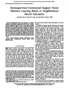
Dependency parsing is one important way to analyse the syntactic structures of natural language. It has been widely studied in the past decade. A dependency parsing task takes natural language (usually tokenised sentence) as input and outputs a sequence of head-dependent relations. Figure 2.1 shows the dependency relations of a sentence (Tom played football with his classmate .) parsed by an off-the-shelf dependency parser. During the past decade, many dependency parsing systems have been introduced, most of them are graph-based or transition-based systems. The graph-based system solves the parsing problem by searching for maximum spanning trees (MST). A first-order MST parser first assigns scores to directed edges between tokens of a sentence. It then uses an algorithm to search a valid dependency tree with the highest score. By contrast, the transition-based system solves the parsing task as a sequence of transition decisions, in

7

P

ADV

ROOT

Tom NNP

NMOD

OBJ

SBJ

PMOD

played VBD

football NN

with IN

his PRP$

classmate NN

Figure 2.1: The dependency relations of the sentence (Tom played football with his classmate .) parsed by Mate parser. each step the parser deciding the next transition. In Section 2.1.1 and 2.1.2 we briefly describe the two major system types. In recent years, deep learning has been playing an important role in the machine learning community. As a result, several neural networkbased systems have been introduced, some of them surpassing the state-of-the-art accuracy achieved by the conventional dependency parsers based on perceptions or SVMs. We briefly touch on neural network-based systems in Section 2.1.3, although most of them are still transition/graph-based systems. The evaluation of the neural network-based parsers is beyond the scope of this thesis, as they become popular after most of the work of this thesis has been done. We mainly use the Mate parser (Bohnet et al., 2013), a transition-based approach that was state-of-the-art at the beginning of this work and whose performance remained competitive even after the introduction of the parsers based on neural network. Section 2.1.4 introduces the technical details of the Mate parser.

2.1.1

Graph-based Systems

The graph-based dependency parser solves the parsing problem by searching for maximum spanning trees (MST). In the following, we consider the first-order MST parser of McDonald et al. (2005). Let x be the input sentence, y be the dependency tree of x, xi is the ith word of x, (i, j) ∈ y is the directed edge between xi (head) and xj (dependent).

8

. .

(1) Build the graph:

Tom

plays

football

40 5

(2) Score the edges:

20

10

Tom

plays 30

football 5

10 40 5

(3) Select highest scoring tree:

20

10

Tom

plays

football

30

5

10 40 20

30

(4) The final parser tree:

Figure 2.2: parser.

Tom

plays

football

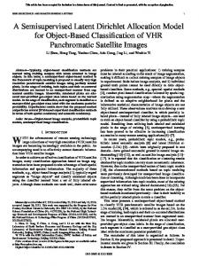
Parsing the sentence (Tom plays football ) with a graph-based dependency

dt(x) is used to represent the set of possible dependency trees of the input sentence where y ∈ dt(x). The parser considers all valid directed edges between tokens in x and builds the parse trees in a bottom-up fashion by applying a CKY parsing algorithm. It scores a parse tree y by summing up the scores s(i, j) of all the edges (i, j) ∈ y. The s(i, j) is calculated according to a high-dimensional binary feature representation f and a weight vector w learned from training data τ (τ = {(xt , yt )}Tt=1 ). To be more specific, the score of a parse tree y of an input sentence x is calculated as follows:

9

s(x, y) =

X

s(i, j) =

(i,j)∈y

X

w ∗ f (i, j)

(i,j)∈y

Where f consists of a set of binary feature representations associated with a number of feature templates. For example, an edge (plays, f ootball) with a bi-gram feature template (headword , depword ) will give a value of 1 for the following feature representation:

f (i, j) =

   1 if headword = “plays” and depword = “f ootball”   0 otherwise

After scoring the possible parse trees dt(x), the parser outputs the highest-scored dependency tree ybest . Figure 2.2 shows an example of a sentence being parsed with a first-order graph-based parser. In terms of training, the parser uses an online learning algorithm to learn the weight vector w from the training set τ . In each training step, only one training instance (xt , yt ) ((xt , yt ) ∈ τ ) is considered, the w is updated after each step. More precisely, the Margin Infused Relaxed Algorithm (MIRA) (Crammer et al., 2006) is used to create a margin between the score of a correct parse tree s(xt , yt ) and the incorrect ones s(xt , y 0 ) (y 0 ∈ dt(xt )). The loss L(yt , y 0 ) of a dependency tree is defined as the number of incorrect edges. Let w(i) , w(i+1) be the weight vector before and after the update of the ith training step, w(i+1) is updated subject to keeping the margin at least as large as the L(yt , y 0 ), while at the same time, keeping the norm of the changes to the w as small as possible. A more detailed training algorithm is showed in algorithm 1. The MST parser is later improved by McDonald and Pereira (2006) to include secondorder features, however, the system is still weaker than its successors which also include third-order features (Koo and Collins, 2010). Other mostly used strong graph-based parsers include Mate graph-based parser (Bohnet, 2010) and Turbo Parser (Martins et al., 2013).

10

1 2 3 4 5 6 7 8 9

Data: τ = {(xt , yt )}Tt=1 Result: w w0 = 0; i = 0; for n : 1..N do // N training iterations for t : 1..T do w(i+1) = update w(i) to min ||w(i+1) − w(i) ||; s.t. s(xt , yt ) − s(xt , y 0 ) ≥ L(yt , y 0 ); ∀y 0 ∈ dt(xt ); i = i + 1; end end Algorithm 1: MIRA algorithm for MST parser

2.1.2

Transition-based Systems

The transition-based parsers build the dependency trees in a very different fashion compared to graph-based systems. Instead of searching for the maximum spanning trees, transition-based systems parse a sentence with a few pre-defined transitions. The Malt parser (Nivre et al., 2007b) is one of the earliest transition-based parsers which has been later widely used by researchers. The parser is well engineered and can be configured to use different transition systems. We take the parser’s default transition system (arc-eager) as an example to show how the transition-based parser works. The Malt parser starts with an initial configuration and performs one transition at a time in a deterministic fashion until it reaches the final configuration. The parser’s configurations are represented by triples c = (Σ, B, A), where Σ is the stack that stores partially visited tokens, B is a list of remaining tokens that are unvisited, and A stores the directed arcs between token pairs that have already been parsed. The parser’s initial configuration consists of an empty Σ and an empty A, while all the input tokens are stored in B. The final configuration is required to have an empty B. A set of four transitions (Shift, Left-Arc, Right-Arc and Reduce) are defined to build the parse trees. The Shift transition moves the token on the top of B into Σ, the Left-Arc transition adds an arc from the top of B to the top of Σ and removes the token on the top of Σ, the Right-Arc transition adds an arc from the top of Σ to the top of B and moves the token on the top of B into Σ, and the Reduce 11

The initial state:

[]

[ Tom

Perform Shift transition:

plays

[ Tom ]

football ]

[ plays

football ]

SBJ

Perform Left-Arc transition:

[

Perform Shift transition:

Tom

[

]

plays

[

]

plays

[

football

football

]

]

OBJ

Perform Right-Arc transition: Perform Reduce transition:

[

[

plays

football ]

(((( ( football

plays

]

[]

[]

ROOT SBJ

The final parse tree:

Tom

plays

OBJ

football

Figure 2.3: Parsing the sentence (Tom plays football ) with an arc-eager transition-based dependency parser. The square brackets denote the stack (left) and the buffer (right) used by transition-based parser. transition simply removes the token on the top of Σ. More precisely, table 2.1 shows the details of the transitions of an arc-eager system. To train the parser, support vector machine classifier (SVM) with the one-versus-all strategy is used to solve the transition-based parser as a multi-classification problem. In a transition-based parsing scenario, the classes are different transitions. Each of the SVMs is trained to maximise the margin between the target transition and the other transitions, as in the one-versus-all strategy the classes other than the target class are treated the same as the negative examples. Since the data may not be linearly separable, they use in additional a quadratic kernel (K(xi , xj ) = (γxTi xj + r)2 ) to map the data

12

Transition Left-Arc Right-Arc Shift Reduce

([σ|i], [j|β], A) ⇒ (σ, [j|β], A ∪ {(j → i)} ([σ|i], [j|β], A) ⇒ ([σ|i|j], β, A ∪ {(i → j)}) (σ, [i|β], A) ⇒ ([σ|i], β, A) ([σ|i], B, A) ⇒ (σ, B, A)

Table 2.1: Transitions for arc-eager parsing. into a higher dimensional space. The SVMs are trained to predict the next transition based on a given parser configuration. They used similar binary feature representations as those of the MST parser, in which the features are mapped into a high dimensional vector. The feature templates for the transition-based system are mainly associated with the configurations, for example, a feature between the Σtop (the top of the stack) and the Btop (the top of the Buffer) is as follows:

fci =

   1 if Σtop = “plays” and Btop = “f ootball”   0 otherwise

Figure 2.3 shows an example of parsing the sentence (Tom plays football ) with the Malt transition-based parser. Benefiting from the deterministic algorithm, the Malt parser is able to parse the nonprojective sentences in linear time (Nivre, 2009), which is much faster compared to the second-order MST parser’s cubic-time parsing (McDonald and Pereira, 2006). Although the deterministic parsing is fast, the error made in the previous transitions will largely affect the decisions taken afterwards, which results in a lower accuracy. To overcome this problem beam search has been introduced to the transition-based systems, which leads to significant accuracy improvements (Bohnet et al., 2013).

2.1.3

Neural Network-based Systems

Neural network-based systems have only been recently introduced to the literature. Chen and Manning (2014) were the first to introduce a simple neural network to a deterministic

13

Figure 2.4: Neural Network architecture taking from Chen and Manning (2014) transition-based parser, yielding good results. The parser used an arc-standard transition system. Similar to arc-eager, the arc-standard is another highly used transition-based system. Many dependency parsers are based on or have options to use an arc-standard approach, which include the Malt parser we introduced in the previous section (section 2.1.2) and our main evaluation parser (Mate parser). We will introduce the arc-standard transition system in more detail in section 2.1.4. One of the major differences between the neural network based systems and the conventional systems is the use of feature representations. Instead of using the binary feature representations (commonly used by the conventional systems), the neural network based approaches represent the features by embeddings. During training, feature embeddings (e.g. word, part-of-speech embeddings) are capable of capturing the semantic information of the features. Take the part-of-speech tags as an example, adjective tags JJ, JJR, JJS will have similar embeddings. This allows the neural network-based systems to reduce the feature sparsity problem of the conventional parser systems. Conventional parsers usually represent different tokens or token combinations by independent feature spaces, thus are highly sparse. Another advantage of using the neural network based approach is that the system 14

allows using the pre-trained word embeddings. Word embeddings extracted from large unlabelled data carry the statistical strength of the words, this could be a better bases for the system when compared to the randomly initialised embeddings. The empirical results confirmed that large improvements can be achieved by using the pre-trained word embeddings. The idea of using the pre-trained word embeddings goes into the same direction of the semi-supervised approaches that use unlabelled data indirectly, such as dependency language models evaluated in this thesis, or word clusters. In terms of the network architecture, Chen and Manning (2014) used a single hidden layer and a softmax layer to predict the next transition based on the current configuration. To map the input layer to the hidden layer they used a cube activation function (h = (W w xw + W t xt + W l xl + b)3 ), in which xw , xt , xl are feature embeddings of the words, part-of-speech tags and arc labels and W w , W t , W l are the relative weights. Figure 2.4 shows the details of their neural network architecture. This first attempt of using the neural network for dependency parsing leads to many subsequent research. Chen and Manning (2014)’s system has been later extended by Weiss et al. (2015) who introduced beam search to the system and achieved state-of-theart accuracy. Since then a number of more complex and powerful neural networks have been evaluated, such as the stack-LSTM (Dyer et al., 2015) and the bi-directional LSTM (Dozat and Manning, 2017). The current state-of-the-art is achieved by the parser of Dozat and Manning (2017) who used the bi-directional LSTM in their system.

2.1.4

The Mate Parser

In this thesis, we mainly used the Mate transition-based parser (Bohnet and Kuhn, 2012; Bohnet and Nivre, 2012; Bohnet et al., 2013). The parser is one of the best performing parsers on the data set of the major shared task (CoNLL 2009) on dependency parsing (Hajiˇc et al., 2009) and it is freely available 1 . The parser uses the arc-standard transition system, it is also integrated with a number of techniques to maximise the parser’s per1

https://code.google.com/p/mate-tools/

15

Transition Left-Arcd Right-Arcd Shiftp Swap

Condition ([σ|i, j], B, A, π, δ) ⇒ ([σ|j], B, A ∪ {(j, i)}, π, δ[(j, i) → d]) i 6= 0 ([σ|i, j], B, A, π, δ) ⇒ ([σ|i], B, A ∪ {(i, j)}, π, δ[(i, j) → d]) (σ, [i|β], A, π, δ) ⇒ ([σ|i], β, A, π[i>], δ) ([σ|i, j], B, A, π, δ) ⇒ ([σ|j], [i|β], A, π, δ) 0 0). Figure 2.5 shows an example of joint tagging and parsing a sentence by the Mate parser. The graph-based completion model consists of a number of different second- and thirdorder feature models to rescore the partial parse tree Treen (x, cn ). Some feature models are similar to Carreras (2007) and Koo and Collins (2010). Take one of the models 2a as an example, which consists of the second-order factors of Carreras (2007): 1. The head and the dependent. 2. The head, the dependent and the right/left-most grandchild in between.

17

Initial state: [ ] [ A hearing is scheduled on the issue ] Shift x 3: [ A/DT hearing/NN ] [ is scheduled on the issue ] DET

hearing/NN ] [ is scheduled on the issue ] Left-Arc: [ A/DT

Shift x 3: [ hearing/NN is/VBZ scheduled/VBN on/IN ] [ the issue ] Swap x 2: [ hearing/NN on/IN ] [ is/VBZ scheduled/VBN the issue ] Shift x 3: [ hearing/NN on/IN is/VBZ scheduled/VBN the/DT ] [ issue ] Swap x 2: [ hearing/NN on/IN the/DT ] [ is/VBZ scheduled/VBN issue ] Shift x 3: [ hearing/NN on/IN the/DT is/VBZ scheduled/VBN issue/NN ] [ ] Swap x 2: [ hearing/NN on/IN the/DT issue/NN] [ is/VBZ scheduled/VBN ] DET

issue/NN] [ is/VBZ scheduled/VBN ] Left-Arc: [ hearing/NN on/IN the/DT NMOD

PC

[ is/VBZ scheduled/VBN ] issue/NN] Right-Arc x 2: [ hearing/NN on/IN

Shift: [ hearing/NN is/VBZ ] [ scheduled/VBN ] SBJ

(

hearing/NN Left-Arc: [ ( (((( is/VBZ ] [ scheduled/VBN ] Shift: [ is/VBZ scheduled/VBN ] [ ] VG ROOT

((

( ( Right-Arc x 2: [ is/VBZ scheduled/VBN ] [] (((( NMOD ROOT PC DET

VG

SBJ

DET

Output: A/DT hearing/NN is/VBZ scheduled/VBN on/NN the/DT issue/NN

Figure 2.5: Parsing the sentence (A hearing is scheduled on the issue) with the Mate transition-based dependency parser. The square brackets denote the stack (left) and the buffer (right) used by transition-based parser. 3. The head, the dependent and the right/left-most grandchild away from the head. 4. The head, the dependent and between those words the right/left-most sibling.

18

1 2 3 4 5 6 7 8 9 10 11 12 13 14 15 16 17 18

Data: (x, w, b) Result: Tree(x, h.c) h0 .c ← cs (x); h0 .s ← 0.0; h0 .f ← {0.0}dim(w) ; Beam ← [h0]; while ∃c ∈ Beam : c ∈ / Ct do Tmp ← [ ]; for h : Beam do for t ∈ T : Permissible(c, t) do h.f ← h.f + f (h.c, t); h.s ← h.s + f (h.c, t) ∗ w; h.c ← t(h.c); Tmp ← Insert(h, Tmp); end end Beam ← Prune(Tmp, b); end h ← Top(Beam); return Tree(x, h.c); Algorithm 2: Beam search algorithm for the Mate parser Feature models are independent to each other and can be easily turned on/off by

configuration. The score of a parse tree Tree(x, c) or a partial parse tree Treen (x, cn ) is then defined as the sum of the scores from the both parts:

Score(x, c) = ScoreT (x, c) + ScoreG (x, c) Where ScoreT (x, c) is the score of the transition-based part of the parser and ScoreG (x, c) is the score from the graph-based completion model. Mate parser uses similar binary feature representations as those of the MST/Malt parser (the features are represented by a high dimensional feature vector (f )). A learned weight vector (w) is used with the feature vector (f ) to score the configurations in conjunction with the next transition. In addition, the parser uses the beam search to mitigate error propagation. Comparing with the deterministic parsing algorithm that only keeps the best partial parse tree, the beam search approach keeps the n-best partial parse trees during the inference. By using the beam search, errors made in the early stage can po19

tentially be recovered in the late stage, as long as the correct configuration has not fallen out of the beam. The beam search algorithm takes a sentence (x), the weight vector (w) and the beam size parameter (b) and returns the best scoring parse tree (Tree(x, h.c)). A parse hypothesis (h) of a sentence consists of a configuration (h.c), a score (h.s) and a feature vector (h.f ). Initially the Beam only consists of the initial hypothesis (h0 ), in which h0 contains a initial configuration of the sentence (cs (x)), a score of 0.0 and a initial feature vector ({0.0}dim(w) ). The transitions (T ) change the hypotheses in steps and create new hypotheses by applying different permissible transitions to them. For each step, the top b scoring hypotheses are kept in the Beam. The beam search terminates when every hypothesis in the Beam contains a terminal configuration (h.c ∈ Ct ). It then returns the top scoring parse tree (Tree(x, h.c)). Algorithm 2 outlines the details of the beam search algorithm used by the Mate parser. In order to learn the weight vector, the parser goes through the training set (τ = {(xt , yt )}Tt=1 ) for N iterations. The weight vector is updated for every sentence xt when an incorrect parse is returned (i.e. the highest scoring parse yt∗ is different from the gold parse yt ). More precisely, the passive-aggressive update of Crammer et al. (2006) is used:

w(i+1) = w(i) +

f (xt , yt ) − f (xt , yt∗ ) ||f (xt , yt ) − f (xt , yt∗ )||2

In this thesis, unless specified, we used the default settings of the parser: 1. We use all the graph-based features of the completion model. 2. We use the joint PoS-tagging with two-best tags for each token. 3. We use a beam of 40. 4. We use 25 iterations of training. 5. We do not change the sentence order of the training data during training.

20

2.2

Out-of-domain Parsing

The release of the large manually annotated Penn Treebank (PTB) (P. Marcus et al., 1993) and the development of the supervised learning techniques enable researchers to work on the supervised learning based parsing systems. Over the last two decades, the parsing accuracy has been significantly improved. A number of strong parsing systems for both constituency and dependency families have been developed (Klein and D. Manning, 2003; Petrov and Klein, 2007; Bohnet et al., 2013; Martins et al., 2013; Weiss et al., 2015; Dozat and Manning, 2017). The parsers based on supervised learning techniques capture statistics from labelled corpora to enable the systems to correctly predict parse trees when input the corresponding sentences. Since the PTB corpus contains mainly texts from news domain, the supervised learning based parsers trained on PTB corpus are sensitive to domain shifting. Those systems are able to achieve high accuracies when tested on the PTB test set (i.e. in-domain parsing). However, when applying them on data from different sources (i.e. out-of-domain parsing), such as web domain (Petrov and McDonald, 2012) and chemical text(Nivre et al., 2007a), the accuracy drops significantly. Table 2.3 shows a comparison of the in-domain and out-of-domain parsing performance of three parsers that have been frequently used by researchers (i.e. MST (McDonald and Pereira, 2006), Malt (Nivre, 2009), and Mate parser (Bohnet et al., 2013)). Those parsers are trained on the training data from the major shared task on dependency parsing (i.e. CoNLL 2009 (Hajiˇc et al., 2009)). The training set contains mainly the news domain data from the Penn Treebank. In our evaluation, we first test them on the CoNLL test set which denotes our in-domain examples; for our out-of-domain examples we test the parsers on a number of different domains from the OntoNotes v5.01 corpus. As we can see from the results, the accuracies on out-of-domain texts are much lower than that of in-domain texts, with the largest accuracy difference of more than 15% (i.e. Mate parser has an accuracy of 90.1% on in-domain texts and an accuracy of 74.4% on texts from broadcast 1

https://catalog.ldc.upenn.edu/LDC2013T19

21

Domain MST Malt Newswire 84.8 81.7 Pivot Texts 84.9 83.0 Broadcast News 79.4 78.1 Magazines 77.1 74.7 Broadcast Conversation 73.4 70.5 CoNLL 86.9 84.7

Mate 87.1 86.6 81.2 79.3 74.4 90.1

Table 2.3: Labelled attachment scores achieved by the MST, Malt, and Mate parsers trained on the Conll training set and tested on different domains. conversations). How can we reduce the accuracy gap between the in-domain and the outof-domain parsing? The most straightforward way would be annotating more text for the target domain, however, this approach is very expensive and time-consuming. There are only very limited manually annotated corpora available, which confirms the high costs of the annotation process. Domain adaptation is a task focused on solving the out-of-domain problems but without the need for manual annotation. There are a number of directions to work on the domain adaptation task, each of them focusing on a different aspect. These directions include semi-supervised techniques, domain specific training data selection, external lexicon resources and parser ensembles. Each direction has its own advantages and disadvantages, we briefly discuss in Section 2.2.1. In this thesis, we mainly focus on one direction that improves the out-of-domain accuracy by using unlabelled data (Semisupervised approaches). Similar to other domain adaptation approaches, semi-supervised approaches do not require to manually annotate new data, but instead, they use the widely available unlabelled data. Some semi-supervised approaches focus on boosting the training data by unlabelled data that is automatically annotated by the base models, others aid the parsers by incorporating features extracted from the large unlabelled data. In Section 2.2.2 we discuss both approaches in detail.

2.2.1

Approaches to Out-of-Domain Parsing

As stated above, the domain adaptation techniques are designed to fill the accuracy gaps between the source domain and the target domain. Previous work on domain adaptation 22

tasks is mainly focused on four directions: semi-supervised techniques (Sarkar, 2001; McClosky et al., 2006b; Reichart and Rappoport, 2007; Sagae and Tsujii, 2007; Koo et al., 2008; Sagae, 2010; Zhou et al., 2011; Zhang et al., 2012), target domain training data selection (Plank and van Noord, 2011; Søgaard and Plank, 2012; Khan et al., 2013), external lexicon resources (Szolovits, 2003; Pyysalo et al., 2006; Pekar et al., 2014) and parser ensembles (Nivre et al., 2007a; Le Roux et al., 2012; Zhang et al., 2012; Petrov and McDonald, 2012). The semi-supervised techniques focus on exploring the largely available unlabelled data. There are two major ways to use the unlabelled data. The first family aims to boost the training data. Data that has been automatically annotated by the base models are used directly in re-training as the additional training set, up-training, self-training and co-training are techniques of this family. The other family uses the features extracted from unlabelled data to aid the base model, this type of techniques include word embeddings, word clusters and dependency language models. In this thesis, we use semi-supervised techniques from both families and we will discuss them in detail in Section 2.2.2. Domain specific training data selection is a technique based on the assumption that similarity methods are able to derive a subset of the source domain training data that fits an individual test domain. Plank and van Noord (2011) investigated several similarity methods to automatically select sentences from training data for the target domain, which gain significant improvements when comparing with random selection. Positive impacts are also found by Khan et al. (2013) when they experimented with training data selection on parsing five sub-genres of web data. The advantage of this technique is that it does not need any extra data, however, it is also restricted to learn only from the source domain training set. Lack of the knowledge of the unknown words is one of the well-known problems faced by domain adaptation tasks, i.e. target domain test sets usually contain more unknown words (vocabularies which did not appear in the training data) than source domain test sets (Nivre et al., 2007a; Petrov and McDonald, 2012) . One way to solve this problem is

23

to use the external lexicon resources created by the linguistics. External lexicons provide additional information for tokens, such as word lemma, part-of-speech tags, morphological information and so on. This information can be used by parsers directly to help making the decision. Previously, lexicons have been used by Szolovits (2003) and Pyysalo et al. (2006) to improve the link grammar parser on the medical domain. Both approaches showed large improvements on parsing accuracy. Recently, Pekar et al. (2014) extracted a lexicon from a crowd-sourced online dictionary (Wiktionary) and applied it to a strong dependency parser. Unfortunately, in their approach, the dictionary achieved a moderate improvement only. The fourth direction of domain adaptation is parser ensembles, it becomes more noticeable, due to its good performance in shared tasks. For example, in the first workshop on syntactic analysis of non-canonical language (SANCL), the ensemble-based systems on average produced much better results than that of single parsers (Le Roux et al., 2012; Zhang et al., 2012; Petrov and McDonald, 2012). However, those ensemble-based systems are not used in real-world tasks, due to the complex architectures and high running time.

2.2.2

Semi-Supervised Approaches

Semi-supervised approaches use unlabelled data to bridge the accuracy gap between indomain and out-of-domain. In recent years, unlabelled data has gained large popularity in syntactic parsing tasks, as it can easily and inexpensively be obtained, cf. (Sarkar, 2001; Steedman et al., 2003; McClosky et al., 2006a; Koo et al., 2008; Søgaard and Rishøj, 2010; Petrov and McDonald, 2012; Chen et al., 2013; Weiss et al., 2015). This is in stark contrast to the high costs of manually labelling new data. Some techniques such as self-training (McClosky et al., 2006a) and co-training (Sarkar, 2001) use autoparsed data as additional training data. This enables the parser to learn from its own or other parsers’ annotations. Other techniques include word clustering (Koo et al., 2008) and word embedding (Bengio et al., 2003) which are generated from a large amount of unlabelled data. The outputs can be used as features or inputs for parsers. Both groups 24

of techniques have been shown effective on syntactic parsing tasks (Zhou and Li, 2005; Reichart and Rappoport, 2007; Sagae, 2010; Søgaard and Rishøj, 2010; Yu et al., 2015; Weiss et al., 2015).

Boosting the Training Set The first group uses unlabelled data (usually parsed data) directly in the training process as additional training data. The most common approaches in this group are co-training and self-training. Co-training is a technique, that has been frequently used by domain adaptation for parsers (Sarkar, 2001; Sagae and Tsujii, 2007; Zhang et al., 2012; Petrov and McDonald, 2012). The early version of co-training uses two different ’views’ of the classifier, each ’view’ has a distinct feature set. Two ’views’ are used to annotate unlabelled set after trained on the same training set. Then both classifiers are retrained on the newly annotated data and the initial training set (Blum and Mitchell, 1998). Blum and Mitchell (1998) first applied a multi-iteration co-training on classifying web pages. Then it was extended by Collins and Singer (1999) to investigate named entity classification. At that stage, co-training strongly depended on the splitting of features (Zhu, 2005). One year after, Goldman and Zhou (2000) introduced a new variant of co-training which used two different learners, but both of them took the whole feature sets. One learner’s high confidence data are used to teach the other learner. After that, Zhou and Li (2005) proposed another variant of co-training (tri-training). Tri-training used three learners, each learner is designed to learn from data on which the other two learners have agreed. In terms of the use of co-training in the syntactic analysis area, Sarkar (2001) first applied the co-training to a phrase structure parser. He used a subset (9695 sentences) of labelled Wall Street Journal data as initial training set and a larger pool of unlabelled data (about 30K sentences). In each iteration of co-training, the most probable n sentences from two views are added to the training set of the next iteration. In their experiments, the parser achieved significant improvements in both precision and recall (7.79% and

25

10.52% respectively) after 12 iterations of co-training. The work most close to ours was presented by (Sagae and Tsujii, 2007) in the shared task of the conference on computational natural language learning (CoNLL). They used two different settings of a shift-reduce parser to complete a one iteration co-training, and their approach successfully achieved improvements of approximately 2-3%. Their outputs have also scored the best in the out-of-domain track (Nivre et al., 2007a). The two settings they used in their experiments are distinguished from each other in three ways. Firstly, they parse the sentences in reverse directions (forward vs backward). Secondly, the search strategies are also not the same (best-first vs deterministic). Finally, they use different learners (maximum entropy classifier vs support vector machine). The maximum entropy classifier learns a conditional model p(y|x) by maximising the conditional entropy P (H(p) = − x,y p˜(x)p(y|x) log p(y|x))1 , while the support vector machines (SVMs) are linear classifiers trained to maximise the margin between different classes. In order to enable the multi-class classification, they used the all-versus-all strategy to train multiple SVMs for predicting the next transition. In addition, a polynomial kernel with degree 2 is used to make the data linearly separable. Sagae and Tsujii (2007) proved their assumptions in their experiments. Firstly, the two settings they used are different enough to produce distinct results. Secondly, the perfect agreement between two learners is an indication of correctness. They reported that the labelled attachment score could be above 90% when the two views agreed. By contrast, the labelled attachment scores of the individual view were only between 78% and 79%. Tri-training is a variant of co-training. A tri-training approach uses three learners, in which the source learner is retrained on the data produced by the other two learners. This allows the source learner to explore additional annotations that are not predicted by its own, thus it has a potential to be more effective than the co-training. Tri-training is used by (Zhang et al., 2012) in the first workshop on syntactic analysis of non-canonical language (SANCL)(Petrov and McDonald, 2012). They add the sentences which the two 1

p˜(x) is the empirical distribution of x in the training data.

26

parsers agreed on into the third parser’s training set, then retrain the third parser on the new training set. However, in their experiments, tri-training did not significantly affect their results. Recently, Weiss et al. (2015) used normal agreement based co-training and tri-training in their evaluation of a state-of-the-art neural network parser. Their evaluation is similar to the Chapter 3 of this thesis, although they used different parsers. Please note their paper is published after our evaluation on co-training (Pekar et al., 2014). In their work, the annotations agreed by a conventional transition-based parser (zPar) (Zhang and Nivre, 2011) and the Berkeley constituency parser (Petrov and Klein, 2007) have been used as additional training data. They retrained their neural network parser and the zPar parser on the extended training data. The neural network parser gained around 0.3% from the tri-training, and it outperforms the state-of-the-art accuracy by a large 1%. By contrast, their co-training evaluation on the zPar parser found only negative effects. Self-training is another semi-supervised technique that only involves one learner. In a typical self-training iteration, a learner is firstly trained on the labelled data, and then the trained learner is used to label some unlabelled data. After that, the unlabelled data with the predictions (usually the high confident predictions of the model) are added to the training data to re-train the learner. The self-training iteration can also be repeated to do a multi-iteration self-training. When compared with co-training, self-training has a number of advantages. Firstly unlike the co-training that requires two to three learners, the self-training only requires one learner, thus it is more likely we can use the self-training than co-training in an under resourced scenario. Secondly, to generate the additional training data, co-training requires the unlabelled data to be double annotated by different learners, this is more time-consuming than self-training’s single annotation requirement. In term of the previous work on parsing via self-training, Charniak (1997) first applied self-training to a PCFG parser, but this first attempt of using self-training for parsing failed. Steedman et al. (2003) implemented self-training and evaluated it using several settings. They used a 500 sentences training data and parsed only 30 sentences in each

27

self-training iteration. After multiple self-training iterations, it only achieved moderate improvements. This is caused probably by the small number of additional sentences used for self-training. McClosky et al. (2006a) reported strong self-training results with an improvement of 1.1% f-score by using the Charniak-parser, cf. (Charniak and Johnson, 2005). The Charniak-parser is a two stage parser that contains a lexicalized context-free parser and a discriminative reranker. They evaluated on two different settings. In the first setting, they add the data annotated by both stages and retrain the first stage parser on the new training set, this results in a large improvement of 1.1%. In the second setting, they retrain the first stage parser on its own annotations, the result shows no improvement. Their first setting is similar to the co-training as the first stage parser is retrained on the annotation co-selected by the second stage reranker, in which the additional training data is more accurate than the predictions of first stage parser. McClosky et al. (2006b) applied the same method later on out-of-domain texts which show good accuracy gains too. Reichart and Rappoport (2007) showed that self-training can improve the performance of a constituency parser without a reranker for the in-domain parsing. However, their approach used only a rather small training set when compared to that of McClosky et al. (2006a). Sagae (2010) investigated the contribution of the reranker for a constituency parser in a domain adaptation setting. Their results suggest that constituency parsers without a reranker can achieve statistically significant improvements in the out-of-domain parsing, but the improvement is still larger when the reranker is used. In the workshop on syntactic analysis of non-canonical language (SANCL) 2012 shared task, self-training was used by most of the constituency-based systems, cf. (Petrov and McDonald, 2012). The top ranked system is also enhanced by self-training, this indicates that self-training is probably an established technique to improve the accuracy of constituency parsing on out-of-domain data, cf. (Le Roux et al., 2012). However, none of

28

the dependency-based systems used self-training in the SANCL 2012 shared task. One of the few successful approaches to self-training for dependency parsing was introduced by Chen et al. (2008). They improved the unlabelled attachment score by about one percentage point for Chinese.Chen et al. (2008) added parsed sentences that have a high ratio of dependency edges that span only a short distance, i.e. the head and dependent are close together. The rationale for this procedure is the observation that short dependency edges show a higher accuracy than longer edges. Kawahara and Uchimoto (2008) used a separately trained binary classifier to select reliable sentences as additional training data. Their approach improved the unlabelled accuracy of texts from a chemical domain by about 0.5%. Goutam and Ambati (2011) applied a multi-iteration self-training approach on Hindi to improve parsing accuracy within the training domain. In each iteration, they add a small number (1,000) of additional sentences to a small initial training set of 2,972 sentences, the additional sentences were selected due to their parse scores. They improved upon the baseline by up to 0.7% and 0.4% for labelled and unlabelled attachment scores after 23 self-training iterations. While many other evaluations on self-training for dependency parsing are found unhelpful or even have negative effects on results. Plank (2011) applied self-training with single and multiple iterations for parsing of Dutch using the Alpino parser (Malouf and Noord, 2004), which was modified to produce dependency trees. She found self-training produces only a slight improvement in some cases but worsened when more unlabelled data is added. Plank and Søgaard (2013) used self-training in conjunction with dependency triplets statistics and the similarity-based sentence selection for Italian out-of-domain parsing. They found the effects of self-training are unstable and does not lead to an improvement. Cerisara (2014) and Björkelund et al. (2014) applied self-training to dependency parsing on nine languages. Cerisara (2014) could only report negative results in their selftraining evaluations for dependency parsing. Similarly, Björkelund et al. (2014) could

29

observe only on Swedish a positive effect.

Integrating with Features Learned from Unlabelled Data The second group uses the unlabelled data indirectly. Instead of using the unlabelled data as training data, they incorporate the information extracted from large unlabelled data as features to the parser. Word clusters (Koo et al., 2008; Cerisara, 2014) and word embeddings (Chen and Manning, 2014; Weiss et al., 2015) are most well-known approaches of this family. However, other attempts have also been evaluated, such as dependency language models (DLM) (Chen et al., 2012). Word Clustering is an unsupervised algorithm that is able to group the similar words into the same classes by analysing the co-occurrence of the words in a large unlabelled corpus. The popular clustering algorithm includes Brown (Brown et al., 1992; Liang, 2005) and the Latent dirichlet allocation (LDA) (Chrupala, 2011) clusters. Koo et al. (2008) first employed a set of features based on brown clusters to a secondorder graph-based dependency parser. They evaluated on two languages (English and Czech) and yield about one percentage improvements for both languages. The similar features have been adapted to a transition-based parser of Bohnet and Nivre (2012). The LDA clusters have been used by Cerisara (2014) in the workshop on statistical parsing of morphologically rich languages (SPMRL) 2014 shared tasks (Seddah et al., 2014) on parsing nine different languages, their system achieved the best average results across all non-ensemble parsers. Word embeddings is another approach that relies on the co-occurrence of the words. Instead of assigning the words into clusters, word embedding represent words as a low dimensional vector (such as 50 or 300 dimensional vector), popular word embedding algorithms include word2vec (Mikolov et al., 2013) and global vectors for word representation (GloVe) (Pennington et al., 2014). Due to the nature of the neural networks, word embeddings can be effectively used in the parsers based on neural networks. By using pre-trained word embeddings the neural network-based parsers can usually achieve a higher accuracy

30

compared with those who used randomly initialised embeddings (Chen and Manning, 2014; Weiss et al., 2015; Dozat and Manning, 2017). Other Approaches that use different ways to extract features from unlabelled data have also been reported. Mirroshandel et al. (2012) used lexical affinities to rescore the n-best parses. They extract the lexical affinities from parsed French corpora by calculating the relative frequencies of head-dependent pairs for nine manually selected patterns. Their approach gained a labelled improvement of 0.8% over the baseline. Chen et al. (2012) applied high-order DLMs to a second-order graph-based parser. This approach is most close to the Chapter 6 of this thesis. The DLMs allow the new parser to explore higher-order features without increasing the time complexity. The DLMs are extracted from a 43 million words English corpus (Charniak, 2000) and a 311 million words corpus of Chinese (Huang et al., 2009) parsed by the baseline parser. Features based on the DLMs are used in the parser. They gained 0.66% UAS for English and an impressive 2.93% for Chinese. Chen et al. (2013) combined the basic first- and second-order features with meta features based on frequencies. The meta features are extracted from auto-parsed annotations by counting the frequencies of basic feature representations in a large corpus. With the help of meta features, the parser achieved the state-of-the-art accuracy on Chinese.

2.3

Corpora

As mentioned previously, one contribution of this thesis is evaluating major semi-supervised techniques in a unified framework. For our main evaluation, we used English data from the conference on computational natural language learning (Conll) 2009 shared task (Hajiˇc et al., 2009) as our source of in-domain evaluation. For out-of-domain evaluation, we used weblogs portion of OntoNotes v5.01 corpus (Weblogs) and the first workshop on syntactic analysis of non-canonical language shared task data (Newsgroups,Reviews,Answers) 1

https://catalog.ldc.upenn.edu/LDC2013T19

31

train Conll 39,279 958,167 24.39

Sentences Tokens Avg. Length

test Conll 2,399 57,676 24.04

Table 2.4: The size of the source domain (Conll) training and test sets for our main evaluation corpora.

Source Sentences Tokens Avg. Length

dev test Weblogs Weblogs Newsgroups Reviews OntoNotes OntoNotes SANCL SANCL 2,150 2,141 1,195 1,906 42,144 40,733 20,651 28,086 19.6 19.03 17.28 14.74

Answers SANCL 1,744 28,823 16.53

Table 2.5: The size of the target domain test datasets for our main evaluation corpora. (Petrov and McDonald, 2012). Section 2.3.1 introduces our main evaluation corpora in detail. For comparison and multi-lingual evaluation, we also evaluated some of our approaches in various additional corpora. Our self-training approach has been evaluated on chemical domain data (Chemical) from the conference on computational natural language learning 2007 shared task (Nivre et al., 2007a) and nine languages datasets from the workshop on statistical parsing of morphologically rich languages (Spmrl) 2014 shared task(Seddah et al., 2014). Our dependency language models approach has been evaluated in addition on Wall Street Journal portion of Penn English Treebank 3 (Wsj) (P. Marcus et al., 1993) and Chinese Treebank 5 (Ctb) (Xue et al., 2005). As both treebanks do not contain unlabelled data, we used the data of Chelba et al. (2013) and the Xinhua portion of Chinese Gigaword Version 5.0

1

for our English and Chinese tests respectively.

We introduce those corpora in the experiment set-up section of the relevant chapters.

32


Weblogs 513,687 9,882,352 19.24

unlabelled Newsgroups Reviews Answers 512,000 512,000 27,274 9,373,212 7,622,891 424,299 18.31 14.89 15.55

Table 2.6: The size of unlabelled datasets for our main evaluation corpora.

2.3.1

The Main Evaluation Corpora

In this section, we introduce our main evaluation corpora that have been used in all of the semi-supervised approaches evaluated in this thesis. The Conll English corpus built on the Penn English Treebank 3 (P. Marcus et al., 1993) which contains mainly Wall Street Journals but also included a small portion of Brown corpus(Francis and Kucera, 1979). The training set contains only Wall Street Journals, the small subset of the Brown corpus has been included in the test set. The constituency trees from Penn English Treebank are converted to dependency representation by the LTH constituent-to-dependency conversion tool, cf. (Johansson and Nugues, 2007). A basic statistic of the corpus can be found in Table 2.4. For our Weblogs domain test we used the Ontonotes v5.01 corpus. The Ontonotes corpus contains various domains of text such as weblogs, broadcasts, talk shows and pivot texts. We used the last 20% of the weblogs portion of the Ontonotes v5.0 corpus as our target domain development set and the main test set. The selected subset allows us to build sufficient sized datasets similar to the source domain test set. More precisely, the first half of the selected corpus is used as a test set while the second half is used as the development set. Table 2.5 shows some basic statistic of those datasets. Newsgroups, Reviews and Answers domain data are used as additional test sets for our evaluation. Those additional test domains are provided by the first workshop on syntactic analysis of non-canonical language (SANCL) shared task (Petrov and McDonald, 2012). The shared task is focused on the parsing English web text, in total, they prepared 1 1

https://catalog.ldc.upenn.edu/LDC2011T13 https://catalog.ldc.upenn.edu/LDC2013T19

33

five web domain datasets, two of them are development datasets (Email, Weblogs) and the other three (Newsgroups, Reviews and Answers) are used as test sets. For each of the domains, a small labelled set and a large unlabelled set are provided. In this thesis, we used all three test datasets (both labelled and unlabelled data). In addition, one of the unlabelled texts (Weblogs) from the development portion of the shared task is also used. We used for each domain a similar sized unlabelled dataset to make the evaluation more unified. The only exception is the answers domain, as its unlabelled dataset is much smaller than the other three domains, thus we used all of the data provided. A basic statistic of the labelled test sets and unlabelled data can be found in Table 2.5 and 2.6 respectively. In term of the dependency representation, we used the LTH conversion for our main evaluation corpora. Same as the CoNLL 2009 shared task we converted all the labelled data from constituent trees to dependency representation by the LTH constituent-todependency conversion tool (Johansson and Nugues, 2007) when needed.

2.4

Evaluation Methods

To measure the parser’s performance, we report labelled attachment scores (LAS) and unlabelled attachment scores (UAS). For our evaluation on the main corpora, we use the official evaluation script of the CoNLL 2009 shared task, in which all punctuation marks are included in the evaluation. The LAS and UAS are the standard ways to evaluate the accuracy of a dependency parser. Due to the single-head property of the dependency trees, the dependency parsing can be seen as a tagging task, thus the single accuracy metric is well suited for the evaluation. Both LAS and UAS measure the accuracy by calculating the percentage of the dependency edges that have been correctly attached. The UAS considers an edge is correct if the attachment is correct, it does not take the label into account, while the LAS counts only the edges that are both correctly attached and the correct label also assigned. The LAS is more strict than UAS thus we mainly focus on

34

LAS in our evaluation. Let Ca be the number of edges that are correctly attached, Ca+l be the number of edges that are both correctly attached and have the correct label, Ct be the total number of edges, we compute:

U nlabelled attachment score (U AS) = Ca / Ct

(2.1)

Labelled attachment score (LAS) = Ca+l / Ct

(2.2)

For significance testing, we use the randomised parsing evaluation comparator from a major shared task on dependency parsing (Nivre et al., 2007a) . The script takes predictions annotated by two different models of the same dataset. Let the first input be the one which has a higher overall accuracy. The null hypothesis of the script is that the accuracy difference between the first input and the second input is not statistically significant. And the p-values represent the probability that the null hypothesis is correct. We use the script’s default setting of 10,000 iterations (itotal ), for each iteration, the comparator randomly selects one sentence from the dataset and compares the accuracies of the sentence predicted in the two different inputs. Let iless be the number of randomly selected instances that are predicted less accurately in the first input when compared to the predictions in the second input. The p-value is calculated by:

p=

iless itotal

We mark the significance levels based on their p-values, * for p < 0.05, ** for p < 0.01.

2.5

Analysis Techniques

To understand the behaviour of our methods, we assess our results on a number of tests. We analyse the results on both token level and sentences level. For token level, we focus on the accuracies of individual syntactic labels and the known/unknown words accuracies. For sentence level, we used the methods from McClosky et al. (2006a) to evaluate sentences 35

Accuracy Change (%)

1.5

1

0.5

0

Recall

C O L

O N J C

E P D

P

D R O

T M

V C

Precision

C O

E N A M

A D V

O T

J B O

R O

J SB

O

D

P P M

N

M

O

D

−0.5

F-score

Figure 2.6: The bar chart used to visualise our analysis on individual labels. in four factors. We used all four factors from their analysis, i.e. sentence length, the number of unknown words, the number of prepositions and number of conjunctions. Token Level Analysis. Our token level analysis consists of two tests, the first test assesses the accuracy changes for individual labels. The goal of this test is to find out the effects of our semi-supervised methods on different labels. For an individual label, we calculate the recall, precision and the f-score. Let PL be the number of the label L predicted by the parser, GL be the count of label L presented in the gold data and P GL be the number of the label predicted correctly. The precision (P reL ), recall (RecL ) and the f-score (FL ) are calculated as follows:

P reL = P GL / PL

(2.3)

RecL = P GL / GL

(2.4)

FL = 2 ∗

P reL ∗ RecL P reL + RecL

(2.5)

We compute for each label, the score differences between our enhanced model and 36

100 Better Better Worse Worse No. of Sents

60

2,000

40 1,000 20 0

0

1 2 3 Number of Unknown Words

4

Number of Sentences

80 Percentage (%)

3,000

No Change Change No

0

Figure 2.7: An example of our sentence level analysis on different number of unknown words per sentence. the base model. The results for the most frequent labels are visualised by the bar chart. Figure 2.6 is an example of the bar chart we used, the x-axis shows the names of the relevant label, the y-axis shows the accuracy changes in percentage. For each of the labels, we report the accuracy changes of all three scores (recall, precision and f-score), the left (blue) bar represents the recall, the middle (red) bar represents the precision and the right (brown) bar is for f-score. The second test assesses the overall accuracy of known words and unknown words. The unknown words are defined as the words that are not presented in the initial training set. The initial training set is the one we used to train the base model. To compute the accuracy for known and unknown words, we first assign all the tokens in the dataset into two groups (known and unknown) and then we calculate the labelled and unlabelled accuracies for each of the groups separately. We compare the improvements achieved by our enhanced model on known and unknown words to understand the ability of our model on handling unknown words. Sentence Level Analysis. For our sentence level analysis, we evaluate on four factors (sentence length, the number of unknown words, the number of prepositions and

37

the number of conjunctions) that are known to be problematic in parsing. We use a method similar to McClosky et al. (2006a) in our analysis. For each of the factors, we assign sentences to different classes according to their property, sentences that have the same property are assigned to the same class. Take unknown words factor as an example, sentences which contain the same number of unknown words are grouped together. For each group, we calculate the percentage of sentences that are improved, worsened or unchanged in accuracy by our enhanced model. The reason for using the percentage instead of the number of sentences that were used by McClosky et al. (2006a) is mainly because the absolute numbers vary greatly both within the factor and between factors, thus is not suitable for comparison. The percentage, on the other hand, can be easily compared. In addition to the above values, we also report the number of the sentences in each class. Figure 2.7 shows an example of our sentence level analysis on the different number of unknown words per sentence. The x-axis shows the conditions of the classes. In this example, it represents the different number of unknown words in a single sentence. The y-axis to the left is the percentage and the y-axis to the right is the number of sentences. The blue dashed line represents the percentage of the sentences that are parsed better by our enhanced model, the red dotted line represent the portion that is parsed less accurate, the black dash-dotted line shows the portion of sentences whose accuracy are unchanged. The black solid line is the number of sentences in the individual classes.

2.6

Chapter Summary

This chapter introduced the background and the experiment set-up. The first part focused on dependency parsers, it introduced three major types of dependency parsers and gave a detailed introduction of the base parser used in this thesis. The second part discussed the problem caused by parsing out-of-domain text and the techniques that have been used by previous work to solve the problem. The third part introduced the corpora we used. The last two parts showed our evaluation methods and analysis techniques.

38

CHAPTER 3

CO-TRAINING

In this chapter, we introduce our co-training approach. Co-training is one of the popular semi-supervised techniques that has been applied to many natural language processing tasks, such as named entity recognition (Collins and Singer, 1999), constituency parsing (Sarkar, 2001) and dependency parsing (Sagae and Tsujii, 2007; Petrov and McDonald, 2012). Although co-training approaches are popular, they do not always bring positive effects (Zhang et al., 2012; Weiss et al., 2015). Improvements on results are usually reported by learners that are carefully designed to be as different as possible. Such as in Sagae and Tsujii (2007)’s approach, they form the co-training with parsers consisting of different learning algorithms and search strategies. However, off-the-shelf parsers use many similar features, the output of these parsers are more likely to agree with each other. Thus it is unclear whether the off-the-shelf parsers are suitable for co-training. In this work we evaluate co-training with a number of off-the-shelf parsers that are freely available to the research community, namely Malt parser (Nivre, 2009), MST parser (McDonald and Pereira, 2006), Mate parser (Bohnet et al., 2013), and Turbo parser (Martins et al., 2010). We evaluate those parsers on agreement based co-training algorithms. The evaluation learner is retrained on the training set that is boosted by automatically annotated sentences agreed by two source learners. We investigate both normal agreement based co-training and a variant called tri-training. In a normal co-training setting the evaluation learner is used as one of the source learners, and in a tri-training scenario, the source learners are different from the evaluation learner. 39

In the following sections we introduce our approaches in Section 3.1. We then introduce our experiment settings and results in Section 3.2 and Section 3.3 respectively. After that, in Section 3.4 we analyse the results and trying to understand how co-training helps. In the last section (Section 3.5), we summarise our finding.

3.1

Agreement Based Co-training

In this work, we apply an agreement based co-training to out-of-domain dependency parsing. Our agreement based co-training is inspired by the observation from Sagae and Tsujii (2007) in which the two parsers agreeing on an annotation is an indication of a higher accuracy. We proposed two types of agreement based approaches: one uses parser pairs (normal co-training), the other uses three parsers which is also known as tri-training. Two approaches use a similar algorithm, which involves two source learners and one evaluation learner. Two source learners are used to produce additional training data for retraining the evaluation learner. More precisely, our algorithm is as follows: 1. Two source learners are trained separately on the source domain training set to generate two base models. 2. Both models are used to parse a large number of target domain unlabelled data. 3. After that, we compare two automatically labelled predictions for each of the sentences, the first N (such as 10k, 20k) predictions that both models agreed are added to the end of the source domain training set. 4. Finally, we retrain the evaluation learner on the boosted training set generated in step 3. Although both approaches share the similar algorithm, the major differences between them are: both parsers involved by normal co-training are used as the source learners, in which one of them is also used as the evaluation learner; by contrast, tri-training uses 40

Malt MST Turbo Mate LAS (Single) 72.63 75.35 74.85 77.54 LAS (Identical) 89.32 89.08 90.48 Identical rate 19.81 20.32 22.28 Avg. Length 8.92 9.03 8.96 Table 3.1: The analysis of identical annotations on Weblogs development set. three parsers in total, in which two of them are used as the source learners and the third one is used as the evaluation learner. In terms of parsers selection, we selected four public available dependency parsers, which include two benchmark parsers (Malt parser (Nivre, 2009) and MST parser (McDonald and Pereira, 2006)), one transition-based Mate parser (Bohnet et al., 2013), and one graph-based Turbo parser (Martins et al., 2010). These parsers have been widely used by researchers. A more detailed discussion of the dependency parser can be found in section 2.1. The agreement based co-training depends on the assumption that identical annotations between two learners indicate the correctness. To confirm the suitability of selected parsers, in the preliminary evaluation we assessed the accuracy of identical analysis generated by parser pairs. Because we intend to use the Mate parser as our evaluation parser, we paired each of the other three parsers with Mate parser to create three co-training pairs. We assess our assumption by annotating our Weblogs development set, the development set is parsed by all four parsers. We then extract the identical annotations (whole sentence) from parser pairs. We show the accuracy of individual parsers and the accuracy of identical annotations in Table 3.1. The second row shows the labelled accuracy of each parser on the Weblogs development set. The third row shows the labelled accuracy of the identical annotations between the named parser and Mate parser. The fourth row shows the agreement rate of the parser pairs. The last row shows the average sentence length of the identical annotations. As we can see from the table, our assumption is correct on all the parser pairs. Actually, when they agreed on the annotations, the accuracies can be 16% higher than that of individual parsers. However, we also noticed 41

that the average sentence length of the identical annotations is in stark contrast with that of the entire development set (19.6 tokens/sentence). We will discuss this potential conflict in the later section.

3.2

Experiment Set-up

In our evaluation on co-training we use our main evaluation corpora that consists of a source domain training set (Conll), a Weblogs domain development set, a in-domain test set (Conll) and four out-of-domain test sets (Weblogs, Newsgroups, Reviews and Answers). For each target domains, we used in addition a large unlabelled dataset to supply the additional training set. We evaluate various different settings on the development set to tune the best configuration, after that, we apply the best setting to all the test domains. As mentioned before, we used four parsers in our experiments. cf. the Malt parser (Nivre, 2009), MST parser (McDonald and Pereira, 2006), Mate parser (Bohnet et al., 2013), and the Turbo parser (Martins et al., 2010). We use the default settings for all the parsers. The part-of-speech tags is annotated by Mate parser’s internal tagger. To create the additional training corpus, the unlabelled datasets are annotated by all the parsers which are trained on the Conll source domain training set. The Mate parser is used as our evaluation learner, the baseline for all the domains are generated by Mate parser trained on the same Conll training set and applied directly to target domains. We mainly report the labelled attachment scores (LAS), but also include the unlabelled attachment scores (UAS) for our evaluations on test sets. We mark the significance levels according to the p-values, * indicates significance at the p < 0.05 level, ** for the p < 0.01 level.

42

3.3

Empirical Results

Agreement based co-training. We first evaluate the parser pairs on the normal agreement based co-training. Each of the other three parsers is paired with Mate parser to be the source learners of our co-training. For each pairwise parser combinations, the unlabelled Weblogs text is double parsed by the parser pairs. The sentences that are annotated identically by both parsers are used as candidates for the additional training set. We take different amount of additional training sentences from the candidates pool to retrain the Mate parser. Figure 3.1 shows the co-training results of adding 10k to 30k additional training data for all three parser pairs. As we can see from the figure, all the co-training results achieved improvements when compared with the Mate baseline. The largest improvement of one percentage point is achieved by Mate-Malt parser pair when adding 20k or 30k additional training data. We also notice a negative correlation between the improvement and the identical rate mentioned previously in Table 3.1. The Turbo parser has the highest identical rate, in which it annotated 479 out of 2150 sentences (22.28%) exactly the same as Mate parser when evaluated on the development set. This is 2% higher than that of MST parser and 2.5% higher than the Malt parser. However, the improvements achieved by the pairs are shown to be negatively correlated, i.e. the Mate-Malt pair gains the largest improvement, the Mate-Turbo pair achieved the lowest gain. This finding is in-line with the fundamental of co-training that requires the learners to be as different as possible. Removing short sentences from identical data. The identical annotations between the parsers are like a double-edged sword, they consist of a higher accuracy but in the same time shorter in average sentence length. Take our Mate-Malt pair as an example, the average sentence length of the identical annotations is only 8 tokens, this is much lower than the development set’s 19.6 tokens/sentence and the Conll training set’s 24.4 tokens/sentence. To make the additional training data more similar to the manually annotated data, we exclude the extremely short sentences from the pool. More precisely

43

Labeled Attachment Score (%)

80 Mate-Malt Mate-MST Mate-Turbo Mate Baseline

79

78

77

10

20 30 Additional Training Data (K)

Figure 3.1: The results of our normal agreement-based co-training with three different parser pairs. >6 tokens >5 tokens >4 tokens All sentences

LAS (Identical) Avg. Length Identical Sentences 89.44 13.1 248 89.29 12.67 278 89.19 11.94 311 89.32 8.35 426

Table 3.2: The quantity and quality (LAS) of identical (Mate-Malt) development set sentences when omitting the short sentences. we set three minimal sentence length thresholds (4, 5 and 6 tokens), sentences shorter than the thresholds are removed from the pool. We then take 30k sentences from the remaining pool as the additional training data. By taking out the short sentences the average sentence length of the selected sentences is closer to that of the development set. As shown in Table 3.2, the average sentence length reached 13 tokens/sentence. One of the major concerns when we exclude the short sentences from the pool is that the accuracy of the remaining pool might drop. The short sentences are easier to parse, thus they usually have a higher accuracy. However, an evaluation on the development set shows that there is almost no effect on the accuracies (see Table 3.2). In term of the results, we gained a 0.27% additional improvement when discarding short sentences (Figure 3.2).

44


80 Exclude Short Sentences All Sentences

79.5

79

78.5

78

4

5 Mininum Sentence Length

6

Figure 3.2: The effect of omitting short sentences from additional training data. Three learners co-training. In the normal co-training setting, the Mate parser is used as one of the source learners to provide additional training data for retraining itself. Based on this setting the Mate parser can learn only from the annotations it has already known. The tri-training algorithm is on the other hand designed to allow the evaluation learner to learn from sources other than itself. This gives the Mate parser the potential to explore novel examples from other parsers. In our tri-training experiments, we used the Malt parser and the MST parser as our source learners. The sentences that are annotated identically by these parsers are added to the pool for retraining the Mate parser. To assess the quality of the identical annotations between Malt and MST parsers we apply them to our development set. We also assessed the sentences that are annotated identically by Malt and MST parsers but different to Mate parser’s annotation, this allows us to know the scale of the novel examples. As shown in Table 3.3, the accuracy of the sentences agreed by Malt and MST parsers is even slightly higher than that of Mate and Malt parsers, this is surprising as MST parser is less accurate than Mate parser. The analysis also showed that half of the identical annotations from Malt and MST parsers are actually novel to Mate parser. We compared our tri-training and co-training results in Figure 3.3, the tri-training results constantly outperform the normal co-training. The best result of 45

Mate-Malt Malt-MST Malt-MST excl. Mate

LAS (Identical) Identical Sentences 89.44 248 90.20 300 89.28 147

Table 3.3: The quantity and quality (LAS) of identical development set sentences agreed by different parser pairs. Labeled Attachment Score (%)

80 Tri-training Normal Co-training Mate Baseline

79

78

77

10

20 30 40 Additional Training Data (K)

Figure 3.3: The results of our tri-training compared with normal co-training. 79.12% is achieved by retraining the Mate parser with 20k additional training data agreed by Malt-MST parsers (tri-training). The best tri-training result is 0.24% higher than that of co-training and nearly 1.6% higher than the Mate baseline. Evaluating on test domains.

We then evaluated our best configuration (tri-

training) on our four test domains. Under the tri-training setting, the unlabelled datasets of each domain are double parsed by Malt-MST pairs, the first 20k identical annotations are used as additional training data to retrain the Mate parser. The only exception is for answers domain. Due to the lack of unlabelled data the additional training data is much smaller, we used all 3k identical sentences for retraining. Table 3.4 shows our tri-training results accompanied by the baselines. The tri-training setting achieved large labelled improvements up to 1.8 percentage points. For unlabelled attachment scores, the models gained up to 0.59% absolute improvements. We also tested the retrained Weblogs do46

Tri-training LAS UAS Weblogs 80.59** 85.61** Newsgroups 76.44** 83.13 Reviews 76.87** 83.27** Answers 74.59** 81.58 Conll 90.16 92.47

Baseline LAS UAS 78.99 85.1 75.3 82.88 75.07 82.68 73.08 81.15 90.07 92.4

Table 3.4: The effect of applying the best configuration (tri-training) to our test domains. main model on the in-domain test set. The results show the tri-trained model does not affect the in-domain accuracy.

3.4

Analysis

From the above experiments, we demonstrated the effect of co-/tri-training on parsing out-of-domain text with the off-the-shelf parsers. It remains unclear how the additional training data helps the target domain parsing. To understand where the improvements come from, in this section we give a detailed study on the results. We compare the annotations produced by our tri-training approach and the baseline and evaluate the changes on both token level and sentence level. For our analysis, we treat all the target domain as the same, the Weblogs, Newsgroups, Reviews and Answers domain test sets are used as a single set.

3.4.1

Token Level Analysis

Individual Label Accuracy. We first compared the individual label accuracies of the tri-trained model and the baseline. For each of the label we calculate recalls, precisions and f-scores, we then compute the score differences between the tri-trained model and the baseline model. Table 3.4 shows the score changes of the most frequent labels. All the f-scores of our tri-trained model outperform the baseline, the only exception is the P (punctuations) which drops slightly by 0.1%. Eight labels achieved around 0.5% improvements which include ROOT (root of the sentence), SBJ (subject), COORD (coordination), 47

Confusion NMOD → ADV NMOD → LOC NMOD → HYPH NMOD → NAME NMOD → PMOD NMOD → HMOD NMOD → ROOT,OBJ,SBJ,DEP P → HYPH P → NAME,NMOD SBJ → NMOD SBJ → OBJ OBJ → NMOD OBJ → SBJ PMOD → NMOD PMOD → OBJ ROOT → NMOD ROOT → OBJ,SBJ ADV → MNR ADV → AMOD ADV → LOC ADV → NMOD ADV → TMP ADV → DIR COORD → NMOD COORD → ROOT VC → OPRD CONJ → NMOD DEP → ROOT DEP → OBJ DEP → SBJ DEP → NMOD DEP → TMP DEP → ADV AMOD → ADV AMOD → NMOD AMOD → HYPH TMP → ADV TMP → NMOD PRD → OBJ PRD → ADV,VC

Baseline tri-training 235 229 162 164 198 196 569 583 187 179 217 213 491 442 162 173 233 245 169 157 132 72 218 202 117 89 290 275 122 92 235 235 256 216 150 129 152 134 227 214 382 373 182 195 118 113 164 140 102 94 114 23 132 130 190 199 267 241 403 420 382 396 176 165 142 133 169 157 265 273 104 105 280 268 133 128 854 97 255 184

Table 3.5: The confusion matrix of dependency labels, compared between the tri-training approach and the baseline.

48

Precision

Accuracy Change (%)

D P R

B J O

P T M

A M

D

C

O N J

R C O O

R O O

M O P

O M N

Recall

O D

0

E P

0

V C

10

D

1

A D V

20

T

2

D

30

SB J

3

P

40

D

Accuracy Change (%)

4

F-score

Figure 3.4: The performance comparison between the tri-training approach and the baseline on major labels. The x-axis shows the labels, the y-axis to the left shows the accuracy changes for labels from start to TMP, the y-axis to the right-hand side is for label OBJ and PRD only. CONJ (conjunct), modifiers (NMOD (modifier of nominal), PMOD (modifier of preposition), AMOD (modifier of adjective or adverbial)) and DEP (unclassified relations). ADV (adverbial), VC (verb chain) and TMP (temporal adverbial or nominal modifier) are labels that have improvements between 1% and 2%. The accuracy changes are much larger for label OBJ and PRD, thus we used a secondary y-axis for them. More precisely, an improvement of 5.9% is found on OBJ (object), a much better precision of 10% suggests this improvement is mainly contributed by the reduced false positive. The largest improvement of 15% comes from label PRD (predicative complement), the improvement is as a result of significant recall change. The baseline parser can only recall 43% of the label, it has been improved significantly (34%) by the tri-trained model. Table 3.5 shows the confusion matrix of dependency labels. As we can see from the table, the PRD has been frequently labeled as OBJ by the baseline, but this has been largely corrected by our tri-training model.

49

Tri-training Baseline Tokens LAS UAS LAS UAS Known 101616 78.7 84.5 77.1 84.1 Unknown 6055 63.2 72.6 61.4 71.9 All 107671 77.8 83.8 76.3 83.4 Table 3.6: The accuracy comparison between the tri-training approach and the baseline on unknown words. Unknown Words Accuracy. We then evaluate unknown words at the token level, by comparing the labelled and unlabelled accuracy scores between words that presented in the source domain training data (Known) and words that are unseen from training sets (Unknown). We present the accuracy comparison of known/unknown words together with that of all tokens in Table 3.6. The tri-trained model achieved better gains on unknown words for both labelled and unlabelled accuracies. The labelled gains of the tri-trained model on unknown words are 1.8%, which is 0.2% higher than that of known words (1.6%). The unlabelled improvements on unknown words (0.7%) is 0.3% higher than known words (0.4%). Although the absolute gains for unknown words are larger, the performance of known words is still better in terms of the error reduction rate. For known words, tri-trained model reduced 7% errors on labelled accuracy and this is 2.4% better than that of unknown words. The error reduction for unlabelled accuracy is the same (2.5%) for both unknown and known words.

3.4.2

Sentence Level Analysis

We then carry out our sentence level analysis, the sentence level analysis use sentences as a whole, all the tokens in the same sentences are always put into the same class. In total, we analysis four different sentences factors, our goal is to have a more clear picture about the improvements of different type of sentences. Sentence Length. Figure 3.5 shows the performance changes for sentences of different length, the results of the tri-trained model is compared with the baseline. As we can see from the figure, the percentage of sentences that remain the same accuracies contin50

100

300 Better Better

Percentage (%)

80

No. of Sents

200 60 40 100 20 0

0

10 20 30 Number of Tokens

Number of Sentences

Worse Worse No Change Change No

0 40

Figure 3.5: The comparison between the tri-training approach and the baseline on different number of tokens per sentence. uously decrease when the sentence length increases. We suggest this is mainly because longer sentences are harder to parse, thus are less likely to have the same accuracy. The rate of sentences parsed better is constantly larger than that of parsed worse. The gaps widened when the sentence length increases until reached the widest point at a length of 30, after that the gap narrowed and become very close at 40 tokens. However, there are only less than 200 sentences in the classes which have a sentence length of more than 35, thus the results of those classes become less reliable. Overall, the analysis suggests the major improvements are contributed by sentences that have a length between 15 and 30 tokens. Unknown Words. Unknown words are hard to parse as the model trained on training data do not have sufficient information to annotate those words. Thus a large number of unknown words in a sentence usually results in a poor accuracy. We group sentences that have the same number of unknown words and then apply our analysis method to each class. We noted that 50% of the sentences do not contain unknown words, 30% of them contain one unseen word, 12% of which contain 2 such words, the rest 8% contain 3 or 4 unknown words. For the sentences that do not contain unknown words, about 60% of

51

100 Better Better Worse Worse No. of Sents

60

2,000

40 1,000 20 0

0

1 2 3 Number of Unknown Words

4

Number of Sentences

80 Percentage (%)

3,000

No Change Change No

0

Figure 3.6: The comparison between the tri-training approach and the baseline on different number of unknown words per sentence. them remain the same accuracy, 25% of them have a higher accuracy and 15% of them are pared worse. This gap widened slowly until 3 unknown words per sentence, after that the gap narrowed for sentences have 4 unknown words. Overall, the gains on sentences with unknown words are slightly better than that of sentences contain only known words. This is in line with our finding in the token level analysis. Prepositions. The attachment of prepositions is one of the complex problems that are difficult for parsing. It can be found even harder when going out-of-domain, as their behaviour might change. To address those changes we looked at the labels assigned to the prepositions. For both source and target domain we find NMOD (Modifier of nominal), ADV (General adverbial), LOC (Locative adverbial or nominal modifier) and TMP (Temporal adverbial or nominal modifier) are the most frequently assigned labels, those labels covering 80% of the total prepositions. However, the percentages for the source domain and the target domain are very different. In the source domain 35% of the prepositions are labelled as NMOD and 19% of them are labelled as ADV, while, in the target domain, the rate for NMOD and ADV are very close, both labels contribute around 28%. In terms of our sentence level analysis on the number of prepositions,

52

2,000

100 Better Better

Percentage (%)

80

No. of Sents

1,500

60 1,000 40 500

20 0

0

1

2 3 4 5 Number of Prepositions

6

Number of Sentences


0

Figure 3.7: The comparison between the tri-training approach and the baseline on different number of prepositions per sentence. Figure 3.7 illustrates the performance changes when the number of prepositions increases in sentences. The percentages of sentences parsed better and worse increased smoothly when the number of preposition increases, the tri-training gains at least 10% for all the cases. Generally speaking, tri-training works better for sentences that have prepositions, the average gain for sentences that have prepositions is 15% and this is 5% more than that of sentences that do not have a proposition. Conjunctions. The annotation of conjunctions is another well-known problem for parsing. More conjunction usually results in a longer sentence and are more complex as well. Figure 3.8 shows the analysis on conjunctions. The figure is similar to that of prepositions, the tri-training model gained more than 11% for all the classes and have higher gains for sentences containing conjunctions. Example Sentences. Table 3.7 shows some example sentences that have been improved largely by our tri-training approach.

53

1

4 p

p

If 11adv you23sbj come31sub upon3adv something54pmod important65appo make 1

11 0root

14 p

17 c

, 711p

by

13 19 15 16 18 a12 13nmod note11obj of13nmod it14pmod , 11p and 11coord so11adv on18amod .

8 p 11adv

all910nmod

10 8pmod

20 11p

6 p

c

means

9 p

But 31dep creating 231sbj a35nmod balanced45nmod community52obj with5nmod a78nmod mix86pmod of8nmod housing10 9pmod 15 c

21 20 19 14 18 13 17 12 16 ,11 10p offices10coord ,12p shopping12coord and14coord other17nmod amenities15conj –5p allowing5appo people19obj to19oprd 24 p

28 c

23 27 26 30 25 29 live22 21im close22loc to23amod where 27loc they27sbj work24pmod and27coord play28conj –5p is 35 36 37 more 34 35amod worthy 36nmod goal 31prd . 31p

31 0root

1 p

In5adv some23nmod respects31pmod ,45p is50root n’t65adv that75sbj essentially85adv what914obj 12 u jursidictions13sbj

are

13 5prd

15 doing 14 13vc -14p favoring

16 14adv

an32 36nmod even

33 35amod

11 No 10 11name Va12nmod 19 c

18 non-residential17 18nmod development 16obj and 16coord

22 u

21 26 25 24 23 letting20 19conj other22nmod jursidictions 20obj handle 20oprd the25nmod residential23obj ?5p 10 p 8 7 6 9 0root such9nmod disparate9nmod materials 6obj as9nmod 16 p 15 u 21 20 19 18 17 14appo on 15loc board16pmod ,14p foam20nmod rubber14coord ,20p 28 u 29 c 30 u 31 u 27 ,26 25p steel28nmod rebar25coord and28coord bungee31nmod cords29conj

Her 14nmod “24p Rubble34name Division 46sbj ”54p mixes 13 12 ink11 13nmod -13nmod jet14nmod prints

14 10pmod

pasted

25 24 23 galvanized22 23nmod steel20coord ,23p concrete23coord 32 . 6p

4 p 5 p 10 p 6 7 11 3 8 9 2prd that 3amod if 20adv only8adv they8sbj could 5sub speak8vc to9adv an12nmod 18 u 14 u 17 c 13 15 19 20 16 American12 10pmod , 20p Abather19nmod ’s14suffix charred19nmod and16coord mangled17conj flesh20sbj would 4sub 30 p 25 c 26 27 28 29 31 24 22 23 make21 20vc their23nmod case21obj , 2p but 2coord they27sbj had25conj never27tmp gotten27vc past29adv the34nmod 32 u 34 35 Jordanian34nmod security33 34nmod guards30pmod .2p 10 p 11 p 1c 2 8 c 5 u and 3dep i3sbj promise 30root to 43oprd fess4im up65prt eventually75tmp and5coord tell98conj of9adv at13dep least12 11amod 14 15 16 17 18 one 13 such epic i survived – 15nmod 15nmod 10pmod 17sbj 15nmod 3p 3 u 11 12 13 - 13p Dr.23title Seuss 0root , 43p “53p One67nmod Fish 73coord ,87p Two 910nmod Fish 10 7coord ,10p Red13nmod Fish 10coord 15 16 17 , 14 13p Blue16nmod Fish 13coord ” 3p 3 p 10 p 1c 5u or 19dep , 219p as 19adv warren 45name harding 7sbj once 67tmp said 73sub :819p “919p At19loc either11 12nmod 13 p 12 14 15 16 17 18 19 20 21 end10pmod of12nmod the16nmod social16nmod spectrum13pmod ,19p there19loc lies 0root a22nmod leisure22nmod class22 19sbj 24 . 23 19p ” 19p 12 13 11 when 112tmp the23nmod guy 312sbj ( 49p the56nmod owner 69dep ,79p it89sbj turned 93prn out10 9prt )9p arrived 20tmp to 12prp 23 p 25 u 24 18 19 20 21 22 15 16 17 open14 13im the17nmod gas17nmod station14obj , 20p he20sbj took 0root one22nmod look20obj at 20adv our26nmod cow26nmod 27 p 29 c 34 u 28 32 33 35 36 30 31 pie26 23pmod with26nmod wheels27pmod and20coord said29conj “30p what 34nmod the34nmod fook 30obj ? 20p ” 20p 3p 8 c 9 u 11 SO 114adv , 214p IF 14adv YOU45sbj WANT 53sub A67nmod BURGER75obj AND7coord FRIES8conj , 10 14p WELL 14dep 13 14 15 16 , 12 14p IT 14sbj IS 0root OK 14prd . 14p

they12sbj were20root convinced

Table 3.7: The example sentences that have been improved by the tri-training approach when compared to the baseline. In which the dependency head/relation of a token are marked as the subscript, while the superscript is the index of token. The unknown words, prepositions and conjunctions are highlighted with u , p and c respectively. We highlight the different levels of the improvements achieved by our tri-training model on the dependency edges by different colours. In which the blue colour means both head and label are corrected, the yellow colour means only the head is corrected and the green colour means only the label is corrected.

54

4,000

100 Better Better

Percentage (%)

80

No. of Sents

3,000

60 2,000 40 1,000

20 0

0

1 2 Number of Conjunctions

3

Number of Sentences


0

Figure 3.8: The comparison between the tri-training approach and the baseline on different number of conjunctions per sentence.

3.5

Chapter Summary

In this chapter we present our evaluations on two co-training approaches (co-training and tri-training). The main contribution of our evaluation on co-training is to assess the suitability of using the off-the-shelf parsers to form co-training. We first evaluated on the normal agreement based co-training with four off-the-shelf parsers. Three of them are paired with the Mate parser to generate additional training data for retraining the Mate parser. We evaluated the parser pairs by adding different number of sentences into the training data. We also evaluated the pairs with additional training data that excluded the short annotations. The results show co-training is able to improve largely on target domain and additional gains are achieved when excluding the short sentences. We then evaluated the second approach (tri-training) that retrains the Mate parser on additional training data annotated identically by MST-Malt parsers. Benefit from the novel annotations that not predicted by the Mate parser, tri-training outperforms our best co-training setting. The further evaluation on tri-training shows large improvements on all four test domains. The method achieved the largest improvement of 1.8% and 0.6% for labelled 55

and unlabelled accuracies. We then applied both token level and sentence level analysis to find out where the improvement comes from. The analysis suggests tri-training gained particularly large improvement on label OBJ (objects) and PRD (predicative complement). The analysis of unknown words on both token level and sentence level shows only a slightly larger improvement on unknown words when compared with known words. The analysis on sentence length suggests tri-training helped mainly on sentences with a length between 15 and 30 tokens. The analysis on prepositions and conjunctions shows larger gains are achieved on sentences containing prepositions or conjunctions. Overall we demonstrated that co-/tri-training are powerful techniques for out-of-domain parsing when the off-the-shelf parsers are used.

56

CHAPTER 4

SELF-TRAINING

In this chapter, we introduce our self-training approach for English out-of-domain text. Self-training is one of the semi-supervised techniques that improves the learner’s performance by its own annotations. Taking parsing as an example, a basic self-training iteration usually consists of three steps: firstly a base model is trained on the original manually annotated training data, then the base model is used to annotate unlabelled sentences (usually much larger than the original training set), finally the parser is retrained on the new training set, which consists of both manually and automatically annotated data. The self-training iteration can also be repeated to conduct a multi-iteration approach. Self-training has been adapted first to constituency parsers and achieved reasonably good gains for both in- and out-of-domain parsing (McClosky et al., 2006b; McClosky et al., 2006a; Reichart and Rappoport, 2007; Sagae, 2010; Petrov and McDonald, 2012). While self-training approaches for dependency parsing are less successful, the evaluations usually found no impact or even negative effects on accuracy (Plank and van Noord, 2011; Plank and Søgaard, 2013; Cerisara, 2014; Björkelund et al., 2014). There are only a few successful self-training approaches reported on the dependency parsing, but those approaches are usually more complex than the basic self-training iterations. Kawahara and Uchimoto (2008)’s approach needs a separately trained classifier to select additional training data, Chen et al. (2008) used only partial parse trees and Goutam and Ambati (2011)’s approach conditions on a small initial training set. In this work, we introduce a novel confidence-based self-training approach to out57

of-domain dependency parsing. Our approach uses confidence-based methods to select training sentences for self-training. The confidence scores are generated during the parsing thus we do not need to train a separate classifier. Our self-training approach employs a single basic self-training iteration, except for the second step we add only sentences that have higher confidence scores to the training set. Overall, we present a simple but effective confidence-based self-training approach for English out-of-domain dependency parsing. We compare two confidence-based methods to select training data for our self-training. We evaluate our approaches on the main evaluation corpora as well as the Chemical domain text from the domain adaptation track of CoNLL 2007 shared task. The remaining parts of this chapter are organised as follows. Section 4.1 shows the detail of our self-training approaches. Section 4.2 introduces the experiment set-up of our evaluation. We then discuss and analyse the results in Section 4.3 and 4.4 respectively. The last section (Section 4.5) summarises the chapter.

4.1

Confidence-based Self-training

The confidence-based self-training approach is inspired by the successful use of the highquality dependency trees in our agreement based co-training and the correlation between the prediction quality and the confidence-based methods (Dredze et al., 2008; Crammer et al., 2009; Mejer and Crammer, 2012). The confidence-besed methods were previously used by Mejer and Crammer (2012) to assess the parsing quality of a graph-based parser, but they haven’t been used in self-training or transition-based parser before this work. Based on our experience on co-training and the results of the previous work on self-training, we believe the selection of high-quality dependency trees is a crucial precondition for the successful application of self-training to dependency parsing. Therefore, we explore two confidence-based methods to select such dependency trees from newly parsed sentences. More precisely, our self-training approach consists of the following steps: 1. A parser is trained on the source domain training set in order to generate a base 58

model. 2. A large number of unlabelled sentences from a target domain is annotated by the base model. 3. The newly parsed sentences which have a high confidence score are added to the source domain training set as additional training data. 4. The parser is then retrained on the new training set in order to produce a self-trained model. 5. Finally, we evaluate the target domain data by the self-trained model. We test two methods to gain confidence scores for a dependency tree. The first method uses the parse scores, which is based on the observation that a higher parse score is correlated with a higher parsing quality. The second method uses the method of Mejer and Crammer (2012) to compute the Delta score. Mejer and Crammer (2012) compute a confidence score for each edge. The algorithm attaches each edge to an alternative head. The Delta is the score difference between the original dependency tree and the tree with the changed edge. This method provides a per-edge confidence score. Note that the scores are real numbers and might be greater than 1. We changed the Delta-approach in two aspects from that of Mejer and Crammer (2012). We request that the new parse tree contains a node that has either a different head or might have a different edge label or both, since we use labelled dependency trees in contrast to Mejer and Crammer (2012). To obtain a single score for a tree, we use the averaged score of scores computed for the individual edge by the Delta function. We use our main evaluation parser (Mate parser (Bohnet et al., 2013)) to implement our self-training approach. Mate is an arc-standard transition-based parser which employs beam search and a graph-based rescoring model. This parser computes a score for each dependency tree by summing up the scores for each transition and dividing the score by the total number of transitions. Due to the swap-operation (used for non-projective parsing), the number of transitions can vary, cf. (Kahane et al., 1998; Nivre, 2007). 59


95 Parse Score Adjusted Parse Score Delta Average Accuracy of Entire Set

90

85

80

75

0

20 40 60 80 Percentage of Sentences

100

Figure 4.1: The accuracies when inspecting 10-100% sentences of the Weblogs development set ranked by the confidence-based methods. Our second confidence-based method requires the computation of the score differences between the best tree and alternative trees. To compute the smallest difference (Delta), we modified the parser to derive the highest scoring alternative parse tree that replaces a given edge with an alternative one. This means either that the dependent is attached to another node or the edge label is changed, or both the dependent is attached to another node and the edge is relabelled. More precisely, during the parsing for alternative trees, beam candidates that contain the specified labelled edge will be removed from the beam at the end of each transition. Let Scorebest be the score of the best tree, Scorei be the score of the alternative tree for the ith labelled edge and L be the length of the sentence, the Delta (ScoreDelta ) for a parse tree is then calculated as follows: L P

ScoreDelta =

|Scorebest − Scorei |

i=1

L

(4.1)

To obtain high-accuracy dependency trees is crucial for our self-training approaches, thus we first assess the performance of the confidence-based methods on the development set for selecting high-quality dependency trees. We rank the parsed sentences by their 60

Labelled Attachment Score(%)

100 80 3 60

2 20

40

1 Parse Score

Sentence Length

Figure 4.2: The accuracies, sentence lengths and the parse scores of individual sentences in Weblogs development set. confidence scores in a descending order. Figure 4.1 shows the accuracy scores when selecting 10-100% of sentences with an increment of 10%. The Delta method shows the best performance for detecting high-quality parse trees. We observed that when inspecting 10% of sentences, the accuracy score difference between the Delta method and the average score of the entire set is nearly 14%. The method using the parse score does not show such a high accuracy difference. The accuracy of the 10% top ranked sentences are lower. We observed that despite that the parse score is the averaged value of the transitions, long sentences generally exhibit a higher score. Thus, short sentences tend to be ranked at the bottom, regardless of the accuracy. To give a more clear view, we plot the relations between the sentence lengths, parse scores and the accuracies in figure 4.2. The sentences of the Weblogs development set are represented by dots in the figure based on their properties. To soften the sentences proportional to their length, we penalise the original parser score according to the sentence length, i.e. longer sentences are penalised more. The penalisation is done assuming a subtractive relationship between the original score and the length of the sentences (L) weighted by a constant (d) which we fit on the development set. The new parse scores are calculated as follows:

61

Scoreadjusted = Scoreoriginal − L × d

(4.2)

To obtain the constant d, we apply the defined equation to all sentences of the development set and rank the sentences according to their adjusted scores in a descending order. The value of d is selected to minimise the root mean square-error (fr ) of the ranked sentences. Following Mejer and Crammer (2012) we compute the fr by:

fr =

s X

ni (ci − ai )2 /(

i

X

ni )

(4.3)

i

We use 100 bins to divide the accuracy into ranges of one percent. As the parse scores computed by the parser are generally in the range of [0,3], the parse scores in the range , i×3 ] are assigned to the ith bin. Let ni be the number of sentences in ith bin, of [ (i−1)×3 100 100 ci be the estimated accuracy of the bin calculated by

i−0.5 100

and ai be the actual accuracy

of the bin. We calculate fr by iterating stepwise over d from 0 to 0.05 with an increment of 0.005. Figure 4.3 shows the fr for the adjusted parse scores with different values of d. The lowest fr is achieved when d = 0.015, this reduces the fr from 0.15 to 0.06 when compared to the parse score method without adjustment (d = 0). In contrast to the fr = 0.06 calculated when d is set to 0.015, the unranked sentences have a fr of 0.38, which is six times larger than that of the adjusted one. The reduction on fr achieved by our adjustment indicates that the adjusted parse scores have a higher correlation to the accuracy when compared to the ones without the adjustment. Figure 4.1 shows the performance of the adjusted parse scores for finding high accuracy parse trees in relation to the original parse score and the Delta-based method. The adjusted parse score-based method performs significantly better than that of the original score with a performance similar to the Delta method. The method based on the parse scores is faster as we do not need to apply the parser to find alternatives for each edge of a dependency tree.

62

Root Mean Square-Error (fr )

0.5 Adjusted Parse Score Unranked

0.4 0.3 0.2 0.1 0

0

1

2 3 Value of d

4

5 ·10−2

Figure 4.3: The root mean square-error (fr ) of Weblogs development set after ranked by adjusted parse scores with different values of d.

4.2

Experiment Set-up

For our evaluation on self-training, we used our main evaluation corpora and the Chemical domain text from the domain adaptation track of CoNLL 2007 shared task. We mainly evaluated on our main evaluation corpora and the best setting is also tuned on the development set of the main evaluation corpora. The Chemical domain evaluation is only used for comparison with previous work, we do not optimise our approaches specifically for this domain. For the main evaluation corpora, we used the Conll source domain training set, the Weblogs domain development set, the Conll source domain test set and Weblogs, Newsgroups, Reviews domain test sets. We do not evaluate our approach on the Answers domain as the unlabelled data for this domain is not large enough for our self-training. The evaluation corpus for Chemical domain is taken from the domain adaptation track of the CoNLL 2007 shared task (Nivre et al., 2007a). The shared task is the second year running for the dependency parsing task. Besides the multi-lingual parsing

63


train 18,577 446,573 24.04

test unlabelled 195 256,000 5,001 6,848,072 25.65 26.75

Table 4.1: The size of datasets for Chemical domain evaluation. track introduced from the previous year, the 2007 shared task also included a track on domain adaptation task. The domain adaptation track provided mainly two domains (Biomedical and Chemical), in which the biomedical domain is used as development set and the chemical domain is used as evaluation set. The source domain training set consists of sections 2-11 of the Wall Street Journal section of the Penn Treebank (P. Marcus et al., 1993). A sufficient size of unlabelled data are also provided by the organiser, we used the first 256k sentences in our work. The labelled data are converted to dependency relations by the LTH constituent-to-dependency conversion tool (Johansson and Nugues, 2007). Table 4.1 shows the basic statistics of the training, development and the test set. For the Chemical domain test we used only the data from the CoNLL 2007 shared task to make a fair comparison with Kawahara and Uchimoto (2008)’s results. We use the Mate transition-based parser in our experiments. The parser is modified to output the confidence scores, other than that we used its default settings. For partof-speech tagging, we use predicted tags from Mate’s internal tagger for all the evaluated domains. For Chemical domain we evaluated additionally on gold tags as they are used by previous work. The baselines are trained only on the respective source domain training data. For the evaluation of the parser’s accuracy, we report both labelled (LAS) and unlabelled (UAS) attachment scores, but mainly focus on the labelled version. We included all punctuation marks in the evaluation. The significance levels are marked according to the p-values, * and ** are used to represent the p-value of 0.05 and 0.01 levels respectively.

64


79

Random Adjusted Parse Score Delta Baseline

78.5 78 77.5 77 50

100 150 200 250 300 Additional Training Data (K)

Figure 4.4: The effect of our self-training approaches on the Weblogs development set.

4.3

Empirical Results

Random Selection-based Self-training. To have an idea of the performance of basic self-training, we first evaluated with randomly selected additional training data. The triangle marked curve in Figure 4.4 shows the accuracy of the random selection-based selftraining. We used from 50k to 200k randomly selected additional training data to retrain the Mate parser. The retrained models obtain some small improvements when compared with the baseline. The improvements achieved by the different number of additional training data are very similar: they all around 0.2%. Those small improvements obtained by the basic self-training are not statistically significant. This finding is in line with previous work of applying non-confidence-based self-training approaches to dependency parsing, cf. (Cerisara, 2014; Björkelund et al., 2014). Parse Score-based Self-training. We then evaluate with our first confidence-based method, that uses parse scores. As proposed the automatically annotated sentences are ranked in descending order by the adjusted parse scores before they are used as additional training data. As shown in Figure 4.4, we add between 50k to 300k top ranked sentences from the Weblogs auto-annotated dataset. The method achieved 0.52% improvement 65

when we use 50k additional training data and the improvement increased to 0.66% when 250k sentences are used. After that, the improvement decreased. We use an auto-labelled dataset of 500k sentences. After we rank the sentences by our confidence-based methods, the first half is expected to have an accuracy higher than the average, and the second half is expected to have one lower than average. Thus we should avoid using sentences from the second half of the ranked dataset. Delta-based self-training. For our Delta-based approach, we select additional training data with the Delta method. We train the parser by adding between 50k to 300k sentences from the target domain. Same as the parse score-based method, we gain the largest improvement when 250k sentences are used, which improves the baseline by 0.73% (cf. Figure 4.4). Although this improvement is slightly higher than that of the parse score-based method, the accuracies are lower than the baseline when we use 50k and 100k ranked sentences from Delta based method. Our error analysis shows that these parse trees are mainly short sentences consisting of only three words. These sentences contribute probably no additional information that the parser can exploit. Evaluating on test domains. We adapt our best settings of 250k additional sentences for both approaches and apply them to three test sets (Weblogs, Newsgroups and Reviews). As illustrated in Table 4.2, nearly all the results produced by both approaches are statistically significant improvements when compared to the baselines. The only exception is the unlabelled improvement of the parse score approach on Reviews domain which has a p-value of 0.08. Both approaches achieved the largest improvements on Weblogs domain. The largest labelled improvement of 0.81% is achieved by the parse score-based method, while the largest unlabelled improvement of 0.77% is achieved by the Delta method. For Newsgroups domain both approaches gained the similar labelled and unlabelled improvements of 0.6%. For Reviews domain the Delta method achieved 0.4 - 0.5% improvements on labelled and unlabelled accuracies. The parse score-based approach achieved lower improvements of 0.3%. In terms of the in-domain evaluation, the accuracies of both approaches are lower than the baseline.

66

Parse LAS Weblogs 79.8** Newsgroups 75.88** Reviews 75.43* Conll 89.4

Score Delta UAS LAS UAS 85.82** 79.68** 85.88** 83.41* 75.87* 83.49** 82.99 75.6** 83.09* 91.88 89.67 92.13

Baseline LAS UAS 78.99 85.1 75.3 82.88 75.07 82.68 90.07 92.4

Table 4.2: The effect of the adjusted parse score-based and the Delta-based self-training approaches on our main test sets.

Parse Score Delta Baseline Kawahara (Self-trained) Kawahara (Baseline) Sagae (Co-training)

PPOS LAS UAS 80.8* 83.62* 81.1* 83.71* 79.68 82.5 -

GPOS LAS UAS 83.44** 85.74** 83.58** 85.8** 81.96 84.28 84.12 83.58 81.06 83.42

Table 4.3: The results of the adjusted parse score-based and the Delta-based self-training approaches on the Chemical test set compared with the best-reported self-training gain (Kawahara and Uchimoto, 2008) and the best results of CoNLL 2007 shared task, cf. Sagae and Tsujii (2007). (PPOS: results based on predicted tags, GPOS: results based on gold tags, Self-trained: results of self-training experiments, Co-trained: results of cotraining experiments.) We further evaluate our best settings on Chemical texts provided by the CoNLL 2007 shared task. We adapt the best settings of the main evaluation corpora and apply both confidence-based approaches to the Chemical domain. For the constant d, we use 0.015 and we use 125k additional training data out of the 256k from the unlabelled data of the Chemical domain. We evaluate our confidence-based methods on both predicted and gold part-of-speech tags. After retraining, both confidence-based methods achieve significant improvements in all experiments. Table 4.3 shows the results for the Chemical domain. When we use predicted part-of-speech tags, the Delta-based method gains a labelled improvement of 1.42%, while the parse score-based approach gains 1.12%. For the experiments based on gold tags, we achieved larger labelled improvements of 1.62% for the Delta-based and 1.48% for the parse score-based methods. For all experiments, the unlabelled improvements are similar to that of labelled ones. 67

Table 4.3 compares our results with that of Kawahara and Uchimoto (2008). We added also the results of Sagae and Tsujii (2007) but those are not directly comparable since they were gained with co-training. Sagae and Tsujii (2007) gained additional training data by parsing the unlabelled data with two parsers and then they select those sentences where the parsers agree on. Kawahara and Uchimoto (2008) reported positive results for self-training. They used a separately trained binary classifier to select additional training data and are evaluated only on gold tags. Our baseline is higher than Kawahara and Uchimoto (2008)’s selftraining result. Starting from this strong baseline, we could improve by 1.62% LAS and 1.52% UAS which is an error reduction of 9.6% on the UAS (cf. Table 4.3). The largest improvement of 1.52% compared to that of Kawahara and Uchimoto (2008) (0.54% UAS) is substantially larger. We obtained the result by a simple method, and we do not need a separately trained classifier.

4.4

Analysis

Our self-training approaches demonstrated their merit in the above experiments, two confidence-based methods work equally well on most of the domains. This suggests selftraining can be used for out-of-domain dependency parsing when there is a reasonably good confidence-based method available. As two confidence-based methods showed similar performances on our tested domains, the first guess would be they might consist of a large portion of identical additional training data. We assess our assumption on the development set. We first rank the dataset by different methods. Let Deltan and P Sn be the top ranked n% sentences of the development set by their Delta and adjusted parse scores. The identical rate is defined as the percentage of sentences that are presented in both Deltan and P Sn . Figure 4.5 shows the identical rate of our methods. The identical rates are lower than we expected, for top ranked 10% sentences only 5% of them are identical, and the identical rate is 56% for the first half of the ranked list. As the

68

Identical Rate (%)

100 80 60 40 20 0

0

20 40 60 80 Percentage of Sentences

100

Figure 4.5: The identical rate between the adjusted parse score-based and the Deltabased methods, when top ranked n percent is concerned. additional training data from Delta and adjusted parse scores can consist of more than 40 percent different sentences, we suspect there might be some behaviour difference between two methods. In order to have a more clear picture about the behaviours of our confidencebased methods, we applied both token level and sentence level analysis to those methods. This allows us to have an in-depth comparison between our confidence-based methods. In the same way as we did in our analysis for co-training, we plot the accuracy changes of major syntactic labels and compute improvements different on unknown/known words in our token level analysis. For sentence level analysis, we evaluate all four factors on both confidence-based methods, cf. sentence length, the number of unknown words, the number of prepositions and the number of conjunctions. For our analysis, three target domain test sets are used as a single set.

4.4.1

Token Level Analysis

Individual Label Accuracy. Figure 4.6 shows the comparison of accuracy changes between our adjusted parse score-based approach and the Delta-based approach. Two approaches show similar patterns on the individual labels, both of them show no effect on 69

Confusion

Baseline Parse Score Delta NMOD → ADV 200 192 226 NMOD → HYPH 190 190 193 530 565 510 NMOD → NAME NMOD → PMOD 151 128 128 206 211 212 NMOD → HMOD NMOD → OBJ,SBJ,LOC 361 333 337 P → HYPH,NMOD 245 263 254 SBJ → NMOD,OBJ 238 221 224 OBJ → NMOD 174 150 170 PMOD → NMOD 228 225 215 PMOD → OBJ 104 88 91 ROOT → NMOD 201 192 198 105 88 101 ROOT → OBJ ADV → LOC 195 180 186 305 285 300 ADV → NMOD ADV → MNR,AMOD,DIR,TMP 457 416 411 COORD → NMOD 125 109 109 VC → OPRD 95 90 75 CONJ → NMOD 101 99 100 DEP → ROOT 152 153 155 DEP → OBJ 173 161 166 DEP → SBJ 305 303 311 294 322 302 DEP → NMOD DEP → ADV,TMP 229 241 234 AMOD → NMOD 208 223 227 AMOD → ADV,HYPH 236 242 235 TMP → ADV 225 250 259 TMP → NMOD 112 117 115 PRD → OBJ 700 724 722 PRD → ADV,VC 218 220 213 Table 4.4: The confusion matrix of dependency labels, compared between the self-training approaches and the baseline.

70

4

2

P M T

D A M

O

E P D

D P R P

N J C O C O N J

V C

C O

O

A

R

D

D V

B J O

T O

J R O

SB

N M

P M

O

O

D

P

0

D

Accuracy Change (%)

a) Parse Score Method

4

2

Recall

Precision

P M T

O D A M

P E D

D R

V C

C

O

O

A

R

D

D V

J B O

O T R O

J SB

O M P

N

M

O

D

P

0

D

Accuracy Change (%)

b) Delta Based Method

F-score

Figure 4.6: The performance comparison between the self-training approach and the baseline on major labels. labels such as P (punctuations), CONJ (conjunct) and PRD (predicative complement). They both gained more than 0.5% f-score on ROOT (root of the sentence), COORD (coordination), some modifiers (PMOD, AMOD) and unclassified relations (DEP). In addition to the common improvements between two methods, the Delta method also gains a 0.9% improvement on VC (Verb chain), and the parse score method achieved 0.5% improvement on SBJ (subject). Figure 4.4 shows the confusion matrix of your self-training methods compared with the baseline. Unknown Words Accuracy. For unlabelled improvements, both methods showed

71

Parse Score Delta Baseline Tokens LAS UAS LAS UAS LAS UAS Known 84421 78.4 85.0 78.4 85.1 77.8 84.5 Unknown 5049 62.4 73.5 62.5 73.8 61.6 72.5 All 89470 77.5 84.4 77.5 84.5 76.9 83.8 Table 4.5: The accuracy comparison between the self-training approach and the baseline on unknown words.

Percentage (%)

Worse Worse

80

No Change Change No No. of Sents

60 40

200 100

20 0

0

0 10 20 30 40 Number of Tokens

100

300 Better Better Worse Worse

80


60 40

200 100

20 0

0


Number of Sentences

300 Better Better

Percentage (%)

100


Number of Sentences


Figure 4.7: The comparison between the self-training approach and the baseline on different number of tokens per sentence. a large gap between known words and unknown words. Improvements on unknown words are at least doubled in value when compared to that of known words. The improvement differences are smaller on the labelled accuracies. The value for unknown words is only 0.2% higher than that of known words. This is an indication that self-training is able to improve unknown words attachment but still does not have sufficient information to make label decisions. The improvements of the entire set are same as that of known words and are not affected largely by the unknown words. This is due to the unknown words only occupying 5% of the dataset.

4.4.2

Sentence Level Analysis

Sentence Length. For the sentence level analysis we first evaluate the performance of our self-training approaches on the different sentence lengths. The sentences that have the

72

Worse Worse

80


60 40

2,000 1,000

20 0

0 0 1 2 3 4 Number of Unknown Words

Better Better

80 60

2,000 1,000

20 0

2,000 1,000

20 0



3,000

100 Better Better

Percentage (%)

40

No. of Sents

Number of Sentences

Percentage (%)

60


No. of Sents

d) Delta Based Method (UAS)

3,000 Better Better

80


40

c) Parse Score Method (UAS)

100

3,000

100

80 60 40

Worse Worse No Change Change No No. of Sents

2,000 1,000

20 0


Number of Sentences

Percentage (%)

Better Better

Percentage (%)

100

Number of Sentences

b) Delta Based Method (LAS)

3,000

Number of Sentences

a) Parse Score Method (LAS)

Figure 4.8: The comparison between the self-training approach and the baseline on different number of unknown words per sentence. same length are grouped into classes. For each class, the sentences are further classified into three subclasses (better, worse and no change) according to their accuracies when compared with the baseline. We plot them together with the number of sentences in individual classes in Figure 4.7. The left-hand side is the figure for the parse score-based method, while the right-hand side is that of the Delta-based method. At a first glance, both methods show similar behaviours, they both do not help the very short sentences. The percentages for sentences longer than 30 tokens are varied. More precisely, the parse score-based method helps most on the sentences containing between 10 and 35 tokens, and the Delta-based method is most productive on sentences which have a length between 15 and 30 tokens. Unknown Words. For the sentence level analysis of unknown words, we evaluate

73

Percentage (%)

Better Better Worse Worse

80

No Change Change No

1,500

No. of Sents

60

1,000

40 500

20 0

0

2 4 Number of Prepositions

0

2,000

100 Better Better

Percentage (%)

100

Worse Worse

80

No Change Change No

1,500

No. of Sents

60

1,000

40 500

20 0

0


0

Number of Sentences


2,000

Number of Sentences


Figure 4.9: The comparison between the self-training approach and the baseline on different number of prepositions per sentence. on both labelled and unlabelled accuracy scores. This is mainly because according to our token level analysis our self-training gained much larger unlabelled improvements on the unknown words than that of known words. Figure 4.8 shows our analysis of unknown words, the upper figures are the analysis of labelled accuracies and the lower two are that of unlabelled accuracies. As we can see from the above two figures, the gap between sentences that have a better labelled accuracy and sentences worsened in accuracy are not affected by the increasing number of unknown words in sentences. The gap on unlabelled accuracies shows a clear increasement when more than two unknown words are found in the sentence. This is in line with our finding in the token level analysis that self-training could improve more on unknown words attachment. Prepositions. The preposition analysis of our confidence-based self-training is shown in Figure 4.9. Both methods show very similar curves, they gain small improvements around 1% on sentences that have up to one preposition, but they achieved larger improvements on sentences that have at least 2 prepositions. Although the differences between sentences that are parsed better and those parsed worse varies for the different number of prepositions, most of the gains are larger than 6% and the largest gain is around 14%. Overall, the confidence-based self-training methods show clear better performances on sentences that have multiple prepositions.

74

Percentage (%)


80

3,000

No No Change Change No. of Sents

60

2,000

40 1,000

20 0

0 1 2 3 Number of Conjunctions

0

100 Better Better

Percentage (%)

100

Worse Worse

80

3,000


60

2,000

40 1,000

20 0


0

Number of Sentences


Number of Sentences


Figure 4.10: The comparison between the self-training approach and the baseline on different number of conjunctions per sentence. Conjunctions. In terms of conjunctions, both methods show similar figures, cf. Figure 4.10. They both show gains for most of the cases, except that the parse scorebased method shows no effect on sentences that have 3 conjunctions. They both start with a small gain of 2-3% when there is no conjunction in the sentence and the improvement widened to 7-10% for sentences have more conjunctions. There are only 100 sentences in the class of 3 conjunctions, thus the numbers of this class are less reliable. Generally speaking, the self-training approaches work slightly better on the sentences that have more conjunctions. Example Sentences. Table 4.6 and table 4.7 present example sentences that have been improved by the parse score-based and the Delta-based self-training approaches respectively. We choose four sentences (the first four sentences) that have been largely improved by both approaches, as we can see from table the improvements achieved by both models are very similar, some are even identical.

4.5

Chapter Summary

In this chapter, we introduced two novel confidence-based self-training approaches to domain adaptation for dependency parsing. We compared a self-training approach that

75

1

6 p

c

9 p



28 c

27 26 30 23 25 29 live22 21im close22loc to23amod where 27loc they27sbj work24pmod and27coord play28conj –5p is 35 36 37 more 34 35amod worthy 36nmod goal 31prd . 31p

31 0root

an32 36nmod even

33 35amod

10 p 8 7 6 9 0root such9nmod disparate9nmod materials 6obj as9nmod 16 p 15 u 21 20 19 18 17 14appo on 15loc board16pmod ,14p foam20nmod rubber14coord ,20p 28 u 29 c 30 u 31 u 27 ,26 25p steel28nmod rebar25coord and28coord bungee31nmod cords29conj


steel23 20coord

galvanized22 23nmod . 32 6p

3 p

,24 23p

14 10pmod

pasted

concrete25 23coord

4 u

5 c

Go10root look21oprd at2adv DHRM3pmod and 4coord the69nmod state79nmod courts89nmod system95conj (10 9p separate 12 u

HR13nmod

15 c

13 u

17 16 dept 9appo )14 9p and2coord see15conj what21obj

23 c

28 27 26 25 and 21coord who24 30obj all26nmod you27sbj ’re23conj talking27vc

1

c

and 3dep

i 23sbj

promise 30root

state

19 20nmod

folks 20 21sbj

do 21 16obj

, 22 21p

30 u

furloughing29pmod .31 1p

11 p 10 p 5 u 8 c to 43oprd fess4im up65prt eventually75tmp and5coord tell98conj of9adv at13dep

14 15 16 17 18 15nmod epic 10pmod i 17sbj survived 15nmod – 3p 1p 8 p 4 p If 11adv you23sbj come31sub upon3adv something54pmod important 65appo , 711p by 11adv all910nmod means 10 8pmod 14 p 17 c 15 18 19 11 12 13 16 20 make 0root a13nmod note11obj of13nmod it14pmod , 11p and 11coord so11adv on18amod . 11p 8 p 6 p 10 u 1 u [jingzhe19]12dep However 212adv , 312p the45nmod post 512sbj of5nmod driving76pmod on7tmp a911nmod snowy11nmod day11 8pmod 15 p 18 p 19 u 20 u 21 c 12 13 14 16 17 22 reminds0root me12obj again12adv of 12adv the17nmod story15pmod of17nmod Hua20name Xin18pmod and20coord Wang23name 28 p 24 p 27 u 25 26 29 30 31 Lang23 21conj in17loc the 27nmod New 27name Anecdotes 24pmod of 27nmod Social30name Talk 28pmod .12p 6 p 1c 9 c 11 12 But 32dep to 232sbj stand32im , 43p day53tmp after5nmod day76pmod ,82p and2coord to10 9conj make10im such14nmod 17 p 18 14 15 16 19 20 21 preposterous13 14nmod statements11obj , 14p known 14appo to16adv everybody17pmod to 16oprd be19im lies 20prd 27 p 23 p 30 u 24 25 26 28 29 31 32 ,22 2p without2mnr even25adv being23pmod ridiculed25vc in26loc your30nmod own30nmod milieu27pmod ,32p can 0root 35 p 34 36 37 38 only33 32adv happen32vc in34loc this37nmod region35pmod . 32p 9 u 11 c The13nmod only23nmod thing 37sbj that45dep was53nmod edible 65prd was 70root the810nmod steamed10nmod rice10 7prd and 7coord 14 u 15 u 13 16 17 18 19 the12 15nmod vegetable 15nmod lo15nmod mein 16sbj was 11conj barely18amod tolerable16prd . 7p 2 u 4 u 7 c The12nmod asparagus 10sbj , 32p seared 5nmod tuna 52coord , 65p and 5coord lobster89nmod tail 97conj were 10 0root 16 12 13 14 15 the11 12nmod best10prd we15sbj ever15tmp had12nmod . 10p

least12 11amod one

13 15nmod

18 20nmod 29 p about28adv

the

11 13nmod

such

Table 4.6: The example sentences that have been improved by the parse score-based selftraining approach when compared to the baseline. In which the dependency head/relation of a token are marked as the subscript, while the superscript is the index of token. The unknown words, prepositions and conjunctions are highlighted with u , p and c respectively. We highlight the different levels of the improvements achieved by our parse score-based self-training model on the dependency edges by different colours. In which the blue colour means both head and label are corrected, the yellow colour means only the head is corrected and the green colour means only the label is corrected.

76

1

6 p

c

9 p



28 c

23 27 26 30 25 29 live22 21im close22loc to23amod where 27loc they27sbj work24pmod and27coord play28conj –5p is 35 36 37 more 34 35amod worthy 36nmod goal31prd . 31p

31 0root

an32 36nmod even

33 35amod

10 p 8 7 6 9 0root such9nmod disparate9nmod materials 6obj as9nmod 16 p 15 u 21 20 19 18 17 14appo on 15loc board16pmod ,14p foam20nmod rubber14coord ,20p 28 u 29 c 30 u 31 u 27 ,26 25p steel28nmod rebar25coord and28coord bungee31nmod cords29conj


steel23 20coord


3 p

14 10pmod

pasted

concrete25 23coord

,24 23p

5 c

4 u

Go10root look21oprd at2adv DHRM3pmod and4coord the69nmod state79nmod courts89nmod system95conj (10 9p separate 12 u

HR13nmod

15 c

13 u

17 16 dept 9appo )14 9p and2coord see15conj what21obj

23 c

28 27 26 25 and 21coord who24 30obj all26nmod you27sbj ’re23conj talking27vc

1

c

and 3dep

i 23sbj

least12 11amod one

promise 30root

13 15nmod

such

14 15nmod

18 20nmod 29 p about28adv

the

state

19 20nmod

folks 20 21sbj

do 21 16obj

16 epic 15 10pmod i 17sbj survived

17 15nmod

5 u

In fact21pmod , 311p the46nmod MINI6name COOPER 611sbj she 13 14 15 16 17 not12 11adv what16obj the15nmod reports16sbj said11prd . 11p

30 u

furloughing29pmod .31 1p – 18 3p

7 8sbj

was

8 6nmod

10 p

riding 98vc in 9adv

6 p

1 c

But3dep everyone23sbj needs30root to43oprd recognize54im that5obj Arlington79nmod ’s87suffix decision 13 14 12 to11 9nmod pursue11im a 15nmod balanced 15nmod community

15 12obj

means

16 6sub

9 16sbj

, 21p

on

behalf43pmod

12 c

11 Development10 11nmod Council5pmod and11coord

the611nmod

the

13 15nmod

Virginia711name

18 c

19 20 Recycling17 21nmod and 17coord Economic20name Development18conj 27 p

26 28 , 25 1p thanks1dep for26nmod plugging 27pmod e-cycling

when 112tmp the23nmod guy 312sbj ( 49p the56nmod owner

29 u 30 28obj .1p 6 7 8 9dep ,9p it9sbj

Recycling89name

14 u 15name Officials 21 16pmod

Mid-Atlantic

11 0root

not10 11adv

17 p

26 p

5 p of4nmod

is

19 that 16obj housing18 19sbj will 17sub

21 22 23 24 25 27 end20 19vc up20prt somewhere20loc else22amod ,22p presumably26pmod in22amod outlying 28nmod counties

Jim10root

, 22 21p

10 p 11 p 8 c 5 u to 43oprd fess4im up65prt eventually75tmp and5coord tell98conj of9adv at13dep

1p 11adv

3 p 1adv

11 13nmod

.29 3p

Markets910nmod

16 p 15nmod 23 u MACREDO15appo )24 15p

Consortium 15 12conj (22 15p

28 26pmod

of

11 turned 93prn out10 9prt )9p arrived

12 13 20tmp to 12prp 23 p 25 u 24 18 20 15 19 21 16 22 17 open14 13im the17nmod gas17nmod station14obj , 20p he20sbj took 0root one22nmod look20obj at20adv our26nmod cow26nmod 27 p 29 c 34 u 28 30 31 32 33 35 36 pie26 23pmod with26nmod wheels27pmod and20coord said29conj “30p what34nmod the34nmod fook30obj ? 20p ” 20p 1p 9 p 5 p In 26loc Pakistan24nmod national34nmod chart41pmod besides26adv the68nmod transit78nmod affliction 85pmod to8nmod 12 p 16 p 17 u 18 u 19 c 14 15 11 the13 transit10 11nmod Venus9pmod in8loc 15nmod fourth15nmod house12pmod by8nmod FMs18nmod Rahu16pmod and18coord 28 p 22 u 24 c 25 21 23 26 27 29 Mercury20 19conj , 26p natal 23nmod Saturn 26sbj and23coord Venus24conj are 0root also26adv under26prd the31nmod 32 p 34 u 33 35 31 close30 31nmod affliction28pmod of31nmod transit 34nmod Rahu 32pmod . 26p

Table 4.7: The example sentences that have been improved by the Delta-based selftraining approach when compared to the baseline. In which the dependency head/relation of a token are marked as the subscript, while the superscript is the index of token. The unknown words, prepositions and conjunctions are highlighted with u , p and c respectively. We highlight the different levels of the improvements achieved by our Delta-based self-training model on the dependency edges by different colours. In which the blue colour means both head and label are corrected, the yellow colour means only the head is corrected and the green colour means only the label is corrected.

77

uses random selection and two confidence-based approaches. The random selection-based self-training method did not improve the accuracy which is in line with previously published negative results, both confidence-based methods achieved statistically significant improvements and showed relatively high accuracy gains. We tested both confidence-based approaches on three web related domains of our main evaluation corpora (Weblogs, Newsgroups, Reviews) and the Chemical domain. Our confidence-based approaches achieved statistically significant improvements in all tested domains. For web domains, we gained up to 0.8 percentage points for both labelled and unlabelled accuracies. On average the Delta-based approach improved the accuracy by 0.6% for both labelled and unlabelled accuracies. Similarly, the parse score-based method improved labelled accuracy scores by 0.6% and unlabelled accuracy scores by 0.5%. In terms of the Chemical domain, the Delta-based and the parse score-based approaches gained 1.42% and 1.12% labelled accuracies respectively when using predicted PoS tags. When we used gold PoS tags, a larger labelled improvement of 1.62% is achieved by the Delta method and 1.48% is gained by the parse score method. The unlabelled improvements for both methods are similar to their labelled improvements for all the experiments. In total, our approaches achieved significantly better accuracy for all four domains. We conclude from the experiments that self-training based on confidence is worth applying in a domain adaptation scenario and that a confidence-based self-training approach seems to be crucial for the successful application of self-training in dependency parsing. Our evaluation underlines the finding that the pre-selection of parse trees is probably a precondition that self-training becomes effective in the case of dependency parsing and to reach a significant accuracy gain. The further analysis compared the behaviour of two approaches and gave a clearer picture of in which part self-training helps most. As a preliminary analysis, we assessed the overlap between the top ranked sentences of two methods. When we compared the top ranked 50% of the development set by different methods, 56% of them are identical.

78

As there are more than 40% sentences which are selected differently by different methods, we expect some clear differences in our in-depth analysis on token and sentence level. Surprisingly, the further analysis suggested that both methods played similar roles on most of the analysis, the behaviour differences are rather small. In our token level analysis, both methods gained large improvements on the root, coordination, modifiers and unclassified relations. We also found much larger unlabelled improvements for unknown words. For sentence level analysis, we noticed that our approaches helped most the medium length sentences (10-30 tokens/sentence). Generally speaking, they also have a better performance on sentences that have certain levels of complexity, such as sentences that have more than 2 unknown words or at least 2 prepositions. This might also because of the simpler sentences have already a reasonably good accuracy when baseline model is used, thus are harder to improve.

79

CHAPTER 5

MULTI-LINGUAL SELF-TRAINING

Self-training approaches have previously been used mainly for English parsing (McClosky et al., 2006a; McClosky et al., 2006b; Reichart and Rappoport, 2007; Kawahara and Uchimoto, 2008; Sagae, 2010; Petrov and McDonald, 2012). The few successful attempts of using self-training for languages other than English were limited only to a single language (Chen et al., 2008; Goutam and Ambati, 2011). The evaluations of using self-training for multiple languages are still found no improvements on accuracies (Cerisara, 2014; Björkelund et al., 2014). In the previous chapter we demonstrated the power of the confidence-based selftraining on English out-of-domain parsing, the evaluation on four different domains showed large gains. We wonder if the self-training methods could be adapted to other languages. The first problem with going beyond English is the lack of resources. To the best of our knowledge, there is no out-of-domain corpus available for languages other than English. In fact, even for English, the out-of-domain dataset is very limited. Thus, we are not able to evaluate on the same domain adaptation scenario as we did for English. In English evaluation, we do not use any target domain manually annotated data for training, which is a typical domain adaptation scenario that assume no target domain training data is annotated. The other common domain adaptation scenario assumes that there is a small number of target domain training data available. In this chapter, we use a small training set (5,000 sentences) to simulate the latter scenario. The same domain unlabelled set is annotated by the base model to enlarge the training data. Strictly speaking, this is an 80

under-resourced in-domain parsing setting as in the 2014 shared task at the workshop on statistical parsing of morphologically rich language (SPMRL) (Seddah et al., 2014). More precisely, in this chapter, we evaluate with the adjusted parse score-based method, as both methods have very similar performances and the adjusted parse scores are fast to compute. We evaluate this method on nine languages (Arabic, Basque, French, German, Hebrew, Hungarian, Korean, Polish, Swedish) corpora of the SPMRL shared task (Seddah et al., 2014). The rest of the chapter are organized as follows: We introduce our approach and experiment settings in Section 5.1 and 5.2 respectively. Section 5.3 and 5.4 discusses and analyses the results. We summarise the chapter in Section 5.5.

5.1

Multi-lingual Confidence-based Self-training

Our goal for the multi-lingual experiments is to evaluate the performance of our confidencebased method on more languages. Our previous evaluations on multiple web domains and the Chemical domain showed that our configuration is robust and can be directly used across domains. Thus, in our multi-lingual evaluation we again directly adapt our best configuration from our English evaluation, in which the first half of the ranked autoannotated dataset is used as additional training data for all the languages. We also do not tune different configurations for individual language, as we want to evaluate the confidence-based self-training in a unified framework. More precisely, our multi-lingual self-training approach consists of a single iteration with the following steps: 1. A parser is trained on a (small) initial training set to generate a base model. 2. We analyse a large number of unlabelled sentences with the base model. 3. We build a new training set consisting of the initial training set and 50% newly analysed sentences parsed with a high confidence. 4. We retrain the parser on the new training set to produce a self-trained model. 81


91.5 Adjusted Parse Score

91

90.5

90

89.5

0

1

2 3 Value of d

4

5 ·10−2

Figure 5.1: Accuracies of sentences which have a position number within the top 50% after ranking the auto-parsed sentences of German development set by the adjusted parse scores with different values of d. 5. Finally, the self-trained model is used to annotate the test set. Here we give a recap of our adjusted parse score method and confirm the correlation between accuracy and the adjusted parse scores on the multi-lingual development set. The adjusted parse score method which we proposed in the previous chapter is mainly based on the observation that the parse scores of sentences are correlated with their accuracies. However, the original parse scores are sensitive to sentence length, in which longer sentences usually have higher scores. To tackle this problem, we introduce a simple but effective adjustment on the scores. The original parse score of an auto-parsed sentence (Scoreoriginal ) is subtracted by its sentence length (L) multiplied by a fixed number d. More precisely, the adjusted parse scores are calculated as follows:

Scoreadjusted = Scoreoriginal − L × d

(5.1)

To obtain the constant d, we apply the defined equation with different values of d to all sentences of the development set and rank the sentences by their adjusted scores in a descending order. Let N o(i) be the position number of the ith sentence after ranking them 82


Original Parse Score

94

Adjusted Parse Score Average Accuracy

92 90 88 86 0

20 40 60 80 Percentage of Sentences (%)

100

Figure 5.2: The accuracies when inspecting 10-100% sentences of the German development set ranked by the confidence-based methods. by the adjusted scores. The value of d is selected to maximize the accuracy of sentences that have a N o(i) within the top 50%. We evaluate stepwise different values of d from 0 to 0.05 with an increment of 0.005. The highest accuracy of the top ranked sentences is achieved when d = 0.015 (see Figure 5.1), thus d is set to 0.015 in our experiments. The d value used in our English evaluations is the same 0.015, this shows a stability of our equation. Figure 5.2 shows the accuracies when inspecting 10 -100% of sentences ranked by adjusted and original parse scores. We found that adjusted parse scores lead to a higher correlation with accuracies compared to original parse scores. This is in line with our finding in previous evaluation on English out-of-domain data.

5.2

Experiment Set-up

We evaluate our adjusted parse score-based self-training approach with the Spmrl multilingual corpora. The Spmrl multi-lingual corpora consist of nine languages (Arabic, Basque, French, German, Hebrew, Hungarian, Korean, Polish, Swedish) indomain datasets available from 2014 Shared Task at the workshop on statistical parsing of morphologically rich languages (SPMRL), cf. (Seddah et al., 2014). We have chosen the 83

train: Sentences Tokens Avg. Length test: Sentences Tokens Avg. Length unlabelled: Sentences Tokens Avg. Length

train: Sentences Tokens Avg. Length test: Sentences Tokens Avg. Length unlabelled: Sentences Tokens Avg. Length

Arabic

Basque

French

German

Hebrew

5,000 224,907 44.98

5,000 61,905 12.38

5,000 150,984 30.19

5,000 87,841 17.56

5,000 128,046 25.60

1,959 73,878 37.71

946 11,457 12.11

2,541 75,216 29.60

5,000 92,004 18.40

716 16,998 23.74

100,000 4,340,695 43.41

100,000 1,785,474 17.85

100,000 1,618,324 16.18

Hungarian

Korean

Polish

Swedish

5,000 109,987 21.99

5,000 68,336 13.66

5,000 52,123 10.42

5,000 76,357 15.27

1,009 19,908 19.73

2,287 33,766 14.76

822 8,545 10.39

666 10,690 16.05

100,000 1,913,154 19.13

100,000 2,147,605 21.48

100,000 2,024,323 20.24

100,000 1,575,868 15.76

100,000 100,000 1,962,248 2,776,500 19.62 27.77

Table 5.1: Statistics about the Spmrl multi-lingual corpora

84

datasets as there are no multi-lingual out-of-domain corpora available. Actually, even the in-domain corpora for many languages are rather small. We used the 5k smaller training set from the shared task, to make the scenario similar to the domain adaptation task that assumes a small number of target domain data is available. This setting is also a good basis for exploration for improving parsing accuracy of under-resourced languages. For each language, the shared task also provided a sufficient unlabelled data which is required by our evaluation. We evaluate nine languages in a unified setting, in which the 5k training set and a 100k unlabelled dataset are used for all the languages. For additional training set, we parse all 100k sentences for each of the languages and use 50k of them as the additional training set. For tuning the d value of our adjusted parse score-based method, we used only the German development set, as we intend to use a unified setting for all languages and the German development set is the largest in size. Table 5.1 shows statistics about the corpora that we used in our experiments. We evaluate all nine languages on the Mate parser (Bohnet et al., 2013), the default settings are used in all the experiments. To output the confidence scores we slightly modified the parser, however, this does not affect the parser’s accuracy. For part-ofspeech tagging, we use the Mate parser’s internal tagger for all the evaluations. The baselines are obtained from models trained only on the 5k initial training data. We report both labelled (LAS) and unlabelled (UAS) attachment scores, and mainly focus on the labelled accuracy. In line with the shared task official evaluation method, we include all the punctuations in our evaluation. The statistically significance levels are marked according to their p-values, (*) p-value < 0.05, (**) p-value < 0.01.

5.3

Empirical Results

In this section, we report our results of the adjusted parse score-based self-training approach on the test sets of nine languages. To obtain the increased training data for our self-trained model, the unlabelled data is parsed and ranked by their confidence scores.

85

Arabic Basque French German Hebrew Hungarian Korean Polish Swedish Average

Baseline LAS UAS 82.09 85.17 78.35 84.8 81.91 86.03 81.54 84.72 78.86 85.08 83.13 87.48 73.31 77.75 81.97 87.8 79.67 86.1 80.09 84.99

Self-train LAS UAS 82.22 85.21 79.22** 85.61** 81.48 85.63 81.87** 85.18** 79.04 85.26 83.56* 87.65 75.45** 79.54** 81.35 87.25 80.26 86.78* 80.49 85.35

LORIA LAS UAS 81.65 84.56 81.39 86.86 81.74 85.89 83.35 86.37 75.55 82.79 82.88 87.26 74.15 78.53 79.95 87.98 80.04 86.3 80.08 85.17

Table 5.2: Comparing our self-trained results with the best non-ensemble system in the SPMRL Shared Task (LORIA). The 50% (50k) top ranked sentences are added to the initial training set. We retrain the Mate parser on the new training set. The empirical results on nine languages show that our approach worked for five languages which are Basque, German, Hungarian, Korean and Swedish. Moreover, the self-trained model achieved on average (nine languages) 0.4% gains for both labelled and unlabelled accuracies. These improvements are achieved only by a unified experiment setting, we do not tune parameters for individual language. Our self-training approach has the potential to achieve even better performances if we treat each of the languages separately, however, this is beyond the scope of this work. More precisely, our self-training method achieved the largest labelled and unlabelled improvements on Korean with absolute gains of 2.14 and 1.79 percentage points respectively. Other than Korean, we also gain statistically significant improvements on Basque, German, Hungarian and Swedish. For Basque, the method achieved 0.87% gain for labelled accuracy and the improvement for unlabelled accuracy is 0.81%. For German, improvements of 0.33% and 0.46% are gained by our self-trained model for labelled and unlabelled scores respectively. For Hungarian, we achieved a 0.42% gain on labelled accuracy, the unlabelled improvement is smaller (0.17%) thus not statistically significant. For Swedish, improvements of 0.59% and 0.68% are achieved for labelled and 86

unlabelled accuracies. The unlabelled gain is statistically significant, while the labelled gain is not a statistically significant improvement which has a p-value of 0.067. As the improvements on Swedish are large but the test set is small (only contains 666 sentences), we decided to enlarge the test set by the Swedish development set. The Swedish development set contains 494 sentences and is not used for tuning in our experiments. The evaluation on the combined set showed 0.7% and 0.6% statistically significant (p < N ODLM , φ(Pu (s0 )), φ(Pu (s1 )), label, s0 < N ODLM , φ(Pu (s0 )), φ(Pu (s1 )), label, s0 < N ODLM , φ(Pu (s0 )), φ(Pu (s1 )), label, s1 < N ODLM , φ(Pu (s0 )), φ(Pu (s1 )), label, s1 < N ODLM , φ(Pu (s0 )), φ(Pu (s1 )), label, s0 < N ODLM , φ(Pu (s0 )), φ(Pu (s1 )), label, s0

pos > word > pos > word > pos, s1 pos > word, s1 word >

Table 6.1: DLM-based feature templates which we used in the parser. Section Sentences Tokens Avg. Length

train dev test unlabelled 2-21 22 23 39,832 1,700 2,416 30,546,808 950,028 40,117 56,684 771,306,902 23.85 23.60 23.46 25.25

Table 6.2: The size of datasets for the Wsj Stanford conversion evaluation. the existing system. In the preliminary experiments, the P H class is mainly filled by unusual relations that only appeared a few times in the parsed text. To avoid this we configured the DLMs to only use elements which have a minimum frequency of three, i.e. count(xch , HIS) ≥ 3. Table 6.1 shows our feature templates, where N ODLM is an index which allows DLMs to be distinguished from each other, s0 , s1 are the top and the second top of the stack, φ(Pu (s0 /s1 )) refers the coarse label of probabilities Pu (xs0 /s1 |HIS) (one of the P H, P M, P L, P O), s0 /s1 pos, s0 /s1 word refer to part-of-speech tags, word forms of s0 /s1 , and label is the dependency label between s0 and s1 .

6.2

Experiment Set-up

For our experiments on English in-domain text, we used the Wall Street Journal portion (Wsj) of the Penn English Treebank (P. Marcus et al., 1993). The constituency trees are converted to the Stanford style dependency relations. The Stanford conversion attracts more attention during the recent years, it has been used in the SANCL 2012 shared tasks (Petrov and McDonald, 2012) and many state-of-the-art results were also reported using this conversion (Weiss et al., 2015; Andor et al., 2016; Dozat and Manning, 2017). We 98

Section Sentences Tokens Avg. Length

train dev test unlabelled 001-815, 886-931, 816-885, 1001-1136 1148-1151 1137-1147 16,118 805 1,915 19,806,808 437,860 20,454 50,319 467,242,601 27.16 25.41 26.27 23.59

Table 6.3: The size of datasets for the Chinese Treebank 5 (Ctb) evaluation. follow the standard splits of the corpus, section 2-21 are used for training, section 22 and 23 are used as the development set and the test set respectively. We used the Stanford parser

1

v3.3.0 to convert the constituency trees into Stanford style dependencies (de

Marneffe et al., 2006). For unlabelled data, we used the data of Chelba et al. (2013) which contains around 30 million sentences (800 million words) from the news domain. Table 6.2 shows the basic statistics about the corpus; In addition to the Wsj corpus, we also evaluate our approach on the main evaluation corpus of this thesis. Our main evaluation corpus consists of a Conll source domain training set, a source domain test set and four target domain test sets (Weblogs, Newsgroups, Reviews and Answers). Unlike our Wsj corpus that uses Stanford dependencies, the main evaluation corpus is based on the LTH conversion (Johansson and Nugues, 2007). Experimenting on different conversions and domains allow us to evaluate our method’s robustness. For unlabelled data, we use the same dataset as in our Wsj evaluation. For Chinese, we evaluate our approach only on the in-domain scenario, this is due to the lack of out-of-domain corpus. We use Chinese Treebank 5 (CTB5) (Xue et al., 2005) as the source of our gold standard data. The Chinese Treebank 5 corpus mainly consists of articles from Xinhua news agency but also contains some articles from Sinorama magazine and information services department of HKSAR. We follow the splits of Zhang and Nivre (2011), the constituency trees are converted to dependency relations by the Penn2Malt2 tool using head rules of Zhang and Clark (2008). We use the Xinhua portion 1 2

http://nlp.stanford.edu/software/lex-parser.shtml http://stp.lingfil.uu.se/ nivre/research/Penn2Malt.html

99

of Chinese Gigaword Version 5.0

1

as our source for unlabelled data. We noticed that

the unlabelled data we used actually contains the Xinhua portion of the CTB5; to avoid potential conflict we removed them from the unlabelled data. After the pre-processing, our Chinese unlabelled data consists of 20 million sentences which are roughly 450 million words. We use ZPar2 v0.7.5 as our pre-processing tool. The word segmentor of ZPar is trained on the CTB5 training set. Table 6.3 gives some statistics about the corpus. We use a modified version of the Mate transition-based parser in our experiments. We enhance the parser with our DLM-based features; other than this we used the parser’s default setting. The part-of-speech tags are supplied by Mate parser’s internal tagger. The baselines are trained only on the initial training set. In most of our experiments, DLMs are extracted from data annotated by the base model of Mate parser. For the evaluation on higher quality DLMs, the unlabelled data is additionally tagged and parsed by Berkeley parser (Petrov and Klein, 2007) and is converted to dependency trees with the same tools as for gold data. We report both labelled (LAS) and unlabelled (UAS) attachment scores for our evaluation. The punctuation marks are excluded for our English and Chinese in-domain evaluations. For English evaluation on our main evaluation corpus we include the punctuations. The significance levels are marked due to their p-values, we use * and ** to represent the p-value of 0.05 and 0.01 levels respectively.

6.3

Empirical Results

Parsing with Single DLM. We first evaluate the effect of the single DLM for both English and Chinese. We generate the unigram, bigram and trigram DLMs from 5 million auto-annotated sentences of the individual language. We then retrain the parser by providing different DLMs to generate new models. The lines marked with triangles in Figure 6.1 shows the results of our new models. Unigram DLM achieved the largest im1 2

https://catalog.ldc.upenn.edu/LDC2011T13 https://github.com/frcchang/zpar

100

b) Chinese

91.5 Single DLM Multiple DLMs

91.4

Baseline

91.3 91.2 91.1 91

1

2 Value of N

3



a) English

Single DLM

80.5

Multiple DLMs Baseline

80 79.5 79 1

2 3 Value of N

4

Figure 6.1: Effects (LAS) of different number of DLMs on English and Chinese development sets. provements for both English and Chinese. The unigram model achieved 0.38% labelled improvement for English and the improvement for Chinese is 0.9%. Parsing with Multiple DLMs. We then evaluate the parser with multiple DLMs. We use DLMs up to N-gram to retrain the parser. Take N=2 as an example, we use both unigram and bigram DLMs for retraining. This setting allows the parser to explore multiple DLMs at the same time. We plot our multi-DLM results by lines marked with the circle in Figure 6.1 a) and b) for English and Chinese respectively. As we can see from the figures, the best setting for English remains the same, the parser does not gain additional improvement from the bigram and trigram. For Chinese, the improvement increased when more DLMs are used. We achieved the largest improvement by using unigram, bigram and trigram DLMs at the same time (N=3). By using multiple DLMs we achieved a 1.16% gain on Chinese. Extracting DLMs from Larger datasets. To determine the optimal corpus size to build DLMs we extract DLMs from different size corpora. We start with 10 million sentences and increase the size in steps until all the unlabelled data (30 million for English and 20 million for Chinese) are used. We compare our results with the best result achieved by the DLMs extracted from 5 million annotations in Figure 6.2. The results 101

b) Chinese

91.5 DLM Baseline

91.4 91.3 91.2 91.1 91

0

5

10 15 20 25 Corpus Size (M)

30



a) English

DLM

80.5

Baseline

80 79.5 79 0

5

10 15 20 Corpus Size (M)

Figure 6.2: Effects (LAS) of DLMs extracted from different size (in million sentences) of corpus on English and Chinese development sets. on English data suggest that the DLMs generated from larger corpora do not gain additional improvement when compared to the one that used 5 million sentences. The Chinese results show a moderate additional gain of 0.04% when compared to the previous best result. The effects indicate that 5 million sentences might already be enough for generating reasonably good DLMs. Extracting DLMs from High Quality Data. To evaluate the influence of the quality of the input corpus for building the DLMs, we experiment in addition with DLMs extracted from high-quality corpora. The higher quality corpora are prepared by parsing unlabelled sentences with the Mate parser and the Berkeley parser. We add only the sentences that are parsed identically by both parsers to the high-quality corpus. For Chinese, only 1 million sentences that consist of 5 tokens in average have the same syntactic structures assigned by the two parsers. Unfortunately, this amount is not sufficient for the experiments as their average sentence length is in stark contrast with the training data (27.1 tokens). For English, we obtained 7 million sentences with an average sentence length of 16.9 tokens. To get an impression of the quality, we parse the development set with those parsers. When the parsers agree, the parse trees have an accuracy of 97% (LAS), while the labelled scores of both parsers are around 91%. This indicates 102

System Zhang and Nivre (2011) Bohnet and Kuhn (2012) Martins et al. (2013) Zhang and McDonald (2014) Chen and Manning (2014) Dyer et al. (2015) Weiss et al. (2015) Andor et al. (2016) Dozat and Manning (2017) Chen et al. (2012) Baseline @ Chen et al. (2012) DLM @ Our Baseline @ Our Baseline

Our DLM

Beam 32 80 N/A N/A 1 1 8 32 N/A 8 8 40 40 80 150 40 80 150

POS 97.44 97.44 97.44 97.44 N/A 97.30 97.44 97.44 N/A N/A N/A 97.33 97.36 97.34 97.34 97.38 97.39 97.42

LAS 90.95 91.19 90.55 91.02 89.60 90.90 92.05 92.79 94.6 N/A N/A 92.44 90.95 91.05 91.05 91.41** 91.47** 91.56**

UAS 93.00 93.27 92.89 93.22 91.80 93.10 93.99 94.61 95.8 92.10 92.76 93.38 93.08 93.28 93.29 93.59** 93.65** 93.74**

Table 6.4: Comparing our DLM enhanced results with top performing parsers on English. (@ results on Yamada and Matsumoto (2003) conversion.) that parse trees where both parsers return the same tree have a higher accuracy. The DLMs extracted from 7 million higher quality sentences achieved a labelled accuracy of 91.56% which is 0.13% higher than the best result achieved by DLMs extracted from single parsed sentences. In total, the new model outperforms the baseline by 0.51%, with an error reduction rate of 5.7%. Evaluating on Test Sets. We apply the best settings tuned on the development sets to the test sets. The best setting for English is the unigram DLM derived from the double parsed sentences. Table 6.4 presents our results and top performing dependency parsers which were evaluated on the same English dataset. Our approach surpasses our baseline by 0.46/0.51% (LAS/UAS) and is only lower than the three best neural network systems. When using a larger beam of 150, our system achieved a more competitive result. To have an idea of the performance difference between our baseline and that of Chen et al. (2012), we include the accuracy of Mate parser on the same Yamada and Matsumoto (2003) conversion used by Chen et al. (2012). Our baseline is 0.64% higher 103

System Hatori et al. (2011) Li et al. (2012) Chen et al. (2013) Chen et al. (2015) Our Baseline

Our DLM

Beam 64 N/A N/A N/A 40 80 150 40 80 150

POS 93.94 94.60 N/A 93.61 93.99 94.02 93.98 94.27 94.39 94.40

LAS N/A 79.01 N/A N/A 78.49 78.48 78.96 79.42** 79.79** 80.21**

UAS 81.33 81.67 83.08 82.94 81.52 81.58 82.11 82.51** 82.79** 83.28**

Table 6.5: Comparing our DLM enhanced results with top performing parsers on Chinese. DLM LAS UAS Weblogs 79.77** 85.88** Newsgroups 76.21** 83.7** Reviews 75.47* 83.01 Answers 73.49 81.62* Conll 90.43** 92.8**

Baseline LAS UAS 78.99 85.1 75.3 82.88 75.07 82.68 73.08 81.15 90.07 92.4

Table 6.6: The results of our DLM approach on English main evaluation corpus. than their enhanced result and is 1.28% higher than their baseline. This confirms that our approach is evaluated on a much stronger parser. For Chinese, we extracted the DLMs from 10 million sentences parsed by the Mate parser and using the unigram, bigram and the trigram DLMs together. Table 6.5 shows the results of our approach and a number of the best Chinese parsers. Our system gained a large improvement of 0.93/0.98% for labelled and unlabelled attachment scores. Our scores with the default beam size (40) are competitive and are 0.2% higher than the best reported result (Chen et al., 2013) when increasing the beam size to 150. Moreover, we gained improvements up to 0.42% for part-of-speech tagging on Chinese tests, and our tagging accuracies for English are constantly higher than the baselines. Results on English Main Evaluation Corpus. Finally, we apply our best English setting to our main evaluation corpus. We first extract new DLMs from the double parsed annotations of the LTH conversion, as LTH conversion is used in our main evaluation 104

corpus. We then retain the parser with newly generated DLMs and apply the model to all five test domains (Conll, Weblogs, Newsgroups, Reviews and Answers). Table 6.6 shows the results of our best model and the baselines. Our newly trained model outperforms the baseline in all of the domains for both labelled and unlabelled accuracies. The largest improvements of 0.91% and 0.82% is achieved on Newsgroups domain for labelled and unlabelled accuracy respectively. On average our approach achieved 0.6% labelled and unlabelled improvements for four target domains. The enhanced model also improved the source domain accuracy by 0.36% and 0.4% for labelled and unlabelled scores respectively.

6.4

Analysis

In this section, we analyse the improvements achieved by our DLM-enhanced models. We analyse both English and Chinese results. For English, we analyse the results of our main evaluation corpus, as the corpus contains both in-domain and out-of-domain data. This allows us to compare the source domain and target domain results in a unified framework. We analyse the Conll in-domain test set and a combined out-of-domain dataset which consists of the Weblogs, Newsgroups, Reviews and Answers domain test sets. For Chinese, we analyse the in-domain test set to find out the sources of the improvements. We apply the token and sentence level analysis for both languages. The token level analysis includes the accuracy assessment of individual labels and the improvements comparison of known and unknown words. The sentence level analysis consists of assessments on four factors: sentence lengths, the number of unknown words, the number of prepositions and the number of conjunctions. For each of the factors, we group the sentences based on their properties assessed by each factor, we then calculate for each group the percentage of sentences that are improved, worsened and unchanged in accuracy. The improvements of each group can then be visualised by the gaps between improved and worsened sentences.

105

Accuracy Change (%)

a) In-domain Test Set

1.5 1 0.5 0

O C L

J

P E D

C O N

P

D R O

T M

V C C O

N

A M

E

A D V

T R O

O

J B O

SB J

D

P

P M O

N M

O

D

−0.5

Accuracy Change (%)

b) Out-of-domain Test Set

1.5 1 0.5 0

Recall

Precision

P T M

O D A M

D R P

E P D

J C O N

V C

C

O

O

A

R

D

D V

J B O

T O R O

M

O

D

J P

SB

P

N M

O

D

−0.5

F-score

Figure 6.3: The English performance comparison between the DLM approach and the baseline on major labels.

6.4.1

English Analysis

Token Level Analysis Individual Label Accuracy. We first analyse accuracy changes of most frequent labels of our in-domain and out-of-domain test sets. As we can see from Figure 6.3 the most frequent labels of in-domain data are slightly different from that of out-of-domain data. Label NAME (name-internal link) and LOC (locative adverbial) that frequently showed in the in-domain set is less frequent in out-of-domain data. Instead, the out-of-domain data

106

Confusion

Baseline DLM NMOD → ADV 105 104 NMOD → OBJ 37 28 41 33 NMOD → AMOD NMOD → DEP 112 109 NMOD → NAME 61 66 NMOD → APPO 34 34 NMOD → PMOD 83 76 75 72 NMOD → SBJ,TMP,CONJ SBJ → NMOD 33 29 28 29 SBJ → PMOD OBJ → NMOD 48 41 PMOD → NMOD 67 56 PMOD → OBJ 34 37 46 45 PMOD → APPO,TMP ROOT → NMOD 22 19 ADV → LOC 33 28 103 93 ADV → NMOD ADV → TMP 43 45 ADV → MNR,APPO,AMOD 74 69 CONJ → NMOD 41 35 DEP → NMOD 74 82 NAME → NMOD 55 52 TMP → LOC 33 28 36 37 TMP → NMOD TMP → ADV 84 80 LOC → NMOD 58 47 LOC → ADV 59 62 Table 6.7: The confusion matrix of dependency labels, compared between the DLM approach and the baseline on the in-domain test set. have more PRD (predicative complement) and AMOD (modifier of adjective or adverbial) than in-domain data. In term of the improvements of individual labels, they both show improvements on most of the labels. They achieved improvements of at least 0.4% on label OBJ (object), COORD (coordination), CONJ (conjunct). More precisely, the DLM model achieved large improvements of more than 1% for in-domain data on CONJ (conjunct) and LOC (locative adverbial) and gained moderate improvements of more than 0.4% on OBJ (object), COORD (coordination) and ADV (adverbial). While for out-of-domain data, our approach gained more than 1% f-scores on OBJ (object) and PRD (predicative

107

Confusion NMOD → ADV NMOD → LOC NMOD → HYPH NMOD → NAME NMOD → PMOD NMOD → HMOD NMOD → ROOT,OBJ,SBJ,DEP P → HYPH P → NAME,NMOD SBJ → NMOD SBJ → OBJ OBJ → NMOD OBJ → SBJ PMOD → NMOD PMOD → OBJ ROOT → NMOD ROOT → OBJ,SBJ ADV → MNR ADV → AMOD ADV → LOC ADV → NMOD ADV → TMP ADV → DIR COORD → NMOD COORD → ROOT VC → OPRD CONJ → NMOD DEP → ROOT DEP → OBJ DEP → SBJ DEP → NMOD DEP → TMP DEP → ADV AMOD → ADV AMOD → NMOD AMOD → HYPH TMP → ADV TMP → NMOD PRD → OBJ PRD → ADV,VC

Baseline DLM 235 219 162 156 198 200 569 559 187 174 217 218 491 470 162 170 233 221 169 156 132 107 218 191 117 106 290 279 122 108 235 240 256 244 150 156 152 134 227 210 382 362 182 204 118 110 164 143 102 96 114 83 132 113 190 186 267 244 403 394 382 392 176 183 142 133 169 179 265 270 104 106 280 283 133 122 854 834 255 238

Table 6.8: The confusion matrix of dependency labels, compared between the DLM approach and the baseline on the out-of-domain test sets.

108

In-domain Test Set DLM Baseline Tokens LAS UAS LAS UAS Known 56640 90.4 92.8 90.1 92.4 Unknown 1036 91.1 93.5 90.1 93.1 All 57676 90.4 92.8 90.1 92.4

Out-of-domain Test Set DLM Baseline Tokens LAS UAS LAS UAS 101616 77.8 84.7 77.1 84.1 6055 62.0 72.3 61.4 71.9 107671 76.9 84.0 76.3 83.4

Table 6.9: The English accuracy comparison between the DLM approach and the baseline on unknown words.

Percentage (%)

Worse Worse

80


60

80 60

40

40

20

20

0

0


100


80


60 40

200 100

20 0

0


Number of Sentences

100 Better Better

Percentage (%)

100


Number of Sentences


Figure 6.4: The English comparison between the DLM approach and the baseline on different number of tokens per sentence. complement), and improved three major modifiers (NMOD, PMOD and AMOD), VC (verb chain), COORD (coordination), CONJ (conjunct) and DEP (unclassified) for more than 0.4%. Table 6.7 and table 6.8 show the confusion matrices of the dependency labels on in-domain and out-of-domain test sets respectively. Unknown Words Accuracy. The unknown words rate for the in-domain test set is much lower than that of the out-of-domain one. For the in-domain test set, only 1,000 tokens are unknown and surprisingly both the DLM model and the base model have a better accuracy on the unknown words. Our DLM model achieved labelled improvement of 1% on the unknown words which is 3 times than the gain for that of known words (0.3%). While the unlabelled improvement for both known and unknown words are exactly the same 0.4%. The larger improvement on out-of-domain data is achieved on the known words, with a 0.1%-0.2% small difference when compared to that of unknown words. A detailed comparison can be found in Table 6.9. 109

Percentage (%)

Better Better

80 60


1,500

No. of Sents

1,000

40 20 0

500

0 0 1 2 3 Number of Unknown Words

100 Better Better

Percentage (%)

100

80 60

Worse Worse

3,000


2,000

40 20

1,000

0


Number of Sentences


2,000

Number of Sentences


Figure 6.5: The English comparison between the DLM approach and the baseline on different number of unknown words per sentence. Sentence Level Analysis Sentence Length. Figure 6.4 shows our analysis on sentence length. The analysis of in-domain data shows the DLM model mostly helped the sentences consisting of 10-20 tokens. For sentences shorter than 10 tokens the DLM model even shows some negative effects. We suggest this might because for in-domain parsing the base model is already able to achieve a high accuracy on short sentences thus they are harder to improve. When sentences are longer than 20 tokens, the rates for both improved and worsened sentences varies, but the overall positive and negative effects are similar. In terms of the analysis on out-of-domain set, positive effects of more than 4.5% can be found in sentences that have a length of 10-35 tokens, but not in sentences shorter than 10 tokens. Unknown Words. As stated before, the in-domain test set contains fewer unknown words. In fact, most of the sentences do not contain unknown words or only have one unknown word. The DLM model achieved 3% gain for the former and 3.9% gain for the latter. For analysis of the out-of-domain data, our DLM model showed similar gains of around 5% for all the classes. Figure 6.5 shows our analysis on unknown words. Prepositions. The number of prepositions analysis for in-domain data does not show a clear picture of where the improvement comes from. The rates of sentences parsed better and sentences parsed worse varies, cf. Figure 6.6. While the analysis for out-of-domain 110

Percentage (%)


80


60

800 600

40

400

20

200

0

0

2 4 6 Number of Prepositions

0

2,000

100 Better Better

Percentage (%)

100

Worse Worse

80

No Change Change No

1,500

No. of Sents

60

1,000

40 500

20 0

0

2 4 6 Number of Prepositions

0

Number of Sentences


1,000

Number of Sentences


Figure 6.6: The English comparison between the DLM approach and the baseline on different number of prepositions per sentence. a) In-domain Test Set

80 60

Worse Worse No No Change Change No. of Sents

40

1,000 500

20 0

0 1 2 Number of Conjunctions

0

4,000


80

No Change Change No

3,000

No. of Sents

60

2,000

40 1,000

20 0


0

Number of Sentences

Percentage (%)

Better Better

Percentage (%)

1,500

100

Number of Sentences


Figure 6.7: The English comparison between the DLM approach and the baseline on different number of conjunctions per sentence. showed a clear increased gap between sentences have better accuracies and the sentences have lowered accuracies when the number of prepositions increases. The largest gap of 10% is achieved on sentences that have at least 5 prepositions. Conjunctions. Figure 6.7 shows our analysis of the different number of conjunctions. For in-domain test set, the DLM model gained 4% for sentences do not have conjunctions and the number decreased when the number of conjunctions increases. For the outof-domain test set the enhanced model gained around 4% for sentences have up to 2 conjunctions, after that, the gap increased to 13% for sentences have 3 conjunctions.

111

“ 120p

It23sbj

seems

3 20obj

13 p

just12 13pmod

before 11tmp

6 p

to43adv me54pmod that3prd

this 10 9pmod

meeting17 13pmod

Cocom16 17nmod

important15 17nmod

every14 17nmod

9 p

story 811sbj like8nmod

a78nmod

24 p

,18 20p

breaks

”19 20p

11 6sub

said 20 0root

27 p

23 22 26 29 25 28 a21 23nmod Washington23nmod lobbyist20sbj for23nmod a26nmod number24pmod of26nmod U.S.30nmod computer30nmod 31 companies30 . 27pmod 20p

The12nmod games

2 17sbj

Bronx 34nmod children45sbj played

5 2nmod

(

6 7p

14 p

12 13 15 16 stripping11 10conj them11obj , 7p for 7dep example14pmod ) 7p seem

10 c

holding72prn kids87obj down97prt and7coord 19 p

21 20 tame18 17prd by17adv today23nmod ’s20suffix

17 0root

25 c

31 24 30 23 29 28 27 26 crack22 23nmod standards19pmod ,17p but17coord Ms.27title Cunningham28sbj makes25conj it28obj all31dep sound28oprd 32 p

35 34 36 like31prd a33 35nmod great35nmod adventure32pmod . 17p 10 p

7 p

This13nmod role23nmod reversal34sbj holds 40root true54oprd ,64p as8amod well84adv ,94p for4adv 14 c

15 liberal 13 16nmod and13coord moderate 14conj allies

16 10pmod

, 17 16p Justices

18 20title

his 11 16nmod three

12 16nmod

19 u

Thurgood20name Marshall 20 16appo

24 c

23 u

25 26 27 22 ,21 20p Harry23name Blackmun20coord and23coord John26name Stevens24conj . 4p 1 2 3 4 Harvard 6name Law 6name School 6name Professor 6name Laurence56name Tribe 67sbj says70root there89sbj is97obj 19 u 11 12 13 14 15 16 17 18 20 a10 16nmod “ 14p generation14hmod -12hyph skipping 16nmod ” 14p flavor9prd to9adv current19nmod dissents17pmod .7p

1

p

While 12adv there23sbj are31sub some

11 12 13 14 12sbj boast 0root the15nmod high15nmod 21 22 23 one20 21sbj might 15nmod expect21vc . 12p

few

The12nmod

question23sbj

is30root

7 c

4 9nmod

,43p

popular 59nmod action 69nmod and6coord drama 87conj series culture 15 12obj

5 p

if 33adv

16 c and15coord

group67nmod

classy

conflicts79sbj

17 c

17 19nmod

9 3prd

, 10 12p

production 18 19nmod values

still89tmp

exist95sub

( 10 11p

19 16conj

as

11 p 9prn

18 p

13 14 15 16 19 20 21 22 undeniably 12 14adv they14sbj do11sub ) 11p , 5p and 5coord if 17conj Mr.20title Mason22nmod ’s20suffix type26sbj 23 p

27 u

25 28 26 29 33 30 31 32 of22nmod ethnic24 25nmod humor23pmod is18sub passe26prd ,33p then33adv what32nmod other32nmod means35obj do 3prd 36 p

37 38 39 40 35 we34 33sbj have33vc for32nmod letting36pmod off37prt steam37obj ? 33p The13nmod main23nmod thing34sbj was 40root portfolio56nmod insurance64prd

trading11 12nmod system

12 6appo

intended

13 12appo

, 76p

”

8 6p

a912nmod mechanical10 12nmod 18 p

19 15 16 17 to14 13oprd protect14im an17nmod investor15obj against15adv losses18pmod

21 . 20 4p “ 4p 1 p

11 p

At3prd stake21pmod is30root what416obj Mike56name Swavely616sbj ,76p Compaq810nmod ’s98suffix president10 6appo of10nmod 13 14 15 16 North12 13name America14nmod operations11pmod ,6p calls28nmod

“ 17 20p

the 18 20nmod

21 p

Holy 19 20name

20 u

Grail 16oprd

29 p

23 30 31 24 25 26 27 28 of 20nmod the22 24nmod computer24nmod industry 21pmod ” 20p – 28p the28nmod search3sbj for28nmod “29p a33nmod 34 p

33 35 36 37 real32 33nmod computer29pmod in33loc a36nmod package34pmod so38amod small 43 44 45 everywhere41loc .3p ”3p

38 36appo

40 41 42 you39 40sbj can38amod take40vc it41obj

Table 6.10: The example sentences that have been improved by the DLM approach when compared to the baseline on in-domain test set. In which the dependency head/relation of a token are marked as the subscript, while the superscript is the index of token. The unknown words, prepositions and conjunctions are highlighted with u , p and c respectively. We highlight the different levels of the improvements achieved by our dlm model on the dependency edges by different colours. In which the blue colour means both head and label are corrected, the yellow colour means only the head is corrected and the green colour means only the label is corrected.

112

1

u

2. 12dep

11 To 212prp make32im the45nmod body53obj fully67mnr absorb 73oprd proteins 87obj better 97mnr ,10 12p we12sbj 15 p

14 13 should12 0root eat12vc plenty13obj of14nmod food

16 15pmod

containing

18 u

17 16appo

vitamin 19nmod B1

19 u 17obj

20 c

and 19coord

21 u

23 vitamin22nmod C22 20conj .12p 6 p

1 c

But3dep everyone23sbj needs30root to43oprd recognize54im that5obj Arlington79nmod ’s87suffix decision 12 13 14 to11 9nmod pursue11im a 15nmod balanced 15nmod community

15 12obj

means

16 6sub

9 16sbj

17 p

19 that 16obj housing18 19sbj will 17sub

26 p

24 23 22 21 25 27 end20 19vc up20prt somewhere20loc else22amod ,22p presumably 26pmod in22amod outlying 28nmod counties 1 p

In5adv some23nmod respects31pmod ,45p is50root n’t65adv that75sbj essentially85adv what914obj 12 u

15 14 jursidictions13sbj are13 5prd doing 13vc -14p favoring

16 14adv

not10 11adv 28 26pmod

.29 3p

11 No 10 11name Va12nmod 19 c

18 non-residential17 18nmod development 16obj and 16coord

22 u

26 25 21 24 23 letting20 19conj other22nmod jursidictions 20obj handle 20oprd the25nmod residential23obj ?5p 10 p 6 7 8 9 0root such9nmod disparate9nmod materials 6obj as9nmod 16 p 15 u 21 20 19 18 17 14appo on 15loc board16pmod ,14p foam20nmod rubber14coord ,20p 28 u 29 c 30 u 31 u 27 ,26 25p steel28nmod rebar25coord and28coord bungee31nmod cords29conj



steel23 20coord

,24 23p

14 10pmod

pasted

concrete25 23coord

4 p 5 p 10 p 3 6 8 11 7 9 2prd that 3amod if 20adv only8adv they8sbj could 5sub speak8vc to9adv an12nmod 17 18 u c u 14 15 16 19 13 20 American12 10pmod , 20p Abather19nmod ’s14suffix charred19nmod and16coord mangled17conj flesh20sbj would 4sub 30 p 25 c 31 22 23 24 26 27 28 29 make21 20vc their23nmod case21obj , 2p but 2coord they27sbj had25conj never27tmp gotten27vc past29adv the34nmod 32 u 34 35 Jordanian34nmod security33 34nmod guards30pmod .2p 3 u 11 12 13 - 13p Dr.23title Seuss 0root , 43p “53p One67nmod Fish 73coord ,87p Two 910nmod Fish 10 7coord ,10p Red13nmod Fish 10coord 16 15 17 , 14 13p Blue16nmod Fish 13coord ”3p 5 p 12 p 1 c 9 c 11 13 But2dep let20root s32obj hope42oprd for4prp their67nmod sake75pmod ( 87p and 7coord the10 11nmod sake 9conj of11nmod all 15nmod 19 p 21 22 23 15 16 17 18 they20 space 14 21sbj can19sub redefine21vc their24nmod 15nmod lovers 12pmod out 15loc there 16amod ) 7p that 4obj 29 p 31 u 25 c 26 27 28 32 33 30 image24 22obj and22coord rekindle25conj the28nmod hope26obj of28nmod space31nmod colonization29pmod again26adv .2p 10 p 1u 6 u 8 c Flex 0root your23nmod muscles 31obj , 41p friend 56nmod Libra 1voc , 71p and 1coord prepare98conj for9adv a11 14nmod 13 14 15 relatively12 13amod easy14nmod ride10pmod . 1p 2 p 7 u 11 12 Bending 15sbj to1dir the 34nmod right 42pmod indicates 50root :65p ” 5p I89sbj know 95obj the10 12nmod right12nmod way9obj 17 u 14 15 16 to13 12nmod request13im You14obj . 5p ” 5p 3p 9 u 8 c 11 SO 114adv , 214p IF 14adv YOU45sbj WANT 53sub A67nmod BURGER75obj AND7coord FRIES8conj , 10 14p WELL14dep 13 14 15 16 ,12 14p IT 14sbj IS 0root OK 14prd . 14p

they12sbj were20root convinced

Table 6.11: The example sentences that have been improved by the DLM approach when compared to the baseline on out-of-domain test sets. In which the dependency head/relation of a token are marked as the subscript, while the superscript is the index of token. The unknown words, prepositions and conjunctions are highlighted with u , p and c respectively. We highlight the different levels of the improvements achieved by our dlm model on the dependency edges by different colours. In which the blue colour means both head and label are corrected, the yellow colour means only the head is corrected and the green colour means only the label is corrected.

113

1

0

Recall

Precision

L C

C E D

E G D

M

J B P O

R O O T

J SB

J O B

O N M

O V M

D

−1

D

Accuracy Change (%)

2

F-score

Figure 6.8: The Chinese performance comparison between the DLM approach and the baseline on major labels. Example Sentences. Table 6.10 and table 6.11 show some example sentences that have been improved largely by our DLM-based approaches on the English in-domain and out-of-domain test sets respectively.

6.4.2

Analysis for Chinese

Token Level Analysis Individual Label Accuracy. The Chinese dataset has a smaller label set than that of English, the 10 most frequent labels already cover 97% of the test set. We illustrate accuracy changes of individual labels in Figure 6.8. Our DLM model improved all major labels, the only exception is the label M (dependent of measure word, such as in words “

” (19 years),“

” is the dependent of the measure word “

”) which showed

a 1% decreasement in f-score. Our model achieved the largest improvement of 1.9% on POBJ (object of preposition), large improvements of more than 1% can be also found for label OBJ (object), DEG (dependent of associative DE), DEC (dependent of DE in a 114

Confusion

Baseline VMOD → POBJ 125 VMOD → ROOT 305 579 VMOD → NMOD VMOD → OBJ 411 VMOD → SBJ 307 VMOD → DEC,DEG 126 NMOD → VMOD 369 153 NMOD → SBJ NMOD → POBJ,DEC,M,OBJ 242 SBJ → NMOD 218 SBJ → VMOD 186 104 SBJ → OBJ SBJ → POBJ 47 OBJ → VMOD 282 OBJ → NMOD 160 107 OBJ → SBJ OBJ → POBJ,ROOT,DEG 192 ROOT → VMOD 299 74 ROOT → OBJ POBJ → NMOD,VMOD,OBJ,SBJ 270 M → NMOD 58 DEG → DEC,VMOD,OBJ 151 DEC → NMOD,VMOD,OBJ,DEG 224 LC → VMOD 31

DLM 127 305 508 384 309 119 374 161 208 214 182 93 50 279 140 108 175 285 77 241 83 136 215 26

Table 6.12: The confusion matrix of dependency labels, compared between the DLM approach and the baseline on Chinese test set. relative-clause) and LC (Child of localizer). For all other labels, moderate improvements of 0.2%-0.3% are achieved by our method. Table 6.12 shows the confusion matrix of the dependency labels on the Chinese test set. Unknown Words Accuracy. Table 6.13 shows our analysis of the unknown words accuracies. Our DLM model improved mainly the known words, with 1% large gains for both labelled and unlabelled accuracies. While our model did not improve the labelled accuracy of the unknown words, the model only achieved a small 0.2% improvement on the unlabelled score. This is an indication that the Chinese unknown words are very hard to improve without the manually annotated examples.

115

DLM Tokens LAS UAS Known 39636 80.1 82.9 Unknown 3137 71.3 77.7 All 42773 79.4 82.5

Baseline LAS UAS 79.1 81.9 71.3 77.5 78.5 81.6

Table 6.13: The Chinese accuracy comparison between the DLM approach and the baseline on unknown words. 100

100 Better Better

Percentage (%)

80

No. of Sents

80

60

60

40

40

20

20

0

0

10 20 30 Number of Tokens

Number of Sentences

Worse Worse No No Change Change

0 40

Figure 6.9: The Chinese comparison between the DLM approach and the baseline on different number of tokens per sentence. Sentence Level Analysis Sentence Length. As shown in Figure 6.9, the Chinese sentences are evenly distributed in the classes of different sentence length. Our model had limited effects on sentences less than 20 tokens but showed large gains on sentences longer than that. The enhanced model achieved a gain of 5% on sentences of 20 tokens and the improvement increases until reaching the largest gain (24%) at the class of 35 tokens/sentence. Overall the major improvements of Chinese data were achieved on sentences that have at least 20 tokens. Unknown Words. We skip the unknown words factor for our Chinese sentence level analysis. This is due to the finding from our token level analysis, which suggests our model did not improve the accuracy of the unknown words. Thus it is not necessary for

116

1,000

100 Better Better

Percentage (%)

80

800

No. of Sents

60

600

40

400

20

200

0

0


3

Number of Sentences


0

Figure 6.10: The Chinese comparison between the DLM approach and the baseline on different number of prepositions per sentence. us to conduct further evaluation of this factor. Prepositions. As shown in Figure 6.10 most Chinese sentences have no or only single prepositions. The DLM model achieved an improvement of 3.6% for sentences do not contain a preposition. For sentences that contain single preposition, our model achieved 10.4% gain. The gain decreased largely when more prepositions are found in the sentences. Conjunctions. The curves of our analysis on the different number of conjunctions (Figure 6.11) are nearly identical to that of prepositions. For sentences that do not have conjunction a gain of 5.5% is achieved and the improvement for sentences containing a single conjunction is much larger (9.8%). The improvement dropped for sentences containing 2 conjunctions.

6.5

Chapter Summary

In this chapter, we adapted the dependency language models (DLM) approach of Chen et al. (2012) to a strong transition-based parser. We integrated a small number of DLM-

117

1,500

100 Better Better

Percentage (%)

80

No. of Sents

1,000 60 40 500 20 0

0

1 Number of Conjunctions

2

Number of Sentences


0

Figure 6.11: The Chinese comparison between the DLM approach and the baseline on different number of conjunctions per sentence. based features into the parser to allow the parser to explore DLMs extracted from a large auto-parsed corpus. We evaluated the parser with single and multiple DLMs extracted from corpora of different size and quality to improve the in-domain accuracy of the English and Chinese texts. The English model enhanced by a unigram DLM extracted from double parsed high-quality sentences achieved statistically significant improvements of 0.46% and 0.51% for labelled and unlabelled accuracies respectively. Our results outperform most of the latest systems and are close to the state-of-the-art. By using all unigram, bigram and trigram DLMs in our Chinese experiments, we achieved large improvements of 0.93% and 0.98% for both labelled and unlabelled scores. When increasing the beam size to 150, our system outperforms the best reported results by 0.2%. In addition to that, our approach gained an improvement of 0.4% on Chinese part-of-speech tagging. We further evaluate our approach on our main evaluation corpus. The method is tested on both in-domain and out-of-domain parsing. Our DLM-based approach achieved large improvement on all five domains evaluated (Conll, Weblogs, Newsgroups, Reviews, Answers). We achieved the labelled and unlabelled improvements of up to 0.91% and 0.82% on Newsgroups domain. On average we achieved 0.6% gains for both 118

labelled and unlabelled scores on four out-of-domain test sets. We also improved the in-domain accuracy by 0.36% (LAS) and 0.4% (UAS). The analysis on our English main evaluation corpus suggests that the DLM model behaves differently on in-domain and out-of-domain parsing for a number of factors. Firstly, the DLM model achieved the largest improvement on label CONJ (conjunct) and LOC (locative adverbial) for in-domain parsing, while the largest improvement for out-of-domain dataset is contributed by OBJ (object) and PRD (predicative complement). Secondly, the DLM model improved more on unknown words for in-domain data but for out-of-domain text, DLM model delivered larger gains on known words. Thirdly, the analysis on sentence level shows that our model achieved most improvement on sentences of a length between 10 and 20, the range is wider (10-35) for out-of-domain data. We also analysed the Chinese results. The analysis shows the improvement on Chinese data is mainly contributed by the objects (OBJ, POBJ), dependent of DE (DEC, DEG) and children of localizer (LC). The DLM model only shows a large improvement on the known words, it nearly does not affect the unknown words accuracy. The DLM model mostly helped the sentences that have at least 20 tokens.

119

CHAPTER 7

CONCLUSIONS

In this last chapter, we summarise the work of this thesis. In this thesis, we evaluated three semi-supervised techniques (co-training, self-training and dependency language models) on out-of-domain dependency parsing. The evaluations on various domains and languages demonstrated the effectiveness and robustness of all three techniques. We believe we have achieved the initial goals of this thesis. As introduced in Chapter 1, our goals for this thesis are to answer the following research questions: 1. Could the off-the-shelf dependency parsers be successfully used in co-training for domain adaptation? 2. Would tri-training be more effective for out-of-domain parsing when off-the-shelf dependency parsers are used? 3. How could self-training be effectively used in out-of-domain dependency parsing? 4. If self-training works for English dependency parsing, can it be adapted to other languages? 5. Can dependency language models be adapted to strong transition-based parsers? 6. Can dependency language models be used for out-of-domain parsing? 7. Quality or quantity of the auto-parsed data, which one is more important to the successful use of dependency language models? 120

In the following sections, we answer all the questions in turns. Section 7.1 summarises our work on agreement based co-training and tri-training, we answer questions 1 and 2 in this section. In Section 7.2 we conclude our evaluations on English and multilingual confidence-based self-training; questions 3 and 4 are answered in this section. We discuss our work on dependency language models in Section 7.3 and answer the last three questions.

7.1

Conclusions on Co-training

In this section, we discuss our work on agreement based co-training (Chapter 3) and answer two research questions related to our co-training evaluation.

7.1.1

Could the off-the-shelf dependency parsers be successfully used in co-training for domain adaptation?

To answer this question we evaluated the agreement based co-training approach with four popular off-the-shelf parsers (Malt parser (Nivre, 2009), MST parser (McDonald and Pereira, 2006), Mate parser (Bohnet et al., 2013) and Turbo parser (Martins et al., 2010)). We pair the Mate parser with the rest of three parsers to create three co-training settings. The unlabelled data is double parsed by the parser pairs and the sentences that are annotated the same by both parsers are used as additional training data. New models are created by retraining the Mate parser on training data boosted by different parser pairs. All the enhanced models achieved large gains when compared to the baselines. The largest improvement of 1.1% is achieved by the Mate and Malt parsers. An additional 0.27% is achieved when we omit the short sentences from the additional training data. Our results demonstrated the effectiveness of the agreement-based co-training on out-ofdomain parsing. The off-the-shelf parsers have proved their suitability on this task.

121

7.1.2

Would tri-training be more effective for out-of-domain parsing when off-the-shelf dependency parsers are used?

The tri-training different from the normal co-training by retraining the evaluation learner on additional training data agreed by other two learners. In total, three learners are required, to form the tri-training we used the Malt, MST parsers as the source learners and the Mate parser is used as the evaluation learner. The tri-trained model outperforms the best normal co-training setting on all the experiments, thus is more effective. A large 1.6% improvement is achieved on the development set when compared to the baseline. We further evaluate the tri-training approach on four test domains. It achieved largest labelled and unlabelled improvements of 1.8% and 0.58% respectively. On average it achieved 1.5% (LAS) and 0.4% (UAS) for all four test domains. Our results not only confirmed the tri-training is more effective than normal co-training but also demonstrated the merit of tri-training on multiple tested domains.

7.2

Conclusions on Self-training

In this section, we discuss our work on confidence-based self-training (Chapter 4 and 5) and answer two relevant questions.

7.2.1

How could self-training be effectively used in out-of-domain dependency parsing?

We start with the hypothesis that the selection of high-quality auto-annotated data is the pre-condition of the successful use of self-training on dependency parsing. To obtain the high-quality additional training data we introduced two confidence-based methods that are able to detect high accuracy annotations. We compared our confidence-based self-training with the random selection-based self-training and the baseline. The random selection-based self-training is not able to gain statistically significant improvement which 122

is in line with previous work. Both confidence-based methods achieved large improvements on all three web domain test sets and the additional Chemical domain evaluation. For web domain, our method achieved up to 0.8% gains for both labelled and unlabelled scores. On average both methods improved the baseline by 0.6% (LAS and UAS). The evaluation on the Chemical domain resulted in larger improvements of up to 1.4% (LAS) and 1.2% (UAS). The evaluation on different domains confirmed our hypothesis.

7.2.2

If self-training works for English dependency parsing, can it be adapted to other languages?

We demonstrated the effectiveness of our confidence-based self-training for English dependency parsing in the last question, cf. Section 7.2.1. To assess the multi-lingual capacity of our confidence-based self-training, we evaluated it on nine languages (Arabic, Basque, French, German, Hebrew, Hungarian, Korean, Polish, Swedish) corpora. We evaluated on a unified setting for all the languages, the results show our method is able to achieve statistically significant improvements on five languages (Basque, German, Hungarian, Korean and Swedish). Our self-training approach achieved the largest labelled and unlabelled accuracy gain of 2.14% and 1.79% on Korean. The average improvements achieved by our method on five languages are 0.87% (LAS) and 0.78% (UAS). We further analyse the result of a negative effect (French) introduced by our method to assess the reason why self-training did not work. The analysis suggests the large difference between unlabelled data and the training data is likely to be the main reason disqualifies the self-training. Overall, our evaluations show that confidence-based self-training can be successfully applied to multi-lingual dependency parsing.

7.3

Conclusions on Dependency Language Models

In this section, we discuss our findings on dependency language models (Chapter 6) and answer the last three research questions. 123

7.3.1

Can dependency language models be adapted to strong transition-based parsers?

To answer this question, we applied the dependency language models (DLM) to the Mate transition-based parser. We successfully integrated the DLM-based features to the transition-based parser by using a modified version of Chen et al. (2012)’s original templates for the graph-based parser. The evaluations on English and Chinese in-domain parsing confirmed the effectiveness of dependency language models on the Mate parser. We improved a strong English baseline by 0.46% and 0.51% for labelled and unlabelled accuracies respectively. For Chinese, we achieved the state-of-the-art accuracy and gained large improvements of 0.93% (LAS) and 0.98% (UAS). The results show a strong evidence that dependency language models can be adapted successfully to a strong transition-based parser.

7.3.2

Can dependency language models be used for out-of-domain parsing?

To address this question, we applied our approach to four web domain texts (Weblogs, Newsgroups, Reviews, Answers). We achieved the largest labelled and unlabelled improvements of 0.91% and 0.82% on Newsgroups domain. And on average we achieved 0.6% gains for both labelled and unlabelled scores. The evaluations on multiple domains advised that DLM-based approach is an effective technique for domain adaptation tasks.

7.3.3

Quality or quantity of the auto-parsed data, which one is more important to the successful use of dependency language models?

The evaluations on both English and Chinese suggest no large additional gains can be achieved by using DLMs extracted from corpus larger than 5 million sentences. In fact, 124

in most of the cases, the best model is achieved by using DLMs extracted from 5 million sentences. The evaluation of using DLMs extracted from high-quality data, on the other hand, surpasses the best results achieved by normal quality DLMs. Overall, the quality of the auto-labelled data used to generate DLMs is more important than the quantity.

7.4

Chapter Summary

In this chapter, we summarised our work of this thesis by answering seven research questions that we introduced in Chapter 1. We successfully answered all the questions using our findings in the previous chapters.

125

LIST OF REFERENCES

[Andor et al.2016] Daniel Andor, Chris Alberti, David Weiss, Aliaksei Severyn, Alessandro Presta, Kuzman Ganchev, Slav Petrov, and Michael Collins. 2016. Globally normalized transition-based neural networks. In Proceedings of the 54th Annual Meeting of the Association for Computational Linguistics, pages 2442–2452, Berlin, Germany. Association for Computational Linguistics. [Bengio et al.2003] Yoshua Bengio, Réjean Ducharme, Pascal Vincent, and Christian Janvin. 2003. A neural probabilistic language model. Journal of Machine Learning Research, 3:1137–1155. ¨ [Björkelund et al.2014] Anders Björkelund, Ozlem C ¸ etino˘glu, Agnieszka Fale´ nska, Richárd Farkas, Thomas Mueller, Wolfgang Seeker, and Zsolt Szántó. 2014. The IMS-WroclawSzeged-CIS entry at the SPMRL 2014 shared task: Reranking and morphosyntax meet unlabeled data. In Proceedings of the Shared Task on Statistical Parsing of Morphologically Rich Languages, Dublin, Ireland. Dublin City University. [Blum and Mitchell1998] Avrim Blum and Tom Mitchell. 1998. Combining labeled and unlabeled data with co-training. In Proceedings of the Eleventh Annual Conference on Computational Learning Theory, pages 92–100, Madison, Wisconsin, USA. Association for Computing Machinery. [Bohnet and Kuhn2012] Bernd Bohnet and Jonas Kuhn. 2012. The best of both worlds – a graph-based completion model for transition-based parsers. In Proceedings of the 13th Conference of the European Chapter of the Association for Computational Linguistics, pages 77–87, Avignon, France. Association for Computational Linguistics. [Bohnet and Nivre2012] Bernd Bohnet and Joakim Nivre. 2012. A transition-based system for joint part-of-speech tagging and labeled non-projective dependency parsing. In Proceedings of the 2012 Joint Conference on Empirical Methods in Natural Language Processing and Computational Natural Language Learning, pages 1455–1465, Jeju Island, Korea. Association for Computational Linguistics. [Bohnet et al.2013] Bernd Bohnet, Joakim Nivre, Igor Boguslavsky, Richard Farkas, Filip Ginter, and Jan Hajic. 2013. Joint morphological and syntactic analysis for richly inflected languages. Transactions of the Association of Computational Linguistics, 1:415–428. [Bohnet2010] Bernd Bohnet. 2010. Top accuracy and fast dependency parsing is not a contradiction. In Proceedings of the 23rd International Conference on Computational Linguistics, pages 89–97, Beijing, China. Association for Computational Linguistics. 126

[Brown et al.1992] Peter F Brown, Peter V Desouza, Robert L Mercer, Vincent J Della Pietra, and Jenifer C Lai. 1992. Class-based n-gram models of natural language. Computational linguistics, 18(4):467–479. [Carreras2007] Xavier Carreras. 2007. Experiments with a higher-order projective dependency parser. In Proceedings of the 2007 Joint Conference on Empirical Methods in Natural Language Processing and Computational Natural Language Learning, pages 957–961, Prague, Czech Republic. Association for Computational Linguistics. [Cerisara2014] Christophe Cerisara. 2014. Semi-supervised experiments at LORIA for the SPMRL 2014 shared task. In Proceedings of the Shared Task on Statistical Parsing of Morphologically Rich Languages, Dublin, Ireland. Dublin City University. [Charniak and Johnson2005] Eugene Charniak and Mark Johnson. 2005. Coarse-to-fine n-best parsing and maxent discriminative reranking. In Proceedings of the 43rd Annual Meeting of the Association for Computational Linguistics, pages 173–180, Ann Arbor, Michigan, USA. Association for Computational Linguistics. [Charniak1997] Eugene Charniak. 1997. Statistical parsing with a context-free grammar and word statistics. In Proceedings of the Fourteenth National Conference on Artificial Intelligence and Ninth Conference on Innovative Applications of Artificial Intelligence, pages 598–603, Providence, Rhode Island. Association for the Advancement of Artificial Intelligence. [Charniak2000] Eugene Charniak. 2000. A maximum-entropy-inspired parser. In Proceedings of the 1st Meeting of the North American Chapter of the Association for Computational Linguistics, pages 132–139, Seattle, Washington, USA. Association for Computational Linguistics. [Chelba et al.2013] Ciprian Chelba, Tomas Mikolov, Mike Schuster, Qi Ge, Thorsten Brants, and Philipp Koehn. 2013. One billion word benchmark for measuring progress in statistical language modeling. Technical Report 41880, Google. [Chen and Manning2014] Danqi Chen and Christopher Manning. 2014. A fast and accurate dependency parser using neural networks. In Proceedings of the 2014 Conference on Empirical Methods in Natural Language Processing, pages 740–750, Doha, Qatar. Association for Computational Linguistics. [Chen et al.2008] Wenliang Chen, Youzheng Wu, and Hitoshi Isahara. 2008. Learning reliable information for dependency parsing adaptation. In Proceedings of the 22nd International Conference on Computational Linguistics, pages 113–120, Manchester, UK. Association for Computational Linguistics. [Chen et al.2012] Wenliang Chen, Min Zhang, and Haizhou Li. 2012. Utilizing dependency language models for graph-based dependency parsing models. In Proceedings of the 50th Annual Meeting of the Association for Computational Linguistics, pages 213–222, Jeju Island, Korea. Association for Computational Linguistics.

127

[Chen et al.2013] Wenliang Chen, Min Zhang, and Yue Zhang. 2013. Semi-supervised feature transformation for dependency parsing. In Proceedings of the 2013 Conference on Empirical Methods in Natural Language Processing, pages 1303–1313, Seattle, Washington, USA. Association for Computational Linguistics. [Chen et al.2015] Wenliang Chen, Min Zhang, and Yue Zhang. 2015. Distributed feature representations for dependency parsing. IEEE/ACM Transactions on Audio, Speech, and Language Processing, 23(3):451–460. [Chrupala2011] Grzegorz Chrupala. 2011. Efficient induction of probabilistic word classes with LDA. In Proceedings of 5th International Joint Conference on Natural Language Processing, pages 363–372, Chiang Mai, Thailand. Asian Federation of Natural Language Processing. [Collins and Singer1999] Michael Collins and Yoram Singer. 1999. Unsupervised models for named entity classification. In Proceedings of the 1999 Joint SIGDAT Conference on Empirical Methods in Natural Language Processing and Very Large Corpora, pages 100–110, College Park, Maryland, USA. Association for Computational Linguistics. [Collins1999] Micheal Collins. 1999. Head-Driven Statistical Models for Natural Language Parsing. Ph.D. thesis, University of Pennsylvania. [Crammer et al.2006] Koby Crammer, Ofer Dekel, Joseph Keshet, Shai Shalev-Shwartz, and Yoram Singer. 2006. Online passive-aggressive algorithms. J. Mach. Learn. Res., 7:551–585, December. [Crammer et al.2009] Koby Crammer, Alex Kulesza, and Mark Dredze. 2009. Adaptive regularization of weight vectors. In Advances in Neural Information Processing Systems, volume 22, pages 414–422, Vancouver, Canada. Curran Associates, Inc. [de Marneffe et al.2006] Marie-Catherine de Marneffe, Bill Maccartney, and Christopher Manning. 2006. Generating typed dependency parses from phrase structure parses. In Proceedings of the Fifth International Conference on Language Resources and Evaluation, Genoa, Italy. European Language Resources Association. [Dozat and Manning2017] Timothy Dozat and Christopher Manning. 2017. Deep biaffine attention for neural dependency parsing. In Proceedings of the 5th International Conference on Learning Representations, Toulon, France. [Dredze et al.2008] Mark Dredze, Koby Crammer, and Fernando Pereira. 2008. Confidence-weighted linear classification. In Proceedings of the 25th international conference on Machine learning, pages 264–271, Helsinki, Finland. Association for Computing Machinery. [Dyer et al.2015] Chris Dyer, Miguel Ballesteros, Wang Ling, Austin Matthews, and A. Noah Smith. 2015. Transition-based dependency parsing with stack long shortterm memory. In Proceedings of the 53rd Annual Meeting of the Association for Computational Linguistics and the 7th International Joint Conference on Natural Language Processing, pages 334–343, Beijing, China. Association for Computational Linguistics. 128

[Francis and Kucera1979] W. N. Francis and H. Kucera. 1979. Brown corpus manual: Manual of information to accompany a standard corpus of present-day edited american english, for use with digital computers. Technical report, Department of Linguistics, Brown University. [Goldman and Zhou2000] Sally A. Goldman and Yan Zhou. 2000. Enhancing supervised learning with unlabeled data. In Proceedings of the Seventeenth International Conference on Machine Learning, pages 327–334, San Francisco, California, USA. Morgan Kaufmann Publishers Inc. [Goutam and Ambati2011] Rahul Goutam and Ram Bharat Ambati. 2011. Exploring self training for Hindi dependency parsing. In Proceedings of 5th International Joint Conference on Natural Language Processing, pages 1452–1456, Chiang Mai, Thailand. Asian Federation of Natural Language Processing. [Hajiˇc et al.2009] Jan Hajiˇc, Massimiliano Ciaramita, Richard Johansson, Daisuke Kawahara, Antònia Maria Mart´ı, Llu´ıs Màrquez, Adam Meyers, Joakim Nivre, Sebastian ˇ anek, Pavel Straˇ Padó, Jan Step´ nák, Mihai Surdeanu, Nianwen Xue, and Yi Zhang. 2009. The CoNLL-2009 shared task: Syntactic and semantic dependencies in multiple languages. In Proceedings of the Thirteenth Conference on Computational Natural Language Learning: Shared Task, pages 1–18, Boulder, Colorado. Association for Computational Linguistics. [Hatori et al.2011] Jun Hatori, Takuya Matsuzaki, Yusuke Miyao, and Jun’ichi Tsujii. 2011. Incremental joint POS tagging and dependency parsing in Chinese. In Proceedings of 5th International Joint Conference on Natural Language Processing, pages 1216–1224, Chiang Mai, Thailand. Asian Federation of Natural Language Processing. [Huang et al.2009] Liang Huang, Wenbin Jiang, and Qun Liu. 2009. Bilinguallyconstrained (monolingual) shift-reduce parsing. In Proceedings of the 2009 Conference on Empirical Methods in Natural Language Processing, pages 1222–1231, Singapore. Association for Computational Linguistics. [Johansson and Nugues2007] Richard Johansson and Pierre Nugues. 2007. Extended constituent-to-dependency conversion for English. In Proceedings of the 16th Nordic Conference of Computational Linguistics, pages 105–112, Tartu, Estonia. University of Tartu. [Kahane et al.1998] Sylvain Kahane, Alexis Nasr, and Owen Rambow. 1998. Pseudoprojectivity: A polynomially parsable non-projective dependency grammar. In Proceedings of the 17th International Conference on Computational Linguistics, pages 646–652, Montreal, Quebec, Canada. Association for Computational Linguistics. [Kawahara and Uchimoto2008] Daisuke Kawahara and Kiyotaka Uchimoto. 2008. Learning reliability of parses for domain adaptation of dependency parsing. In Proceedings of the Third International Joint Conference on Natural Language Processing, pages 709–714, Hyderabad, India. Association for Computational Linguistics.

129

[Khan et al.2013] Mohammad Khan, Markus Dickinson, and Sandra K¨ ubler. 2013. Towards domain adaptation for parsing web data. In Proceedings of the International Conference Recent Advances in Natural Language Processing, pages 357–364, Hissar, Bulgaria. INCOMA Ltd. [Klein and D. Manning2003] Dan Klein and Christopher D. Manning. 2003. Accurate unlexicalized parsing. In Proceedings of the 41st Annual Meeting on Association for Computational Linguistics, pages 423–430, Sapporo, Japan. Association for Computational Linguistics. [Koo and Collins2010] Terry Koo and Michael Collins. 2010. Efficient third-order dependency parsers. In Proceedings of the 48th Annual Meeting of the Association for Computational Linguistics, pages 1–11, Uppsala, Sweden. Association for Computational Linguistics. [Koo et al.2008] Terry Koo, Xavier Carreras, and Michael Collins. 2008. Simple semisupervised dependency parsing. In Proceedings of the 46th Annual Meeting of the Association for Computational Linguistics: Human Language Technologies, pages 595– 603, Columbus, Ohio, USA. Association for Computational Linguistics. [Le Roux et al.2012] Joseph Le Roux, Jennifer Foster, Joachim Wagner, Rasul Samad Zadeh Kaljahi, and Anton Bryl. 2012. DCU-Paris13 systems for the SANCL 2012 shared task. In Proceedings of the First Workshop on Syntactic Analysis of NonCanonical Language, Montreal, Quebec, Canada. [Li et al.2012] Zhenghua Li, Min Zhang, Wanxiang Che, and Ting Liu. 2012. A separately passive-aggressive training algorithm for joint POS tagging and dependency parsing. In Proceedings of the 24th International Conference on Computational Linguistics, pages 1681–1698, Mumbai, India. Association for Computational Linguistics. [Liang2005] Percy Liang. 2005. Semi-supervised learning for natural language. Master’s thesis, Massachusetts Institute of Technology. [Malouf and Noord2004] Robert Malouf and Gertjan Noord. 2004. Wide coverage parsing with stochastic attribute value grammars. In Proceedings of the IJCNLP-04 Workshop on Beyond Shallow Analyses - Formalisms and statistical modeling for deep analyses, Hainan, China. Asian Federation of Natural Language Processing. [Martins et al.2010] Andre Martins, Noah Smith, Eric Xing, Pedro Aguiar, and Mario Figueiredo. 2010. Turbo parsers: Dependency parsing by approximate variational inference. In Proceedings of the 2010 Conference on Empirical Methods in Natural Language Processing, pages 34–44, Cambridge, Massachusetts, USA. Association for Computational Linguistics. [Martins et al.2013] Andre Martins, Miguel Almeida, and A. Noah Smith. 2013. Turning on the Turbo: Fast third-order non-projective Turbo parsers. In Proceedings of the 51st Annual Meeting of the Association for Computational Linguistics, pages 617–622, Sofia, Bulgaria. Association for Computational Linguistics.

130

[McClosky et al.2006a] David McClosky, Eugene Charniak, and Mark Johnson. 2006a. Effective self-training for parsing. In Proceedings of the Human Language Technology Conference of the North American Chapter of the Association for Computational Linguistics, pages 152–159, New York, USA. Association for Computational Linguistics. [McClosky et al.2006b] David McClosky, Eugene Charniak, and Mark Johnson. 2006b. Reranking and self-training for parser adaptation. In Proceedings of the 21st International Conference on Computational Linguistics and 44th Annual Meeting of the Association for Computational Linguistics, pages 337–344, Sydney, Australia. Association for Computational Linguistics. [McDonald and Pereira2006] Ryan McDonald and Fernando Pereira. 2006. Online learning of approximate dependency parsing algorithms. In Proceedings of the 11th Conference of the European Chapter of the Association for Computational Linguistics, pages 81–88, Trento, Italy. Association for Computational Linguistics. [McDonald et al.2005] Ryan McDonald, Koby Crammer, and Fernando Pereira. 2005. Online large-margin training of dependency parsers. In Proceedings of the 43rd Annual Meeting of the Association for Computational Linguistics, pages 91–98, Ann Arbor, Michigan, USA. Association for Computational Linguistics. [Mejer and Crammer2012] Avihai Mejer and Koby Crammer. 2012. Are you sure? confidence in prediction of dependency tree edges. In Proceedings of the 2012 Conference of the North American Chapter of the Association for Computational Linguistics: Human Language Technologies, pages 573–576, Montreal, Quebec, Canada. Association for Computational Linguistics. [Mikolov et al.2013] Tomas Mikolov, Ilya Sutskever, Kai Chen, Greg S Corrado, and Jeff Dean. 2013. Distributed representations of words and phrases and their compositionality. In Advances in neural information processing systems, volume 26, pages 3111–3119. Curran Associates, Inc. [Mirroshandel et al.2012] Abolghasem Seyed Mirroshandel, Alexis Nasr, and Joseph Le Roux. 2012. Semi-supervised dependency parsing using lexical affinities. In Proceedings of the 50th Annual Meeting of the Association for Computational Linguistics, pages 777–785, Jeju Island, Korea. Association for Computational Linguistics. [Nivre et al.2007a] Joakim Nivre, Johan Hall, Sandra K¨ ubler, Ryan McDonald, Jens Nilsson, Sebastian Riedel, and Deniz Yuret. 2007a. The CoNLL 2007 shared task on dependency parsing. In Proceedings of the 2007 Joint Conference on Empirical Methods in Natural Language Processing and Computational Natural Language Learning, pages 915–932, Prague, Czech Republic. Association for Computational Linguistics. [Nivre et al.2007b] Joakim Nivre, Johan Hall, Jens Nilsson, Atanas Chanev, G¨ ul¸sen Eryiˇgit, Sandra K¨ ubler, Svetoslav Marinov, and Erwin Marsi. 2007b. Maltparser: A language-independent system for data-driven dependency parsing. Natural Language Engineering, 13(2):95–135.

131

[Nivre2004] Joakim Nivre. 2004. Incrementality in deterministic dependency parsing. In Proceedings of the Workshop on Incremental Parsing: Bringing Engineering and Cognition Together, pages 50–57. Association for Computational Linguistics. [Nivre2007] Joakim Nivre. 2007. Incremental non-projective dependency parsing. In Proceedings of the Human Language Technologies 2007: The Conference of the North American Chapter of the Association for Computational Linguistics, pages 396–403, Rochester, New York, USA. Association for Computational Linguistics. [Nivre2009] Joakim Nivre. 2009. Non-projective dependency parsing in expected linear time. In Proceedings of the Joint Conference of the 47th Annual Meeting of the ACL and the 4th International Joint Conference on Natural Language Processing, pages 351–359, Singapore. Association for Computational Linguistics. [P. Marcus et al.1993] Mitchell P. Marcus, Beatrice Santorini, and Mary Ann Marcinkiewicz. 1993. Building a large annotated corpus of English: The Penn Treebank. Computational Linguistics, 19(2):313–330. [Pekar et al.2014] Viktor Pekar, Juntao Yu, Mohab Elkaref, and Bernd Bohnet. 2014. Exploring options for fast domain adaptation of dependency parsers. In Proceedings of the First Joint Workshop on Statistical Parsing of Morphologically Rich Languages and Syntactic Analysis of Non-Canonical Languages, pages 54–65, Dublin, Ireland. Dublin City University. [Pennington et al.2014] Jeffrey Pennington, Richard Socher, and Christopher Manning. 2014. Glove: Global vectors for word representation. In Proceedings of the 2014 Conference on Empirical Methods in Natural Language Processing, pages 1532–1543, Doha, Qatar. Association for Computational Linguistics. [Petrov and Klein2007] Slav Petrov and Dan Klein. 2007. Improved inference for unlexicalized parsing. In Proceedings of the Human Language Technologies 2007: The Conference of the North American Chapter of the Association for Computational Linguistics, pages 404–411, Rochester, New York, USA. Association for Computational Linguistics. [Petrov and McDonald2012] Slav Petrov and Ryan McDonald. 2012. Overview of the 2012 shared task on parsing the web. In Proceedings of the First Workshop on Syntactic Analysis of Non-Canonical Language, Montreal, Quebec, Canada. [Plank and Søgaard2013] Barbara Plank and Anders Søgaard. 2013. Experiments in newswire-to-law adaptation of graph-based dependency parsers. In Evaluation of Natural Language and Speech Tools for Italian, pages 70–76, Berlin, Heidelberg. Springer. [Plank and van Noord2011] Barbara Plank and Gertjan van Noord. 2011. Effective measures of domain similarity for parsing. In Proceedings of the 49th Annual Meeting of the Association for Computational Linguistics: Human Language Technologies, pages 1566–1576, Portland, Oregon, USA. Association for Computational Linguistics. [Plank2011] Barbara Plank. 2011. Domain Adaptation for Parsing. Ph.D. thesis, University of Groningen. 132

[Pradhan et al.2011] Sameer Pradhan, Lance Ramshaw, Mitchell Marcus, Martha Palmer, Ralph Weischedel, and Nianwen Xue. 2011. CoNLL-2011 shared task: Modeling unrestricted coreference in OntoNotes. In Proceedings of the Fifteenth Conference on Computational Natural Language Learning: Shared Task, pages 1–27, Portland, Oregon, USA. Association for Computational Linguistics. [Pradhan et al.2012] Sameer Pradhan, Alessandro Moschitti, Nianwen Xue, Olga Uryupina, and Yuchen Zhang. 2012. CoNLL-2012 shared task: Modeling multilingual unrestricted coreference in OntoNotes. In Proceedings of the 2012 Joint Conference on Empirical Methods in Natural Language Processing and Computational Natural Language Learning: Shared Task, pages 1–40, Jeju Island, Korea. Association for Computational Linguistics. [Pyysalo et al.2006] Sampo Pyysalo, Tapio Salakoski, Sophie Aubin, and Adeline Nazarenko. 2006. Lexical adaptation of link grammar to the biomedical sublanguage: A comparative evaluation of three approaches. BMC Bioinformatics, 7(Suppl 3). [Reichart and Rappoport2007] Roi Reichart and Ari Rappoport. 2007. Self-training for enhancement and domain adaptation of statistical parsers trained on small datasets. In Proceedings of the 45th Annual Meeting of the Association of Computational Linguistics, pages 616–623, Prague, Czech Republic. Association for Computational Linguistics. [Sagae and Tsujii2007] Kenji Sagae and Jun’ichi Tsujii. 2007. Dependency parsing and domain adaptation with LR models and parser ensembles. In Proceedings of the 2007 Joint Conference on Empirical Methods in Natural Language Processing and Computational Natural Language Learning, pages 1044–1050, Prague, Czech Republic. Association for Computational Linguistics. [Sagae2010] Kenji Sagae. 2010. Self-training without reranking for parser domain adaptation and its impact on semantic role labeling. In Proceedings of the 2010 Workshop on Domain Adaptation for Natural Language Processing, pages 37–44, Uppsala, Sweden. Association for Computational Linguistics. [Sarkar2001] Anoop Sarkar. 2001. Applying co-training methods to statistical parsing. In Proceedings of the Second Meeting of the North American Chapter of the Association for Computational Linguistics, pages 1–8, Pittsburgh, Pennsylvania, USA. Association for Computational Linguistics. [Seddah et al.2013] Djamé Seddah, Reut Tsarfaty, Sandra K¨ ubler, Marie Candito, D. Jinho Choi, Richárd Farkas, Jennifer Foster, Iakes Goenaga, Koldo Gojenola Galletebeitia, Yoav Goldberg, Spence Green, Nizar Habash, Marco Kuhlmann, Wolfgang Maier, Joakim Nivre, Adam Przepiórkowski, Ryan Roth, Wolfgang Seeker, Yannick Versley, Veronika Vincze, Marcin Woli´ nski, Alina Wróblewska, and Villemonte Eric de la Clergerie. 2013. Overview of the SPMRL 2013 shared task: A cross-framework evaluation of parsing morphologically rich languages. In Proceedings of the Fourth Workshop on Statistical Parsing of Morphologically-Rich Languages, pages 146–182, Seattle, Washington, USA. Association for Computational Linguistics.

133

[Seddah et al.2014] Djamé Seddah, Sandra K¨ ubler, and Reut Tsarfaty. 2014. Introducing the SPMRL 2014 shared task on parsing morphologically-rich languages. In Proceedings of the First Joint Workshop on Statistical Parsing of Morphologically Rich Languages and Syntactic Analysis of Non-Canonical Languages, pages 103–109, Dublin, Ireland. Dublin City University. [Shen et al.2008] Libin Shen, Jinxi Xu, and Ralph Weischedel. 2008. A new string-todependency machine translation algorithm with a target dependency language model. In Proceedings of the 46th Annual Meeting of the Association for Computational Linguistics: Human Language Technologies, pages 577–585, Columbus, Ohio, USA. Association for Computational Linguistics. [Søgaard and Plank2012] Anders Søgaard and Barbara Plank. 2012. Parsing the web as covariate shift. In Proceedings of the First Workshop on Syntactic Analysis of NonCanonical Language, Montreal, Quebec, Canada. [Søgaard and Rishøj2010] Anders Søgaard and Christian Rishøj. 2010. Semi-supervised dependency parsing using generalized tri-training. In Proceedings of the 23rd International Conference on Computational Linguistics, pages 1065–1073, Beijing, China. Association for Computational Linguistics. [Steedman et al.2003] Mark Steedman, Miles Osborne, Anoop Sarkar, Stephen Clark, Rebecca Hwa, Julia Hockenmaier, Paul Ruhlen, Steven Baker, and Jeremiah Crim. 2003. Bootstrapping statistical parsers from small datasets. In Proceedings of the 10th Conference of the European Chapter of the Association for Computational Linguistics, pages 331–338, Budapest, Hungary. Association for Computational Linguistics. [Surdeanu et al.2008] Mihai Surdeanu, Richard Johansson, Adam Meyers, Llu´ıs Màrquez, and Joakim Nivre. 2008. The CoNLL 2008 shared task on joint parsing of syntactic and semantic dependencies. In Proceedings of the Twelfth Conference on Computational Natural Language Learning, pages 159–177, Manchester, England. Association for Computational Linguistics. [Szolovits2003] Peter Szolovits. 2003. Adding a medical lexicon to an English parser. AMIA Annual Symposium Proceedings, pages 639–643. [Tiedemann2012] Jörg Tiedemann. 2012. Parallel data, tools and interfaces in OPUS. In Proceedings of the Eighth International Conference on Language Resources and Evaluation, pages 2214–2218, Istanbul, Turkey. European Language Resources Association. [Weiss et al.2015] David Weiss, Chris Alberti, Michael Collins, and Slav Petrov. 2015. Structured training for neural network transition-based parsing. In Proceedings of the 53rd Annual Meeting of the Association for Computational Linguistics and the 7th International Joint Conference on Natural Language Processing, pages 323–333, Beijing, China. Association for Computational Linguistics. [Xue et al.2005] Naiwen Xue, Fei Xia, Fu-dong Chiou, and Marta Palmer. 2005. The Penn Chinese TreeBank: Phrase structure annotation of a large corpus. Natural Language Engineering, 11(2):207–238. 134

[Yamada and Matsumoto2003] Hiroyasu Yamada and Yuji Matsumoto. 2003. Statistical dependency analysis with support vector machines. In Proceedings of the 8th International Workshop on Parsing Technologies, pages 195–206, Nancy, France. Lorraine Laboratory for Research in Information Technology and its Applications. [Yu and Bohnet2015] Juntao Yu and Bernd Bohnet. 2015. Exploring confidence-based self-training for multilingual dependency parsing in an under-resourced language scenario. In Proceedings of the Third International Conference on Dependency Linguistics, pages 350–358, Uppsala, Sweden. Uppsala University. [Yu and Bohnet2017] Juntao Yu and Bernd Bohnet. 2017. Dependency language models for transition-based dependency parsing. In Proceedings of the 15th International Conference on Parsing Technologies, pages 11–17, Pisa, Italy. Association for Computational Linguistics. [Yu et al.2015] Juntao Yu, Mohab Elkaref, and Bernd Bohnet. 2015. Domain adaptation for dependency parsing via self-training. In Proceedings of the 14th International Conference on Parsing Technologies, pages 1–10, Bilbao, Spain. Association for Computational Linguistics. [Zhang and Clark2008] Yue Zhang and Stephen Clark. 2008. A tale of two parsers: Investigating and combining graph-based and transition-based dependency parsing. In Proceedings of the 2008 Conference on Empirical Methods in Natural Language Processing, pages 562–571, Honolulu, Hawaii, USA. Association for Computational Linguistics. [Zhang and McDonald2014] Hao Zhang and Ryan McDonald. 2014. Enforcing structural diversity in cube-pruned dependency parsing. In Proceedings of the 52nd Annual Meeting of the Association for Computational Linguistics, pages 656–661, Baltimore, Maryland, USA. Association for Computational Linguistics. [Zhang and Nivre2011] Yue Zhang and Joakim Nivre. 2011. Transition-based dependency parsing with rich non-local features. In Proceedings of the 49th Annual Meeting of the Association for Computational Linguistics: Human Language Technologies, pages 188–193, Portland, Oregon, USA. Association for Computational Linguistics. [Zhang et al.2012] Meishan Zhang, Wanxiang Che, Yijia Liu, Zhenghua Li, and Ting Liu. 2012. HIT dependency parsing: Bootstrap aggregating heterogeneous parsers. In Proceedings of the First Workshop on Syntactic Analysis of Non-Canonical Language, Montreal, Quebec, Canada. [Zhou and Li2005] Zhi-Hua Zhou and Ming Li. 2005. Tri-training: exploiting unlabeled data using three classifiers. IEEE Transactions on Knowledge and Data Engineering, 17(11):1529–1541. [Zhou et al.2011] Guangyou Zhou, Jun Zhao, Kang Liu, and Li Cai. 2011. Exploiting web-derived selectional preference to improve statistical dependency parsing. In Proceedings of the 49th Annual Meeting of the Association for Computational Linguistics: Human Language Technologies, pages 1556–1565, Portland, Oregon, USA. Association for Computational Linguistics. 135

[Zhu2005] Xiaojin Zhu. 2005. Semi-supervised learning literature survey. Technical Report 1530, Computer Sciences, University of Wisconsin-Madison.

136

SEMI-SUPERVISED METHODS FOR OUT-OF-DOMAIN

SEMI-SUPERVISED METHODS FOR OUT-OF-DOMAIN

Suggest Documents

Mean Map Kernel Methods for Semisupervised Cloud Classification

Semisupervised Learning for Computational Linguistics - CiteSeerX

A Regularized Approach for Geodesic-Based Semisupervised

Semisupervised Transfer Component Analysis for Domain Adaptation ...

Semisupervised Learning of Hierarchical Latent Trait Models for Data ...

COMPOSE: A Semisupervised Learning ... - Rowan University

Research Article A Novel Graph Constructor for Semisupervised

Scaling Up Graph-Based Semisupervised ... - Semantic Scholar

Semisupervised Learning Based Opinion Summarization and ...

Semisupervised Manifold Alignment of Multimodal Remote ... - EPFL

Semisupervised Incremental Support Vector Machine ... - IEEE Xplore

Semisupervised Soft Mumford-Shah Model for MRI Brain Image ...

A Semisupervised Latent Dirichlet Allocation Model for ... - IEEE Xplore

Semisupervised Wrapper Choice and Generation for ... - Google Sites

A Composite Semisupervised SVM for Classification ... - RSLab - UniTN

A Semisupervised Framework for Automatic Image Annotation Based

A Semisupervised Robust Hydrometeor Classification ... - AMS Journals

Semisupervised alignment of manifolds - UCSD CSE

A Multiscale Expectation-Maximization Semisupervised ... - IEEE Xplore

Semisupervised Soft Mumford-Shah Model for MRI Brain Image ...

10 Transfer Learning for Semisupervised Collaborative ... - Google Sites

Applications of Semisupervised and Active ... - Purdue Engineering

A Novel Active Semisupervised Convolutional Neural Network

Semisupervised Feature Selection via Spline ... - IEEE Xplore