Semi-supervised Training of a Voice Conversion Mapping Function

Semi-supervised Training of a Voice Conversion Mapping Function using a Joint-Autoencoder Seyed Hamidreza Mohammadi and Alexander Kain Center for Spoken Language Understanding, Oregon Health & Science University Portland, OR, USA [email protected], [email protected]

D RA FT

Abstract

Recently, researchers have begun to investigate Deep Neural Network (DNN) architectures as mapping functions in voice conversion systems. In this study, we propose a novel StackedJoint-Autoencoder (SJAE) architecture, which aims to find a common encoding of parallel source and target features. The SJAE is initialized from a Stacked-Autoencoder (SAE) that has been trained on a large general-purpose speech database. We also propose to train the SJAE using unrelated speakers that are similar to the source and target speaker, instead of using only the source and target speakers. The final DNN is constructed from the source-encoding part and the target-decoding part of the SJAE, and then fine-tuned using back-propagation. The use of this semi-supervised training approach allows us to use multiple frames during mapping, since we have previously learned the general structure of the acoustic space and also the general structure of similar source-target speaker mappings. We train two speaker conversions and compare several system configurations objectively and subjectively while varying the number of available training sentences. The results show that each of the individual contributions of SAE, SJAE, and using unrelated speakers to initialize the mapping function increases conversion performance. Index Terms: voice conversion, deep neural network, semisupervised learning, pre-training

1. Introduction

The task of Voice Conversion (VC) is to convert speech from a source speaker to sound similar to that of a target speaker’s. Various approaches have been proposed; most commonly, a generative approach analyzes speech frame-by-frame and then maps extracted source speaker features towards target speaker features, with a subsequent synthesis procedure [1]. The mapping is achieved using a non-linear regression function, which must be trained on aligned source and target features from existing parallel or artificially parallelized [2] speech. Recently, various Artificial Neural Networks (ANN) architectures have been proposed for the task of feature mapping in the context of VC: Deep Neural Networks (DNNs) [3], ANNs with rectified linear unit activation functions [4], bidirectional associative memory (a two-layer feedback neural network) [5], General Regression Neural Networks [6], and restricted Boltzman machines and their variations [7, 8, 9, 10]. Three-layered DNNs have achieved improvements in both quality and accuracy over Gaussian Mixture Models (GMMs) when trained on 40 training sentences [3]. This material is based upon work supported by the National Science Foundation under Grant No. 0964468.

Usually, only a small number of utterances are available during training. Up to relatively recently, this has restricted the use of higher-dimensional data during learning of the transformation mapping, and thus mapping features have traditionally been composed from only one frame of speech. However, using information from multiple frames could allow for modeling of context. In a first approach to solve this problem, relatively compact dynamic features were appended to the frame [11], or an explicit trajectory model was used [12]. In another approach, Xie et al. [13] proposed a sequence error minimization instead of a frame error minimization to train a neural network. In other attempts, researchers show improvements when using a recurrent neural network which allows modeling of sequences [14]. Finally, Chen et al. [15] proposed to use multiple frames during conversion. In this study, we also utilize multiple frames during conversion to model context. However, to combat the inherent problems stemming from the significant increase in feature dimensionality, we propose to use a large number of utterances from unrelated speakers (i. e. speakers other than the source and target speaker) during semi-supervised training of the mapping function [16]. In our previous study [17], we proposed to use a generalpurpose database as part of DNN training. We showed that when using a large amount of unrelated speakers’ data during unsupervised training we needed fewer parallel utterances during supervised training to achieve similar performance. This is because the network learned the acoustic structure of the speech features. In this study, we go one step further, and use pairs of speaker’s data that are similar to the source and target speaker pair to learn the general structure of the mapping, in addition to using multiple frames. Specifically, our semi-supervised training consists of (1) learning the structure of multiple-frame spectral features, by training a Stacked Autoencoder (SAE) on a general-purposes database. Then, (2) we learn the general structure of the mapping between speaker-pairs that are similar to the source and target speakers, respectively, by creating a novel Stacked-Joint-AE (SJAE) from the existing SAE that aims to reconstruct the joint feature vector while keeping the generated encodings in the middle layer identical. Finally, we (3) construct a DNN from the SJAE and fine-tune it for the final mapping between source and target parameters. Note that in our work we never utilize class labels, and we refer to learning as supervised when parallel data are available; thus, the first step of our training procedure is considered unsupervised, whereas the remaining two steps are considered supervised. We review the network architectures used in this work in Section 2. We then detail our voice conversion experiments, including system configurations and their objective and subjective evaluation, in Section 3. Finally, we conclude in Section 4.

2.1. Artificial Neural Network

x

ˆ x

x

ˆ x

D RA FT

An ANN consists of K layers, where the kth layer performs the transformation

Autoencoder

In this section, we first briefly review the basic concepts of Artificial Neural Networks (ANNs) and Autoencoders, and then present a novel Joint-Autoencoder. We will use the following notation: Let XN ⇥D = [x1 , ..., xN ]> , where x = [x1 , . . . , xD ]> , represent N examples of D-dimensional source feature training vectors. Using a parallelization method (e. g. time-alignment and subsequent interpolation), we can obtain the associated matrix YN ⇥D = [y1 , ..., yN ]> , representing target feature training vectors.

joint-Autoencoder Level 1

2. Network Architectures

ˆx h

hy

ˆy h

ANNs are usually trained with a supervised learning technique, wherein we have to know the output classes or values in addition to input values. An Autoencoder (AE) is a special kind of neural network that uses an unsupervised learning technique, i. e. we only need to know the input values. In an AE, the output values are set to be the same as the input values and thus the error criterion becomes a reconstruction criterion. With an appropriate architecture, an AE can learn an efficient lower-dimensional encoding of the data. This unsupervised learning technique has proven to be effective for determining initial network weight values of a DNN before regular supervised training. A simple AE has an architecture identical to a two-layered ANN. The first layer is usually called the encoding layer and the second layer is called the decoding layer. The encoding part of a simple AE maps the input to an intermediate (hidden) representation. The decoding part of an AE reconstructs the (visible) input from the intermediate representation. The first and second layers’ weights are usually tied. Mathematically,

(2)

joint-Autoencoder Level 2 Initialize DNN

2.2. Autoencoder

x ˆ = fvis (W> h + bvis ).

hx

(1)

where hk , hk+1 , Wk , bk , are the input, output, weights, and bias of the current layer, respectively, and fk is an activation function. By convention, the first layer is called the input layer (with h1 = x), the last layer is called the output layer (with ˆ = hK+1 ), and the middle layers are called the hidden layers. y The objective is to minimize a cost function, such as the mean ˆ k2 . The weights and biases can be squared error E = ky y trained by minimizing the error function using stochastic gradient descent and back-propagation, which propagates the errors at the output layer to the previous layers. The number (K) and the size (dimensionalities of W and b) of the layers are selected empirically based on the size, dimensionality, and distribution of the data. ANNs with three or more layers are called Deep Neural Networks (DNNs). However, as the number of layers grow, it becomes more difficult to train the network since the back-propagated error diminishes layer by layer. With recent advances in the field, deep architectures have been shown to have the ability to extract highly meaningful patterns from the data.

h = fhid (Wx + bhid ),

ˆ y

x

ˆ y

Fine-tune DNN

hk+1 = fk (Wk hk + bk ),

y

x

ˆ y

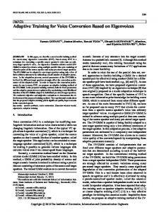
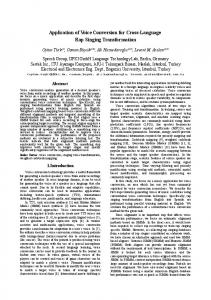
Figure 1: SAE, SJAE, and DNN architectures During AE training in its simplest form, weights are optimized to minimize the average reconstruction error E = kx x ˆk2 . However, this training schema may not result in extracting useful features since it can lead to over-fitting. One strategy to avoid this phenomenon is to use a form of regularizations, such as the dropout method which randomly zeroes certain input components [18]. Additionally, a deeper AE architecture and accompanying more effective encoding can be achieved by training multiple AEs layer-by-layer and stacking them [19], using the following approach: The first AE is trained on the input. The input is then encoded and passed to the next AE, which is trained on these encoded values, and so on. Finally, the AEs are stacked together to form a stacked-AE (SAE).

2.3. Joint-Autoencoder We can adapt SAEs to best-perform on the source and target speaker, respectively, using two separate SAEs. However, the source encodings and the target encodings are likely to be uncorrelated. Hence we will need another mapping to map the encodings from the source speaker to the encodings of the target speaker [9, 17]. To maximize the similarity of the encoding values, and relieve the need for the extra mapping, we propose a Joint-Autoencoder (JAE) , i. e. hx = fhid (Wx + bhid ), hy = fhid (Vy + chid ),

(3)

D RA FT

x ˆ = fvis (W> hx + bvis ),

mapped by an ANN [17]. Config-4 includes the creation of a SJAE prior to back-propagation. The additional effect of pretraining the SJAE using similar speaker’s data (“SJAE-20”) is explored in Config-5. Finally, Config-6 is identical to Config-5 except we use only one frame. Comparing 1 and 6 shows the effects of semi-supervised learning versus supervised learning. Comparing 5 and 6 shows the effects of considering 15 frames versus only one frame. Comparing 2 and 5 shows the effect of pre-training using similar speakers. For configurations involving the SAE, we randomly selected 80% of the 630 speakers for training, 10% for validation and 10% for testing purposes. We trained various SAE architectures, using dropout with a corruption level of 0.1. All activation functions were tangent hyperbolic, except for the first-level AE, for which we selected g of Equation 3 to be linear. For Configurations 5 and 6, we searched for the 10 most similar speakers among the TIMIT speakers in the training partition, for both source and target speakers, respectively, using a standard speaker identification approach [26]. Two parallel sentences for each of the 10 “similar” speaker-pairs were available. The utterances were time-aligned using DTW, and then used to pre-train the SJAE.

y ˆ = fvis (V> hy + cvis ),

where V and c are the weights and biases responsible for reconstructing the target. We modify the cost function to include the mean squared error between the encodings: E = kx

x ˆk2 + ky

y ˆk2 + ↵ khx

hy k 2 .

(4)

Similar to AEs, JAEs can also be stacked together for the purposes of initializing a DNN. The JAEs however are speakerdependent, thus help the network training by starting from an even better initialized state. The first JAE is trained on source and target parameters, which are then encoded. The same process is done for the encoded source and target features to train the second JAE. The process is iterated until the desired number of JAEs are trained, at which point the encoding parts of the source autoencoder are appended together to form the encoding part of the stacked-joint-autoencoder (SJAE), and the decoding parts of the target autoencoder are stacked together to form the decoding part of the SJAE. The final DNN is initialized by appending the encoding and the decoding parts together. The proposed architecture has the advantage of initializing all the DNN layers independently of each other, helping the backpropagation start from a better initial state, thus addressing the vanishing gradient problem [20]. The proposed DNN training scheme is shown in Figure 1.

3. Experiment

3.1. Training

For the VC experiment, we used the CMU Arctic corpus [21]. We considered two inter-gender conversions, namely CLB!SLT (females), and RMS!BDL (males). From each speaker, we selected 100, 50, and 5 parallel training, test, and validation sentences, respectively. Sentences were time-aligned using dynamic time warping (DTW). As speech features, we used 24th order MCEPs (excluding the 0th coefficient), extracted using the SPTK toolkit with 10 ms frame shift and 25 ms frame size [22]. Based on a study of phone recognition on the TIMIT database [23], we chose to model 15 frames (the current frame plus 7 preceding and following frames) [24] for multi-frame experiments, for a total of 15⇥24=360 features per frame. We considered several system configurations, listed in Table 1. Config-0 represents a classic baseline method [25]. Config-1 is designed to evaluate the efficacy of a DNN without prior unsupervised training [3]. Config-2 explores the effectiveness of unsupervised pre-training using the SAE and considering multiple frames. The key idea behind Config-3 is to regard the SAE as a feature extractor, whose features are subsequently

3.2. Objective Evaluation

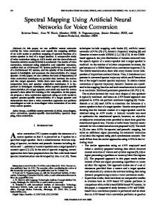
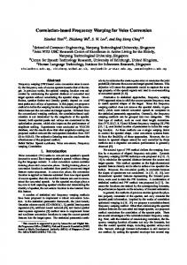
For Configurations 1–6, we selected the best DNN architectures from multiple 4-layer architectures with different hidden layer sizes; for example, the final DNN of Configuration 5 has layer sizes [360N 1000N 500N 1000N 360L], where N and L stand for non-linear and linear activation function. The corresponding SAE of this DNN resulted in a mel-cepstral distortion between original and reconstructed features of 0.99 dB. The average reconstruction error of SAEs on CLB and SLT was 1.14 dB. We trained the CLB!SLT mapping using different number of sentences, ranging from 1 to 100. The results are shown in Table 2. As an upper bound, we calculated the average distortion between the original source and target speakers’ spectral envelopes to be 7.76 dB. As a lower bound, past experiences have shown that different renditions of the same sentence by the same speaker result in an average distortion of approximately 5.30 dB. The results are shown in Table 2. 3.3. Subjective Evaluation

To subjectively evaluate voice conversion performance, we performed two perceptual tests: the first test measured speech quality and the second test measured conversion accuracy (also referred to as speaker similarity between conversion and target). The listening experiments were carried out using Amazon Mechanical Turk [27], with participants who had approval ratings of at least 90% and were located in North America. Both perceptual tests used three trivial-to-judge sentence pairs, added to the experiment to filter out any unreliable listeners. We used two training sets for subjective evaluation: a large set, which included 100 training utterances, and a small set, which included 5 training utterances. 3.3.1. Speech Quality Test To evaluate the speech quality of the converted utterances, we conducted a comparative mean opinion score (CMOS) test. In this test, listeners heard two utterances A and B with the same content and the same speaker but in two different conditions, and are then asked to indicate wether they thought B was better or worse than A, using a five-point scale comprised of +2 (much

# 0 1 2 3 4 5 6

frames 1 1 15 15 15 15 1

SAE

X X X X X

ANN

SJAE-20

SJAE

X X X

X X X

map GMM DNN DNN DNN DNN DNN DNN

0L

6L *

6L

0S

6S *

6S

6S

1S

1L

1L

5L

1S

1S

5S

* 1L

* 1L

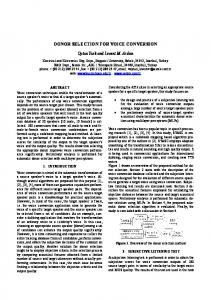
Table 1: System configurations Figure 3: Speech quality, with asterisks showing significantly better configuration. The digit represents the config number and S/L represents small and large number of training utterances.

Mel-cepstral distortion (dB)

D RA FT

config 0 config 1 config 2 config 3 config 4 config 5 config 6

8

0.4

large small

7

0.2

6

0

Config 0

100

101 Number of parallel training utterances

102

Figure 2: Mel-cepstral distortion between converted and target features (in dB).

better), +1 (somewhat better), 0 (same), -1 (somewhat worse), -2 (much worse). . The experiment was administered to 20 listeners with each listener judging 40 sentence pairs. Listeners’ preference scores are shown in Figure 3. For both the large and small sets, pre-trained DNNs performed better than the baseline DNN (t-tests for both 6L vs. 1L and 6S vs. 1S were significant). In addition, the baseline DNN trained with the large set performed significantly better, compared to all DNNs trained with the small set (1L vs. 6S and 1L vs. 1S). 3.3.2. Conversion Accuracy Test To evaluate the conversion accuracy of the converted utterances, we conducted a same-different speaker similarity test [28]. In this test, listeners heard two stimuli A and B with different content, and were then asked to indicate wether they thought that A and B were spoken by the same, or by two different speakers, using a five-point scale comprised of +2 (definitely same), +1 (probably same), 0 (unsure), -1 (probably different), and -2 (definitely different). One of the stimuli in each pair was created by one of the four mapping methods, and the other stimulus was a purely MCEP-vocoded condition, used as the reference speaker. Half of all pairs were created with the reference speaker identical to the target speaker of the conversion (the “same” condition); the other half were created with the reference speaker being of the same gender, but not identical to the target speaker of the conversion (the “different” condition). The

Config 1

Config 5

Config 6

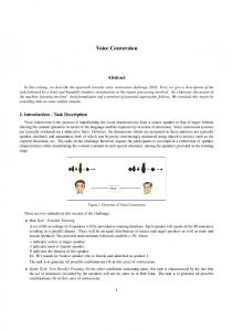
Figure 4: Conversion accuracy, with white and black bars representing the large and small training set, respectively.

experiment was administered to 50 listeners, with each listener judging 48 sentence pairs. Listeners’ average response scores (scores in the “different” conditions were multiplied by 1) are shown in Figure 4. We did not find any difference between the baseline GMM and the baseline DNN. For both large and small sets, a significant difference was found between the baseline DNN and the pretrained DNNs using both single and multiple frames. We did not find any significant difference between single-frame and multiple-frame pre-trained DNNs. Finally, we did not find any significant difference between the pre-trained DNN trained on the small set and the baseline DNN trained on the large set. The statistical tests in this subsection were performed using the Mann-Whitney test [29].

4. Conclusion In this study, we proposed a novel Stacked-Joint-Autoencoder architecture, which aims to find a common encoding of parallel source and target features. We also proposed to train the SJAE using unrelated speakers that are similar to the source and target speaker, instead of using only the source and target speakers. We pre-trained the DNN using the SJAE and further fine-tuned the network. We trained two speaker conversions and compared several system configurations objectively and subjectively while varying the number of available training sentences. The subjective and objective results showed that the semi-supervised learning scheme helps the training of the DNN significantly. We also found significant improvements in both speech quality and conversion accuracy.

5. References [1] S. H. Mohammadi and A. Kain, “Transmutative voice conversion,” in Acoustics, Speech and Signal Processing (ICASSP), 2013 IEEE International Conference on. IEEE, 2013, pp. 6920–6924. [2] D. Erro, A. Moreno, and A. Bonafonte, “Inca algorithm for training voice conversion systems from nonparallel corpora,” Audio, Speech, and Language Processing, IEEE Transactions on, vol. 18, no. 5, pp. 944–953, 2010.

[16] D. Erhan, Y. Bengio, A. Courville, P. A. Manzagol, P. Vincent, and S. Bengio, “Why does unsupervised pre-training help deep learning?” The Journal of Machine Learning Research, vol. 11, pp. 625–660, 2010. [17] S. H. Mohammadi and A. Kain, “Voice conversion using deep neural networks with speaker-independent pretraining,” in Spoken Language Technology (SLT). IEEE, 2014. [18] N. Srivastava, G. Hinton, A. Krizhevsky, I. Sutskever, and R. Salakhutdinov, “Dropout: A simple way to prevent neural networks from overfitting,” The Journal of Machine Learning Research, vol. 15, no. 1, pp. 1929–1958, 2014.

D RA FT

[3] S. Desai, A. W. Black, B. Yegnanarayana, and K. Prahallad, “Spectral mapping using artificial neural networks for voice conversion,” Audio, Speech, and Language Processing, IEEE Transactions on, vol. 18, no. 5, pp. 954–964, 2010.

[15] L.-H. Chen, Z.-H. Ling, and L.-R. Dai, “Voice conversion using generative trained deep neural networks with multiple frame spectral envelopes,” in Proc. Interspeech, 2014.

[4] E. Azarov, M. Vashkevich, D. Likhachov, and A. Petrovsky, “Real-time voice conversion using artificial neural networks with rectified linear units,” in INTERSPEECH, 2013, pp. 1032–1036. [5] L. J. Liu, L. H. Chen, Z. H. Ling, and L. R. Dai, “Using bidirectional associative memories for joint spectral envelope modeling in voice conversion,” in Acoustics, Speech and Signal Processing (ICASSP), 2014 IEEE International Conference on. IEEE, 2014. [6] J. Nirmal, M. Zaveri, S. Patnaik, and P. Kachare, “Voice conversion using general regression neural network,” Applied Soft Computing, vol. 24, pp. 1–12, 2014.

[7] L. H. Chen, Z. H. Ling, Y. Song, and L. R. Dai, “Joint spectral distribution modeling using restricted boltzmann machines for voice conversion,” in INTERSPEECH, 2013.

[8] Z. Wu, E. S. Chng, and H. Li, “Conditional restricted boltzmann machine for voice conversion,” in Signal and Information Processing (ChinaSIP), 2013 IEEE China Summit & International Conference on. IEEE, 2013, pp. 104–108. [9] T. Nakashika, R. Takashima, T. Takiguchi, and Y. Ariki, “Voice conversion in high-order eigen space using deep belief nets,” in INTERSPEECH, 2013, pp. 369–372.

[10] L.-H. Chen, Z.-H. Ling, L.-J. Liu, and L.-R. Dai, “Voice conversion using deep neural networks with layer-wise generative training,” IEEE/ACM Transactions on Audio, Speech and Language Processing (TASLP), vol. 22, no. 12, pp. 1859–1872, 2014. [11] H. Duxans, A. Bonafonte, A. Kain, and J. Van Santen, “Including dynamic and phonetic information in voice conversion systems,” in Proc. of the ICSLP’04, 2004.

[12] T. Toda, A. W. Black, and K. Tokuda, “Voice conversion based on maximum-likelihood estimation of spectral parameter trajectory,” IEEE Transactions on Audio, Speech, and Language Processing Journal, vol. 15, no. 8, pp. 2222–2235, November 2007. [13] F.-L. Xie, Y. Qian, Y. Fan, F. K. Soong, and H. Li, “Sequence error (se) minimization training of neural network for voice conversion,” in Proc. Interspeech, 2014. [14] T. Nakashika, T. Takiguchi, and Y. Ariki, “Voice conversion using rnn pre-trained by recurrent temporal restricted boltzmann machines,” Audio, Speech, and Language Processing, IEEE/ACM Transactions on, vol. 23, no. 3, pp. 580–587, March 2015.

[19] P. Vincent, H. Larochelle, I. Lajoie, Y. Bengio, and P.A. Manzagol, “Stacked denoising autoencoders: Learning useful representations in a deep network with a local denoising criterion,” The Journal of Machine Learning Research, vol. 11, pp. 3371–3408, 2010. [20] X. Glorot and Y. Bengio, “Understanding the difficulty of training deep feedforward neural networks,” in International conference on artificial intelligence and statistics, 2010, pp. 249–256. [21] J. Kominek and A. W. Black, “The cmu arctic speech databases,” in Fifth ISCA Workshop on Speech Synthesis, 2004. [22] T. Toda, A. W. Black, and K. Tokuda, “Voice conversion based on maximum-likelihood estimation of spectral parameter trajectory,” Audio, Speech, and Language Processing, IEEE Transactions on, vol. 15, no. 8, pp. 2222– 2235, 2007. [23] J. S. Garofolo, L. F. Lamel, W. M. Fisher, J. G. Fiscus, and D. S. Pallett, “Darpa timit acoustic-phonetic continous speech corpus cd-rom. nist speech disc 1-1.1,” NASA STI/Recon Technical Report N, vol. 93, p. 27403, 1993. [24] A. R. Mohamed, G. E. Dahl, and G. Hinton, “Acoustic modeling using deep belief networks,” Audio, Speech, and Language Processing, IEEE Transactions on, vol. 20, no. 1, pp. 14–22, 2012. [25] A. Kain and M. Macon, “Spectral voice conversion for text-to-speech synthesis,” in Proceedings of ICASSP, vol. 1, May 1998, pp. 285–299. [26] D. A. Reynolds and R. C. Rose, “Robust test-independent speaker identification using gaussian mixture models,” IEEE Transactions on Speech and Audio Processing, vol. 3, pp. 72–83, 1995. [27] M. Buhrmester, T. Kwang, and S. D. Gosling, “Amazon’s mechanical turk — a new source of inexpensive, yet highquality, data?” Perspectives on Psychological Science, vol. 6, no. 1, pp. 3–5, January 2011. [28] A. Kain, “High Resolution Voice Transformation,” Ph.D. dissertation, OGI School of Science & Engineering at Oregon Health & Science University, 2001. [29] H. B. Mann and D. R. Whitney, “On a test of whether one of two random variables is stochastically larger than the other,” The annals of mathematical statistics, pp. 50–60, 1947.