SEMIDEFINITE PROGRAMMING RELAXATIONS for SET ... - CiteSeerX

SEMIDEFINITE PROGRAMMING RELAXATIONS for SET PARTITIONING PROBLEMS  y

Henry Wolkowicz, and Qing Zhao

z

October 14, 1996 University of Waterloo CORR Report 96-??

Abstract

We present a relaxation for the set partitioning problem that combines the standard linear programming relaxation with a semide nite programming relaxation. We include numerical results that illustrate the strength and eciency of this relaxation.

Contents

1 INTRODUCTION

2

2 SDP RELAXATION 3 NUMERICAL TESTS 4 SDP RELAXATION FOR LARGE SPARSE PROBLEMS

3 8 8

1.1 Background . . . . . . . . . . . . . . . . . . . . . . . . . . . . . . . . . . . . . . .

2

4.1 An SDP Relaxation with Block Structure . . . . . . . . . . . . . . . . . . . . . . 8 4.2 An Infeasible Primal-Dual Interior-Point Method . . . . . . . . . . . . . . . . . . 13 4.3 Preliminary Numerical Tests and Future Work . . . . . . . . . . . . . . . . . . . 15

A APPENDIX-Notation

16

 This report is available by anonymous ftp at orion.uwaterloo.ca in the directory pub/henry/reports; or over WWW with URL ftp://orion.uwaterloo.ca/pub/henry/reports/ABSTRACTS.html y University of Waterloo, Department of Combinatorics and Optimization, Faculty of Mathematics, Waterloo, Ontario, N2L 3G1 Canada

1 INTRODUCTION We present a relaxation for the set partitioning problem (denoted SP) that combines the standard linear programming relaxation with a semide nite programming (denoted SDP) relaxation. We include numerical results that illustrate the strength and eciency of this relaxation.

1.1 Background

The set partitioning problem, SP, can be described as follows. Suppose we are given a set M with m elements; and let

M = fMj : j 2 N := f1; 2; : : :; ngg be a given collection of subsets of M such that the union contains M , i.e. [j 2N Mj = M . For each Mj , there is an associated cost cj  0. We want to nd a subset F of the index set N such that: 1. the union still contains M , [j 2F Mj = M ; 2. the sets are pairwise disjoint, Mk \ Mj = ; for k 6= j 2 F ; 3. and the sum of the costs Pi2F cj is minimized. Let A = (aij ) be the m  n matrix with

aij =

(

1 if element i 2 Mj 0 otherwise:

This matrix A is called the incidence matrix of the collection M; each column of A is the indicator vector for the set Mj : Each subset F  N; for which the collection of sets fMj ; j 2 F g satis es conditions 1 and 2, is called a set partition of the set M . For a given set partition, we let x 2 f0; 1gn be de ned by ( if j 2 F xj = 01 otherwise :

Such an x represents the set partition. The set partitioning problem can now be formulated as the following 0-1 integer programming problem  := min ct x (SP ) subject to Ax = e x 2 f0; 1gn; where e is the vector of ones. Without loss generality, we assume that the feasible set of (SP) is nonempty and that A has full row rank. For each i 2 f1; 2; : : :; mg, we let

ai := (ai1 ; ai2; : : :; ain): The i-th constraint, ai x = 1; guarantees that the i-th element is in exactly one set. 2

The set partitioning problem has been extensively investigated because of its special structure and its numerous practical applications. The best known application is airline crew scheduling, see e.g. the recent reference [14]. Other applications include: truck scheduling; bus scheduling; facility location; circuit design and capital investment. (For applications and algorithms see e.g Gar nkel and Nemhauser [11], Marsten [16], Balas and Padberg [4], Balas [3], Nemhauser and Weber [17], Fisher and Kedia [10] Chan and Yano [6] and Homan and Padberg [15].) Since the set partitioning problem is well-known to be NP-hard, many current approaches focus on nding a \near optimal" solution using various heuristic techniques. A natural candidate for generating a lower bound is the linear programming relaxation. LP := min ct x (SPLP ) subject to Ax = e x  0: To improve the approximate solution for (SP), one can use cutting planes and/or branch-andbound techniques in conjunction with various bound improvement techniques. In addition, various heuristics have been tried. (See Chu and Beasley [8] for a literature survey on exact and heuristic algorithms for (SP).) We include the following related papers in the bibliography [1, 2, 5, 12, 13, 18] The latex bib le can be obtained over WWW or with anonymous ftp using URL: ftp://orion.uwaterloo.ca/pub/h In this paper, we develop an SDP relaxation for the set partitioning problem. Our approach is similar to that in [21, 22, 20]; i.e.: we derive a semide nite relaxation from the dual of the dual of a quadratic constrained quadratic program formulation of (SP); we employ a \gangster operator" to eciently model the 0-1 constraints in the relaxation; we project the feasible set onto the minimal face of the semide nite cone in order to guarantee a constraint quali cation; and we apply a primal-dual interior-point (p-d i-p) algorithm with an incomplete conjugate gradient method to solve the SDP relaxation. In addition, we combine the SDP relaxation with the standard LP relaxation and take advantage of block structures in the data.

2 SDP RELAXATION To derive an SDP relaxation for SP, we reformulate the 0-1 integer programming model as a quadratically constrained quadratic programming problem. Since the variables xi are restricted to 0-1, we have xi = x2i , i.e. x = x  x; where  denotes the Hadamard, or elementwise, product. In addition, since ai x = 1; for each i 2 f1; : : :; mg, we have fk 6= j; aik = 1; aij = 1g ) xk xj = 0: (2.1) Therefore (SP) is equivalent to the following.  = min ct(x  x) subject to A(x  x) = e (SPQP ) (ai x ? 1)2 = 0; for i 2 f1; 2; : : :; mg (x  x) ? x = 0 xk xj = 0; if k 6= j; and aik = aij = 1; for some i: 3

By adding a scalar x0 , we can eliminate the linear terms (homogenize) in the existing constraints of the above problem.  = min ct(x  x) subject to A(x  x) = e (?1; ai)(x0; xt)t(x0 ; xt)(?1; ai)t = 0; for i 2 f1; 2; : : :; mg (SPQPH ) (x  x) ? x0 x = 0 xk xj = 0; if k 6= j; and aik = aij = 1; for some i x20 = 1: We now replace the quadratic terms with a matrix, i.e.we replace the rank one matrix (x0 ; xt)t(x0; xt) by the positive semide nite matrix Y  0 with Y 2 Sn+1 , the space of n + 1  n + 1 symmetric matrices. We get the following SDP relaxation. SDP := min trace CY subject to trace (Diag([0; ai])Y ) = 1; i = 1; : : :; m (?1; ai )Y (?1; ai)t = 0; i = 1; : : :; m arrow (Y ) = e0 (PSDP ) GJ (Y ) = 0 Y00 = 1 Y  0;     where C = Diag ( 0; ct ) is the diagonal matrix formed from the vector 0; ct , and the operator GJ is a gangster operator, i.e. GJ : Sn+1 ! Sn+1 shoots \holes" (or zeros) in a matrix. The ij component is de ned as ( (i; j ) or (j; i) 2 J (GJ (Y ))ij := Y0 ij ifotherwise. (2.2) where the set J := f(k; j ) : if k 6= j and aik = aij = 1 for some ig; the gangster operator is self-adjoint, GJ = GJ . The arrow operator, acting on the (n +1)  (n +1) matrix Y; is de ned as arrow (Y ) := diag (Y ) ? (0; (Y0;1:n2 )t; (2.3) where Y0;1:n2 is the vector formed from the last n2 components of the rst, or 0, row of Y and diag denotes the vector formed from the diagonal elements; e0 is the rst unit vector. The arrow constraint represents the 0,1 constraints by guaranteeing that the diagonal and 0-th row (or column) are identical; the gangster operator constraint represents the constraints in (2.1); and, nally, the assignment constraints Ax = e are represented by the rst two sets of constraints in (PSDP). De ne the m  (n + 1) assignment constraint matrix T := [?e; A]: Each feasible Y satis es Y  0 and (?1; ai)Y (?1; ai)t = 0; i = 1; : : :; m: 4

Therefore the range space and null space satisfy

R(T t)  N (Y ) or alternatively R(Y )  N (T ): Now let the null space of T be spanned by the columns of a (n + 1)  (n ? m + 1) matrix V , i.e.

let

N (T ) = R(V ): This implies that Y = V ZV t for some Z = Z t  0; i.e. we are able to express each feasible Y

as V ZV t . In order to solve large scale problems, a sparse representation of the null space of T is useful. We use a simple technique, called Wolfe's variable-reduction technique [19]. (For a \sparsest" representation, see e.g. [9].) Without loss generality, we assume that

T = [TB ; TN ]; where TB is a m  m matrix with full rank and TN is a m  (n ? m + 1) matrix. Then, the matrix " ?1 # V = ?ITB TN n?m+1

satis es N (T ) = R(V ): We now take a look at the following interesting properties of the matrix V ZV t .

Lemma 2.1 For any arbitrary (n ? m + 1)  (n ? m + 1) symmetric matrix 2 3 Z Z : : : Z n?m 66 Z Z : : : Z n?m 777 6 Z = 6 .. .. .. ... 75 ; 4 . . . 00

01

0(

)

10

11

1(

)

Z(n?m)0 Z(n?m)1 : : : Z(n?m)(n?m)

let Y = V ZV t and write Y as

2 66 Y = 66 4

3

Y00 Y01 : : : Y0n Y10 Y11 : : : Y1n 777 .. .

.. .

...

.. 7 : . 5

Yn0 Yn1 : : : Ynn

Then: a)

ai Y1:n;0 = Y00; for i = 1; : : :; m; b)

Y0j = ai Y1:n;j ; for i = 1; : : :; m; j = 1; : : :; n: 5

Proof. Since

TY = TV ZV t = 0; we have, (?1; ai)Y = 0, for each 1  i  m.

2

This shows that the rst two sets of constraints are redundant. Before we write our nal SDP relaxation, we present another lemma which helps get rid of more redundant constraints. Lemma 2.2 Let Y = V ZV t with Y00 = 1: Then

GJ (Y ) = 0 ) arrow (Y ) = e : Proof. Suppose Y = V ZV t and GJ (Y ) = 0: Let j 2 f1; 2; : : :; ng. Then there exists i 2 f1; 2; : : :; mg such that aij = 1: By Lemma 2.1, we have (ai ; : : :; ain)Y n;j = Y j : This implies that X 0

1

Yjj +

k k6=j;aik =1

1:

0

Ykj = Y0j :

From the de nition of the gangster operator, we have

X

k k6=j;aik =1

Ykj = 0:

Therefore Yjj = Y0j :

2

Now replacing Y by V ZV t in (PSDP) and getting rid of the redundant constraints, we have the following nal SDP relaxation for SP. We let J 0 = J [ f(0; 0)g. (PSDPF )

SDP =

min trace V t CV Z subject to GJ 0 (V ZV t ) = E00 Z  0;

where Z 2 Sn?m+1 and C = Diag (0; ct): The dual is (DSDPF )

max W00 subject to V t GJ0 (W )V  V t CV:

From Lemma 2.1 and Lemma 2.2, we can immediately derive the following. Theorem 2.1 Let Z be any feasible solution of (PSDPF). Then (diag (V ZV t))1:n (the last n diagonal elements of the matrix V ZV t ), is a feasible solution of the linear programming relaxation (SPLP).

Proof. Let Z satisfy the hypothesis and Y = V ZV t. Then GJ (Y ) = E and Yjj  0; for i 2 f1; : : :; ng: 0

6

00

From Lemma 2.1 and Lemma 2.2, we have Y:;0 = diag (Y ) and Y00 = 1, and thus for each i 2 f1; : : :; mg, ai(Y11; : : :; Ynn )t = aiY0tj = Y00 = 1:

2

Based on the theorem above and the fact that the objective value of the SDP relaxation is (0; ct)diag (V ZV t), the following corollary follows. Corollary 2.1 The lower bound given by the SDP relaxation (PSDPF ) is greater than or equal to the one given by the LP relaxation, i.e. SDP  LP . In addition, we now see that there is no duality gap between (PSDPF) and (DSDPF).

Theorem 2.2 Problem (DSDPF) is strictly feasible. Proof. From Lemma 2.2, we have GJ (V ZV t) = 0 ) arrow (V ZV t) = 0: 0

Therefore

N (GJ 0 (V
V t))  N (arrow(V
V t)):

In other words, their adjoint operators satisfy R(V tArrow (
)V )  R(V tGJ 0 (
)V ): Therfore for y = ?e 2 Rn+1 , there exists W such that V tArrow (?en)V = V t GJ 0 (W )V and, by using Schur complements, we see that V tGJ 0 (?E00 + W )V = V t(?E00 ? Arrow (en))V  0; for  big enough. Therefore (?E00 + W ) is strictly feasible for large enough :

2

From Theorem 2.2, we know that the dual problem satis es the Slater condition. Therefore, there is no duality gap between the primal problem (PSDPF) and the dual problem (DSDPF) and, moreover, the primal optimal value is attained. However, the primal problem may not be strictly feasible.

Example 2.1 Consider SP with constraints

x1 =1 x1 +x2 +x3 +x4 = 1 x1 ; x2; x3; x4  0: Observe that the feasible set is a singleton (1; 0; 0; 0)t. Note that for this problem n = 4 and m = 2, so V is a 5  3 matrix. Thus, for any feasible solution of its nal SDP relaxation Z 2 P3, the diagonal of V ZV t is (1; 1; 0; 0; 0)t. This means that rank (V ZV t )  2, which implies that rank (Z )  2. Therefore, the nal SDP relaxation is not strictly feasible. 7

small01 small02 small03 small04 small05 tiny04 tiny01 tiny05

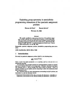
nrow ncol nzero LP SDP 14 34 108 1864 1864* 16 46 139 2259 2259* 27 97 234 17327 18324 33 192 584 4503 4503* 44 277 770 21706 21706* 6 27 72 1035 1091 3 6 9 17.5 25.00 7 35 70 1215 1257 Table 1: Numerical Results

3 NUMERICAL TESTS The algorithm (a p-d i-p approach) we use to solve the SDP relaxation is very similar to the one in [21, 22, 20] for the quadratic assignment and graph partitioning problems. An incomplete conjugate gradient method is used to solve the large Newton equations that arise at each iteration of the algorithm. As we have seen from the geometrical discussion above, the algorithm may have to deal with those problems whose primal SDP relaxation are not strictly feasible and whose dual SDP relaxation can not attain their optimal value. Since the main purpose of our algorithm is to nd good lower bounds, we apply an infeasible primal-dual interior-point algorithm. Because the dual problem is strictly feasible and only has inequality constraints, the linesearch can easily maintain dual feasibility. Therefore, a lower bound can always be obtained from the dual objective value. The purpose of our numerical tests is to illustrate that the lower bound given by our algorithm for the SDP relaxation is better than the one given by LP relaxation. In addition, after solving the relaxation, the diagonal of the matrix Y from the SDP relaxation satis es the constraints of the linear programming relaxation. Our numerical tests for small problems are based on real data for bus scheduling ????ref!!!??? problems. The results are summarized in Table 1. The columns under nrow, ncol and nzero are for the number of rows, columns and nonzero elements, respectively. The last two columns show the lower bounds by LP and SDP relaxations, respectively. A lower bounds marked with a star means that the lower bound is equal to the optimal objective value.

4 SDP RELAXATION FOR LARGE SPARSE PROBLEMS 4.1 An SDP Relaxation with Block Structure

As we see from the introduction, the set partitioning problems are usually derived from real world problems such as scheduling problems. These problems can be of very large size (> 10; 000) and very sparse. 8

Currently, an approximate solution for a large size set partitioning problem can be obtained by solving a corresponding large sparse linear programming relaxation and the information from the primal and dual optimal solutions are used to decide which columns, or sets Mj , should be chosen for the partition. Since the diagonal of an SDP solution is a feasible solution of the LP relaxation, we expect that this solution can help in making the choices. On the other hand, it is hard to solve SDP problem of large size, e.g. over 10,000. In order to make SDP relaxation more competitive with LP to solve the large sparse problem, we have to nd a way to exploit the sparsity of the set partitioning problem. In this section, we relax part of the variables of the set partitioning by SDP, while we treat the others with an LP relaxation. Consider a large sparse set partitioning problem (SPL)

 =

min ct x subject to Ax = e x 2 f0; 1gn:

By permuting the rows and columns of A, we can rewrite A as

2 66 6 A = 66 64

F1 0 .. . 0 G1

::: ::: ... ::: :::

0 F2 .. . 0 G2

0 0 .. . Fk Gk

0 0 .. . 0 H

3 77 77 77 ; 5

(4.4)

where for each i 2 f1; : : :; kg, Fi is mi  ni , Gi is mG  ni ; H is mG  nH ; and

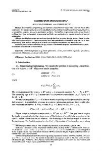
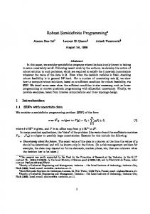
m1 + : : : + mk + mG = m; n1 + : : : + nk + nH = n: The sparsity pattern of the matrix A is illustrated in Figure 2. Corresponding to each submatrix Fi , i 2 f1; : : :; kg, we de ne

xBi = (x1Bi ; : : :; xnBii )t and xN = (x1N ; : : :; xnNH )t such that Similarly, we de ne such that



x = xB1 : : :xBk xN

t

:

cBi = (c1Bi ; : : :; cnBii )t; and cN = (c1N ; : : :; cnNH )t





For each i 2 f1; : : :; kg, we write

2 Fi = 64

c = cB1 : : :cBk cN : Fi1 .. . Fimi

3 2 75 = 66 4

Fi11 .. . m Fi i 1 9

3

: : : Fi1ni 7 . . . ... 7 : 5 m n i i : : : Fi

Figure 1: Sparsity Pattern of Matrix A

Figure 2: Sparsity Pattern

10

Similarly, for each i 2 f1; : : :; kg, we write

2 Gi = 64

2 H = 64

2 G1i 3 6 G11 i .. 75 = 6 .. . 4 m. 1 m G Gi Gi G

H 1 3 2 H 11 .. 75 = 64 .. . . H mG H mG 1 and de ne an index sets for gangster operators

(

3

: : : Gi1ni 7 .. 7 ; ... . 5 m : : : Gi Gni

: : : H 1nH 3 .. 75 : ... . : : : H mGnH

)

jp = F jq = 1 or i : Ji := (p; q) : p < q for some j FGijp = jq = 1 G i i

We rewrite (SPLP ) as

 =

Pk ct x + ct x min i=1 Bi Bi N N subject to Fi xBi = emi ; i 2 f1; : : :; kg G1 xB1 + : : : + Gk xBk + HxN = emG xB1 ; : : :; xBk ; xN 2 f0; 1gn:

An equivalent quadratically constrained quadratic programming formulation can then be expressed as follows

 =

Pk ct x  x + ct x  x min i=1 Bi Bi Bi N N N subject to Fi xBi  xBi = emi ; (Fij xBi ? 1)2 = 0; for j 2 f1; 2; : : :; mig; xBi  xBi ? xBi = 0; xpBi xqBi = 0; for any pair (p; q) 2 Ji ; for i 2 f1; : : :; kg G1xB1  xB1 + : : : + Gk xBk  xBk + HxN  xN = e:

By adding, for each i 2 f1; : : :; kg, a scalar x0Bi , we homogenize the above problem as follows

 =

P

k ct x  x + ct x  x min i=1 Bi Bi Bi N N N subject to Fi xBi  xBi = emi ; (?1; Fij )(x0Bi ; xtBi )t(x0Bi ; xtBi )(?1; Fij )t = 0; for j 2 f1; 2; : : :; mi g; xBi  xBi ? x0Bi xBi = 0; (x0Bi )2 = 1; xpBi xqBi = 0; for any pair (p; q) 2 Ji ; for i 2 f1; : : :; kg G1xB1  xB1 + : : : + Gk xBk  xBk + HxN  xN = e:

11

In the above quadratically constrained quadratic programming, we replace the rank-one matrix (x0Bi ; xtBi )t(x0Bi ; xtBi ) by the matrix Yi for each i 2 f1; : : :; kg, and also XN XNt by YN . Then we obtain an SDP relaxation as follows Pk ct (diag (Y )) + ct diag (Y ) LR := min i 1:ni N i=1 Bi N subject to Fi (diag (Yi ))1:ni = emi ; (?1; Fij )Yi (?1; Fij )t = 0; for j 2 f1; 2; : : :; mig; arrow (Yi ) = 0; (Yi )00 = 1; GJi (Yi) = 0; for 1; : : :; kg Pk i G2 f(diag (Yi ))1:ni + H diag (YN ) = e; i=1 i Y1  0; : : :; Yk  0; YN  0; where Yi 2 Pni +1 for i 2 f1; : : :; kg and YN 2 PnH . Since the coecient matrices for YN are all diagonal, we can always write YN = Diag (x), where x 2 RnH ; x  0. For each i 2 f1; : : :; kg, we de ne an operator Ai : Pni +1 ! RmG such that Ai(Yi) := Gi(diag (Yi))1:ni : Then we have the following equivalent problem. Pk ct (diag (Y )) + ct x LR = min i 1:ni i=1 Bi N subject to Fi (diag (Yi ))1:ni = emi ; (?1; Fij )Yi (?1; Fij )t = 0; for j 2 f1; 2; : : :; mig; arrow (Yi ) = 0; (Yi )00 = 1; GJi (Yi) = 0; for kg Pk i A2 f(1Y; ): :+:;Hx = e; i=1 i i YB1  0; : : :; YBk  0; x  0: For each i 2 f1; : : :; kg, we construct a (ni + 1)  (ni ? mi + 1) matrix Vi such that the null space of [?emi ; Fi] is spanned by the columns of Vi . We follow the same procedure as that in the above section, i.e., for i 2 f1; : : :; kg, we replace Yi by ViXi Vit and get rid of the redundant constraints. We denote Ci := Diag (0; ctBi ). Note that ctBi (diag (Yi ))1:ni = trace (Diag (0; ctB)Yi ). Then we have the following nal SDP relaxation. Pk trace V tC V X + ct x LR = min Pki=1 A (V Xi V it)i+ iHx =N e subject to mG i=1 i i i i (LPSDPF ) GJi0 (Xi) = E00i ; for i 2 f1; : : :; kg X1  0; : : :; Xk  0; x  0; where, for i 2 f1; : : :; kg, Xi 2 Pni ?mi +1 and the operator GJi0 is a gangster operator with

)

(

jp F jq = 1 or i [ (0; 0): Ji := (p; q) : p < q for some j FGijp = jq = 1 = G i i 0

12

Observe that in the nal SDP relaxation (LSPRP ) there are semide nite matrix variables and nonnegative vector variables as well. Thus, we call the nal SDP relaxation a mixed LP-SDP relaxation. Its dual is PmG  + Pk (Y ) max i=1 i 00 i=1 i subject to Vit (Diag(0; tGi ) + Yi )Vi  Vit Ci Vi; Yi 2 SJi0 ; (LSPRD) for i 2 f1; : : :; kg H t  c; where for i 2 f1; : : :; kg, Yi and i are dual variables. For each feasible solution of (LSPRP ) (X1; : : :; Xk ; x), we construct a n  1 vector 0 1 BB y..1 CC y=B (4.5) B@ y.k CCA ; x where yi = (diag (ViXi )Vit )1:ni , for i = 1; : : :; k.PApplying the Theorem 2.1 to each block, we have Fi yi = emi for i = 1; : : :; k. Also note that ki=1 Gi yi + Hx = emG . Therefore, we have the following results. Theorem 4.1 Let (X1; : : :; Xk; x) be any feasible solution of (LSPRP ). Then the vector 1 0 (diag (V1X1 )V1t )1:n1

BB .. . BB @ (diag (VkXk )Vkt) x

nk

1:

CC CC A

is a feasible solution of the linear programming relaxation (SPLP ).

Based on the above theorem and the fact that Ci, for i = 1; : : :; k, are all diagonal matrices, the following corollary is straightforward. Corollary 4.1 The lower bound given by the SDP relaxation (LSPRP ) is great that or equal to the one given by the LP relaxation (SPLP ), i.e., LR  LP .

4.2 An Infeasible Primal-Dual Interior-Point Method

We rewrite the dual (LSPRD) by introducing a slack matrix Zi for each i 2 f1; : : :; kg and a slack vector z . PmG  + Pk (Y ) max i=1 i 00 i=1 i subject to Vit(Diag (0; tGi ) + Yi )Vi + Zi = Vit CiVi ; Yi 2 SJi0 ; (LSPRD) for i 2 f1; : : :; kg H t + z = c Z1  0; : : :; Zk  0; z  0: 13

The Karush-Kuhn-Tucker conditions of the dual log-barrier problem are

Pk A (V X V t) + Hx ? e i i i i mG i GJi0 (ViXiVit) ? E i for i 2 f1; : : :; kg H t + z ? c t Vi (Diag (0; tGi ) + Yi ? Ci )Vi + Zi for i 2 f1; : : :; kg z  x ? u Zi Xi ? I for i 2 f1; : : :; kg: =1

00

= FP0 = 0 = FPi 1 = 0; = FD0 = 0 = FDi = 0; 0 = FZX = 0 i = FZX = 0;

The rst two equations are primal feasibility conditions, while the third and fourth are the dual feasibility conditions and the last two takes cares of complimentary slackness for Xi and Zi and x and z, respectively. We solve this system of equations with a variant of Newton's method. We apply operators Ai and GJi0 to nonsymmetric matrices and then we linearize the above system as follows. Pk A (V X V t) + Hx = ?FP0 i=1 i i i i t GJi0 (ViXiVi ) = ?FPi 1 for i 2 f1; : : :; kg H t + z = ?FD0 (4.6) Vit(Diag (0; tGi ) + Yi ))Vi + Zi = ?FDi for i 2 f1; : : :; kg 0 z  x + z  x = ?FZX i Zi Xi + Zi Xi = ?FZX for i 2 f1; : : :; kg: From the third and fourth equations, we have, for i 2 f1; : : :; kg,

Zi = ?FDi ? Vit (Diag(0; tGi ) + Yi ))Vi and

z = ?FD0 ? H t: Substituting (4.7) and (4.8) into the last two equations, respectively, we have i + Z ?1 F i X + Z ?1 V t(Diag (0; tG ) + Y ))V X Xi = ?Zi?1 FZX i i i i i D i i i

and

(4.7) (4.8) (4.9)

0 x = ?z ?1  FZX + z ?1  FD0  x + z ?1  H t  x: (4.10) Substituting (4.9) and (4.10) into the rst two equations, we have the following nal normal equation. Pk A (V Z ?1V t(Diag (0; tG ) + Y )V X V t) i i i i i i=1 i i i i +Hz ?1  H t  x = ?FP0 + b0 (4.11) ? 1 t t t GJi0 (ViZi Vi (Diag(0;  Gi) + Yi )ViXiVi ) = ?FPi 1 + bi for i 2 f1; : : :; kg;

14

nrow ncol nzero LP SDP LP-SDP small03 27 97 234 17327 18324 18320 tiny04 6 27 72 1037 1091 1066 tiny01 3 6 9 17.5 25 25 tiny05 7 35 70 1215 1257 1248 Table 2: Numerical Results where

i ? Z ?1 F i Xi)V t ) + H (z ?1  F 0 ? z ?1  F 0  x); b0 = Pki=1 Ai (Vi(Zi?1 FZX i ZX D i D ? 1 i bi = GJi0 (Vi(Zi FZX ? Zi?1 FD1 Xi)Vit); for i 2 f1; : : :; kg: Denote the matrix representation of the left hand side of the normal equation by K. The matrix K has a very nice sparsity structure similar to A in Figure 1, where the width of the long narrow bar is mG which is much less than the size of the matrix. We solve the normal equation by a preconditioned conjugate gradient method. Let (Y1 ; : : :; Yk ; ) be the solution for the normal equation. By equations (4.7), (4.8), (4.9) and (4.10), we can obtain, for each i 2 f1; : : :; kg, Zi , zi,Xi and xi , respectively. Finally, by symmetrizing Xi, i.e.,  t Xi Xi +2(Xi ) ; we obtain a search direction. We then do a linesearch and update the current point. Based on the duality gap, we update  by using the following formula

Pk trace (Z X ) + ztx i i i  := 2( n ? m + mG + k ) : =1

4.3 Preliminary Numerical Tests and Future Work

In the previous subsections, we have developed an approach for solving problems with matrix structure (4.4). We did some preliminary numerical tests just to see how this SDP relaxation works for small problems. In our testing, we use the diagonal of the matrix representation K as the preconditioner. The infeasible primal-dual interior-point algorithm for the mixed LP-SDP relaxation is coded in C and Matlab. The results are summarized in Table 2. In Table 2, the columns under nrow, ncol and nzero are for the number of rows, columns and nonzero elements, respectively. The columns under LP and SDP show the lower bounds given by LP relaxation and SDP relaxation for a general dense problem, respectively, while the last column under LP-SDP shows the lower bounds given by our mixed LP-SDP relaxation. It remains to try and use the mixed LP-SDP relaxation to derive an approach to solve general large sparse set partitioning problems. To achieve this, we propose the following: 15

 to have the same matrix sparsity pattern as described for the mixed LP-SDP relaxation,

the matrix for the general problem need to be transformed into form like (4.4). This can be done by treating the 0-1 matrix A as an incidence matrix of a graph or netlist and applying graph partitioning and netlist partitioning techniques;  because of the nice sparsity structure as shown in Figure 5.1, more sophisticated incomplete factorization preconditioners can be used to improve the performance of primal-dual interior-point solvers, see e.g. [7].

A APPENDIX-Notation SP SDP M)

set partitioning problem semide nite programming problem given collection of subsets of M A = (aij ) incidence matrix of the collection M e the vector of ones ek the k-th unit vector ai the i-th row of incidence matrix A SPLP the linear programming relaxation for SP p-d i-p primal-dual interior-point (algorithm) BC the Hadamard product of B and C QR R ? Q is positive semide nite Sn the space of symmetric n  n matrices PSDP the semide nite relaxation primal problem Diag the diagonal matrix formed from the vector Pn or P the cone of positive semide nite matrices in Sn T [?e; A]; the assignment constraint matrix Slater CQ the Slater constraint quali cation; strict feasiblity p-d i-p primal-dual interior-point method G = (V ; E ) graph with node set V and edge set E cut edge an edge connecting nodes in dierent subsets of a partition 16

X = (xij ) partition matrix w(Ecut ) total weight of cut edges of the partition w(Ecut ) minimal total weight of cut edges over all partitions L Laplace matrix of the graph YX partition matrix lifted into higher dimensional matrix space m (m1; : : :; mk )t A B the Kronecker product of A and B vec (X ) the vector formed from the columns of the matrix A the n2 vector from the rst row of Y Y0;1:n2 diag the vector formed from the diagonal elements arrow the arrow operator diag (Y ) ? (0; (Y0;1:n2 )t GJ the gangster operator GJ shoots \holes" in a matrix R(B) range space of B N (B) null space of B J0 J 0 = J [ f(0; 0)g K
C K is a face of C relint relative interior diag (A) the vector formed from the diagonal of the matrix A Diag (v ) the diagonal matrix formed from the vector v En the matrix of ones in Sn Eij the ij unit matrix in Sn

References [1] J. ARABEYRE, J. FEARNLEY, F. STEIGER, and W. TEATHER. The airline crew scheduling problem: a survey. Transportation Science, 2:140{163, 1969. [2] E. BAKER and M. FISHER. Computational results for very large air crew scheduling problems. OMEGA, 9(6):613{618, 1981. [3] E. BALAS. Some valid inequalities for the set partitioning problems. Annals of Discrete Mathematics, 1:13{47, 1977. 17

[4] E. BALAS and M.W. PADBERG. Set partitioning: A survey. SIAM Review, 18:710{760, 1976. [5] J. BARUTT and T. HULL. Airline crew scheduling: aupercomputers and algorithms. SIAM News, 23(6), 1990. [6] T. J. CHAN and C. A. YANO. A multiplier adjustment approach for the set partitioning problem. Operations Research, 40:S40{S47, 1992. [7] PAULINA CHIN. Iterative Algorithm for Solving Linear Programming from Engineering Applications. PhD thesis, University of Waterloo, 1995. [8] P. C. CHU and J. E. BEASLEY. A genetic algorithm for the set partitioning problem. Technical report, Imperial College, The Management School, London, England, 1995. URL: http:/mscmga.ms.ic.ac.uk/pchu/pchu.html. [9] T.F. COLEMAN and A. POTHEN. The null space problem 1. complexity. SIAM J. ALG. DISC. METH., 7:527{537, 1986. [10] M. L. FISHER and P. KEDIA. Optimal solution of set covering/partitioning problems using dual heuristics. Management Science, 36:674{688, 1990. [11] R.S. GARFINKEL and G.L. NEMHAUSER. The set partitioning problem: Set covering with equality constraints. Operations Research, 17:848{856, 1969. [12] I. GERSHKOFF. Optimizaing ight crew schedules. Interfaces, 19:29{43, 1989. [13] F. HARCHE and G.L. THOMPSON. The column subtraction algorithm: an exact method for solving weighted set covering, packing and partitioning problems. Computers & operations Research, 21(6):689{705, 1994. [14] K. L. HOFFMAN and M. PADBERG. Solving airline crew-scheduling problems by branchand-cut. Management Science, 6:657{682, 1993. [15] K. L. HOFFMAN and M. PADBERG. Solving large set-partitioning problems with side constraints. ORSA/TIMS Joint National Meeting, San Francisco, November 2-4, 1992. [16] R.E. MARSTEN. An algorithm for large set partitioning problems. Management Science, 20:774{787, 1974. [17] G.L. NEMHAUSER and G. M. WEBER. Optimal set partitioning, matchings and lagrangean duality. Naval Research Logistics Quarterly, 26:553{563, 1979. [18] D.M. RYAN and J.C. FALKNER. On the integer properties of scheduling and set partitioning models. European Journal of Operational Research, 35:422{456, 1988. [19] P. WOLFE. The reduced gradient method. Unpublished manuscript, 1962.

18

[20] H. WOLKOWICZ and Q. ZHAO. Semide nite relaxations for the graph partitioning problem. Research report corr 96-16, University of Waterloo, Waterloo, Ontario. URL: ftp://orion.uwaterloo.ca/pub/henry/reports/graphpart.ps.gz. [21] Q. ZHAO. Semide nite Programming for Assignment and Partitioning Problems. PhD thesis, University of Waterloo, 1996. URL: ftp://orion.uwaterloo.ca/pub/henry/software/qap.d/zhaophdthesis.ps.gz. [22] Q. ZHAO, S. KARISCH, F. RENDL, and H. WOLKOWICZ. Semide nite programming relaxations for the quadratic assignment problem. Research report, University of Waterloo, Waterloo, Ontario, 1995. CORR 95-27, URL: ftp://orion.uwaterloo.ca/pub/henry/reports/qapsdp.ps.gz.

19