thesis focuses on designing a low-power semidigital clock-data recovery system. The ...... Figure 3.7: Top plot shows data and clock with a phase offset of 8 ps.
c 2008 Ankit Srivastava
SEMIDIGITAL CLOCK-DATA RECOVERY SYSTEM AND BANDWIDTH EXTENSION FOR ESD-PROTECTED HIGH-SPEED IO CIRCUITS
BY ANKIT SRIVASTAVA B.Tech., Indian Institute of Technology Roorkee, 2003
THESIS Submitted in partial fulfillment of the requirements for the degree of Master of Science in Electrical and Computer Engineering in the Graduate College of the University of Illinois at Urbana-Champaign, 2008
Urbana, Illinois
Adviser: Professor Elyse Rosenbaum
ABSTRACT
High-speed I/O is used to increase the bandwidth between chips in a computer or network. The key to high bandwidth is high per-pin I/O data rate and low power operation to enable a large number of pins to be integrated on the same chip. This thesis focuses on designing a low-power semidigital clock-data recovery system. The clock and data recovery module is used in a receiver of a high-speed serial link and is responsible for reconstructing the original transmitted bit-stream at the receiver. We describe in detail the design and experimental verification of a 6.25-Gb/s phase locked CDR circuit. Based on a full-rate topology, the architecture incorporates an LC oscillator and a bang-bang phase detector with inherent data retiming. In addition to clock-data recovery system, this thesis also presents bandwidth ex tension of ESD protected high-speed receivers using negative capacitance circuits. We compare performance of two negative capacitance circuits, an NMOS cross-coupled and a Gm-boosted negative capacitance circuit. We show that receivers using the Gm-boosted negative capacitance circuit can attain higher bandwidth extension than those using the NMOS cross-coupled negative capacitance circuit for the same amount of power consumption. ESD performance evaluation is also presented for HBM and CDM discharge events of receivers using negative capacitance circuit.
ii
To my parents.
iii
ACKNOWLEDGMENTS
I would like to thank my adviser, Professor Elyse Rosenbaum, for her support and guidance throughout my graduate study. Personally, it is one of the greatest oppor tunities to get to work on this exciting research topic with her. I also would like to extend my gratitude to Professor Shanbhag, Dr. Hyeon-Min Bae, and Jonathan Ashbrook for their assistance and guidance with the IOpener research project. I would like to thank my parents and siblings, especially my parents, who have supported me unconditionally throughout my life. Finally, my sincere thanks go to my friends and colleagues who have helped make this thesis possible.
iv
TABLE OF CONTENTS
LIST OF ABBREVIATIONS . . . . . . . . . . . . . . . . . . . . . . . . vii CHAPTER 1 INTRODUCTION . . . . . . . . . . . . . . . . . . . . . 1.1 Motivation . . . . . . . . . . . . . . . . . . . . . . . . . . . . . . . . . 1.2 Thesis Organization . . . . . . . . . . . . . . . . . . . . . . . . . . . . CHAPTER 2 BACKGROUND . . . . . . . . . . . . . . . 2.1 PLL-Based Clock and Data Recovery System . . . . . . 2.1.1 Bang-bang CDR components . . . . . . . . . . . 2.1.2 CDR loop dynamics . . . . . . . . . . . . . . . . 2.1.3 Jitter analysis . . . . . . . . . . . . . . . . . . . . 2.2 ESD Protection . . . . . . . . . . . . . . . . . . . . . . .
. . . . . .
. . . . . .
. . . . . .
. . . . . .
5 5 6 11 14 20
CHAPTER 3 CLOCK AND DATA RECOVERY CIRCUITS 3.1 Introduction . . . . . . . . . . . . . . . . . . . . . . . . . . . . . 3.2 Loop Parameter Calculation . . . . . . . . . . . . . . . . . . . . 3.3 Circuit Level Component Description . . . . . . . . . . . . . . . 3.3.1 Phase detector . . . . . . . . . . . . . . . . . . . . . . . 3.3.2 Charge pump . . . . . . . . . . . . . . . . . . . . . . . . 3.3.3 Voltage controlled oscillator . . . . . . . . . . . . . . . . 3.3.4 Clock buffer . . . . . . . . . . . . . . . . . . . . . . . . . 3.4 Closed Loop Performance . . . . . . . . . . . . . . . . . . . . . 3.4.1 Testing with pseudo random bit sequence . . . . . . . . . 3.4.2 Jitter tolerance . . . . . . . . . . . . . . . . . . . . . . . 3.4.3 Consecutive identical digit (CID) test . . . . . . . . . . . 3.4.4 Power consumption . . . . . . . . . . . . . . . . . . . . .
. . . . . . . . . . . . .
. . . . . . . . . . . . .
. . . . . . . . . . . . .
22 22 22 26 26 33 41 44 45 45 47 51 53
CHAPTER 4 RECEIVER BANDWIDTH EXTENSION USING NEGATIVE CAPACITANCE CIRCUITS . . . . . . . . . . . . . . 4.1 Motivation . . . . . . . . . . . . . . . . . . . . . . . . . . . . . . . . . 4.2 Receiver Input Impedance Model . . . . . . . . . . . . . . . . . . . . 4.3 NMOS Cross-Coupled Negative Capacitance Circuit . . . . . . . . . . 4.4 Gm-Boosted Negative Capacitance Circuit . . . . . . . . . . . . . . . 4.5 Receiver Bandwidth Extension . . . . . . . . . . . . . . . . . . . . . . 4.6 Receiver Input Impedance Matching . . . . . . . . . . . . . . . . . .
54 54 55 57 63 69 77
v
. . . . . .
. . . . . .
. . . . . .
1 1 4
4.7
ESD Performance . . . . . . . . . . . . . . . . . . . . . . . . . . . . . 4.7.1 HBM discharge test . . . . . . . . . . . . . . . . . . . . . . . . 4.7.2 CDM discharge test . . . . . . . . . . . . . . . . . . . . . . . .
CHAPTER 5
79 80 86
CONCLUSIONS . . . . . . . . . . . . . . . . . . . . . .
88
REFERENCES . . . . . . . . . . . . . . . . . . . . . . . . . . . . . . . .
89
vi
LIST OF ABBREVIATIONS
BB
bang-bang
BER
bit error rate
CDM
charge device model
CDR
clock and data recovery
CMFB
common mode feedback
CML
current mode logic
CMOS
complementary metal-oxide semiconductor
CRU
clock recovery unit
ESD
electrostatic discharge
FF
flip-flop
HBM
human body model
MOS
metal-oxide semiconductor
NMOS
N-channel metal-oxide semiconductor
PD
phase detector
PLL
phase locked loop
PMOS
P-channel metal-oxide semiconductor
RX
receiver
SNR
signal-to-noise ratio
UI
unit interval
VCO
voltage controlled oscillator
vii
CHAPTER 1 INTRODUCTION
1.1
Motivation
The success of modern integrated circuits (ICs) is in large part due to the low-cost realization of complex electronic systems on tiny semiconductor chips. Among sev eral IC technologies, complementary metal-oxide-semiconductor (CMOS) technology has been the main driver of the exponential growth in IC computing capabilities [1]. As the computing capability of IC chips rises, the demand for high data rate communication between chips also grows. However, high data rate communication between chips generally demands higher power consumption, preventing large num bers of high-speed links from being integrated on a single chip. To meet both the power constraint imposed by the chip and the bandwidth requirement, it is important to reduce the power dissipation in high-speed links. This thesis is part of a high-speed link design project done at UIUC, which aims to reduce the power of overall links using error-correction coding. A high-speed link is composed of a transmitter (TX) and a receiver (RX) com municating over a channel as shown in the Fig. 1.1. The transmitter transmits high-speed signals over the channel which are received by the receiver. Then the receiver must reliably reconstruct the original transmitted bit-stream from the received waveform. The task of transmitting signal over a channel spans a wide area of disciplines includ ing channel design, package design, signaling methods, equalization, etc. The second 1
task covers designing broadband receivers and recovering clock from the data, which is the subject of this thesis.
Figure 1.1: Schematic of a typical IO link. High-speed serial links transmitting data at gigabits per second over long channels suffer from additive noise and intersymbol interference (ISI) [2]. The additive noise is the white Gaussian noise present in the system, while intersymbol interference orig inates due to the bandwidth limitation and skin-effect inherent in the channel. The skin-effect causes frequency dependent roll-off in the channel transfer characteristics as shown in Fig. 1.2. This causes the high-frequency component of a transmitted symbol to travel at a different speed and experience a different level of attenuation than low-frequency components. This leads to spreading of energy in one symbol pe riod into adjacent periods. The mixing of symbol bits into one another causes signal loss at the receiver, which in turn affects the achievable BER by the system as shown in Eq. (1.1). SNR BER=12erfc( √ ) 2 2
(1.1)
The correct detection of signals in presence of noise is dependent on the signal-to noise ratio (SNR), which in turns depends on the choice of the sampling instance. If sampling is synchronized such that the peak value of the pulse is sensed, the output SNR is maximized. Synchronized sampling requires two conditions to be simultane ously satisfied. First, a clock signal should be generated such that its frequency is equal to the data rate. Second, the clock signal should trigger the sampler to sample
2
Figure 1.2: Channel transfer characteristics for 20” FR-4 channel. Data provided by Intel Corporation. the data at its peak point. The above two tasks are performed by clock and data recovery circuits. This thesis presents a 6.25-Gb/s low-power semidigital clock-data recovery system designed in 90-nm technology. The semidigital nature of the CDR helps to save power when there are no data transitions. The bandwidth of today’s high-speed links, operating in the gigahertz range is limited by ESD protection and package parasitics. As CMOS technology scales, supply voltage, transistor threshold voltage, and breakdown voltage decrease. In order to satisfy the bandwidth constraint, high-speed thin-gate oxide transistors are typically used in the receiver. The low gate-oxide breakdown voltage of the input transistors makes them susceptible to ESD stress. Thus, proper ESD protection devices must be present at the input to protect the gate oxide damage of the input transistors. The cost of including ESD protection is the reduced receiver bandwidth. In addition to ESD, package parasitics also limit bandwidth. The package parasitics at an IO pin typically consist of a pin capacitance, a bond wire inductance, and a pad capacitance. In this thesis we will explore negative capacitance circuits for bandwidth extension of high-speed receivers.
3
1.2
Thesis Organization
This thesis is organized as follows. Chapter 2 provides background information on CDR circuits, examining them from both a system and component level perspec tive. In addition, it also briefly introduces ESD design methodology using dual-diode based ESD protection. Chapter 3 presents a circuit level description of a 6.25-Gb/s low-power semidigital clock-data recovery system, including closed loop jitter and consecutive-identical digit (CID) tests. Chapter 4 discusses bandwidth extension of high-speed receivers using negative capacitance circuits; we also present a novel Gmboosted negative capacitance circuit which provides higher bandwidth extension than a simple NMOS cross-coupled negative capacitance circuit. An in-depth analysis and an easy design approach using admittances are also presented for designing negative capacitance circuits. Chapter 5 provides a summary and concludes the thesis.
4
CHAPTER 2 BACKGROUND
2.1
PLL-Based Clock and Data Recovery System
Clock and data recovery are crucial components in high-speed transceivers. They have been widely used in data communication systems, including optical communications, backplane transceivers, chip-to-chip interconnects, and disk drive read channels. In order to ensure synchronization between data and clock in the most economical way, clock information is embedded into the transmitted data stream. The function of the CDR is to determine not only the frequency at which the incoming signals need to be sampled, but also the optimal choice of the sampling instant within each symbol interval. Broadly, there are two types of PLL-based clock and data recovery systems avail able. The main architecture is the same for both while the difference is mainly in the type of phase detector used. Some CDRs use linear phase detectors [3] while other use binary phase detectors [4]. The choice of the type of phase detector depends on the application and system specification. The linear phase detectors work by generating pulses whose width is proportional to the phase difference between data and clock while binary phase detectors work on the principle of early-late detection and they generate either logic ‘1’ if the clock is leading, or logic ‘0’ if the clock is lagging the data. For high-speed data signaling, binary phase detector based CDR systems are used instead of linear phase detector based systems because at high-speed it is difficult to 5
generate narrow pulses, proportional to the phase difference between the data and clock. This chapter will review the fundamentals of binary or bang-bang phase de tector based CDR design. We will discuss critical component and system properties like transfer function, jitter, and stability that are of interest to circuit designers.
2.1.1
Bang-bang CDR components
Due to the continuous changing phase relationship between data transitions and receiver clock, the receiver needs to constantly adjust the time at which it samples the data. To do this, the CDR needs three major components. The phase detector (PD) is used to determine the phase relationship between data transitions and its own clock. Second, a loop filter removes the noise in the phase detector output and sets the bandwidth of the PLL. Finally, the voltage controlled oscillator (VCO) provides a method of adjusting the phase of a clock in order to optimally move it to the maximum eye opening of the data.
Phase detector The bang-bang PD schematic and timing diagram are shown in Fig. 2.1. The PD is binary as it can only decide the early or late relationship and cannot tell the phase error magnitude between the data and clock. The phase detector takes three data samples with three consecutive clock edges to determine whether a data transition is present and if present, then whether the clock leads or lags the data. In the absence of data transitions, all three samples are equal and hence both UP and DN signals are low and no action is taken. If the clock lags the data, then the first two samples S1 and S2 are equal but unequal to the last sample S3, which makes the UP signal zero and the DN signal high. The high DN signal reduces the clock frequency and delays the clock edge to make it in phase with the data. Under the locked condition, the
6
rising edge of the clock occurs in the vicinity of the data edge. Also, when the PLL is locked, the falling edge of the clock has been aligned to the middle of the data eye, and as such, S3 can be used as the sliced data. Figure 2.2 shows the phase detector
Figure 2.1: Schematic of bang-bang phase detector. transfer characteristics. The phase detector output is represented as the difference between the UP and DN signals. There is a linear region in the transfer characteristic from +φm to −φm, where the flip-flops are in the metastable region. In this region the phase detector behaves as a linear PD generating output which is proportional to the phase difference between data and clock.
Figure 2.2: Phase detector transfer function.
7
Charge pump A charge pump is a circuit which changes the voltage on the control line by charging or discharging the loop filter. It consists of two switched current sources that pump current into or out of the loop filter, according to two logical inputs UP and DN. The loop filter is a series combination of resistor RP and capacitor CP. A conceptual diagram of a charge pump is shown in Fig. 2.3. A good charge pump acts as an ideal integrator and keeps accumulating the charge dumped on it. The charge pump has an interesting property in the sense that if phase detector output is finite, then the charge pump will keep injecting current IP into the loop filter, forcing the control line voltage to rise steadily. Thus, an ideal charge pump along with the phase detector has infinite gain. This attribute has important consequences for the loop; i.e., a nonzero phase difference between data and clock leads to indefinite charge buildup on the control line. But when the loop is locked, control voltage is finite, so the input phase error must be exactly zero. In practice we see some small offset between clock and data when the loop is locked which is due to the finite gain of the charge pump.
Figure 2.3: A conceptual implementation of charge pump.
8
The linear range of the charge pump is defined as the maximum control voltage range for which the pump’s current sources remain in saturation. A large control voltage range is desirable from the loop perspective as will be explained in the next section.
Voltage controlled oscillator A voltage controlled oscillator (VCO) is a circuit that outputs a signal which oscillates at a particular frequency based on the control voltage input [5]. The VCO is one of the most researched analog circuit blocks. Inside CDR it plays the important role of creating a clock whose phase is aligned with the input data stream. The desirable features of a VCO are low power, large tuning range, and low phase noise. In a CDR circuit, the tuning range of the VCO indicates what data frequency range the CDR can lock onto. While large tuning range is desirable, the tuning range needed depends on the application. The gain of the VCO is defined as the change in VCO output frequency per unit change in input control voltage. The VCO tuning range, along with the control voltage linear range, sets the gain of the VCO, which in this thesis will be called kVCO. Although we want a large tuning range, we do not want large kVCO; this implies that we must have a large control voltage linear range. A VCO with large gain KVCO amplifies noise on the control line and hence has poor jitter performance. The phase noise of a VCO is of critical importance, as it is the frequency domain analog of jitter. An LC-tank based VCO is used in the CDR loop for its better phase noise performance over ring VCO. An LC oscillator is based on the LC-tank. If the inductor and capacitor are taken as lossless elements, then the energy cycles without loss at a frequency given by Eq. (2.1). However, ideal inductors and capacitors do not exist in a monolithic system; they contain parasitic resistance which damps oscillation in the tank. The series resistance of the inductor and capacitor can be converted to parallel resistance using 9
the relationship RP = Q2 · RS, where Q is the quality factor and RS and RP are the series and parallel resistance of the device, respectively. ω=
1 √L·C
(2.1)
Assuming that interconnect resistance is much smaller than inductor and capacitor parasitic resistance, we can calculate the expression for the final value of the parallel resistance, which is given by Eq. (2.2).
RP = (
+ Q2L ·1RsL
1 )−1 Q2C · RsC
(2.2)
Figure 2.4 shows an LC VCO using varactors for frequency adjustment. The NMOS
Figure 2.4: LC oscillator using varactor diodes. cross-coupled transistor pair provides a negative resistance (−1/gm) to cancel the positive parasitic resistance. In order for the oscillation to sustain, negative resistance
10
must be large enough to cancel out the parasitic resistances; thus, the circuit must satisfy the inequality given by Eq. (2.3) for sustained oscillations.
gm >
2.1.2
1 RP
(2.3)
CDR loop dynamics
This section will present the detailed closed loop dynamics of a bang-bang PLL-based clock-data recovery system. We will begin by analyzing a first-order bang-bang CDR model and then extend it to higher-order bang-bang CDR.
First-order bang-bang PLL A first-order BB CDR, shown in Fig. 2.5, consists of a binary phase detector which gives either logic ‘1’ or ‘0’ depending on whether the clock leads or lags the data. Binary updates go directly into a VCO which then modulates the frequency of clkout to either fnom − △fbb or fnom + △fbb, shown in Fig. 2.6, depending on the value of phase error. The fnom is the free-running frequency of the VCO when there are no phase updates and △fbb represents the proportional bang-bang frequency updates on the control line. For the loop to lock, the frequency of incoming data must satisfy the inequality of Eq. (2.4). The loop alters the duty cycle of phase detector output in such a fashion that average frequency of clkout is equal to the data rate. The output jitter of the clock in the locked state is not zero because the clock keeps changing between the two frequency limits.
fnom − △fbb < fdata < fnom + △fbb
(2.4)
The main disadvantage of the first-order BB loop is that the frequency error between data and clock is proportional to the phase detector output duty-cycle. A 11
small phase detector duty cycle requires large bandwidth. Since the bandwidth of circuits is typically limited, there is always a residual frequency error in the first-order loop. Note that any frequency error between data and clock, in the locked state, will lead to drift in the clock phase over time. Another drawback is that the loop has lock range limited to 2 · △fbb. The lock range is defined as the range of data frequencies that the loop can lock onto. These drawbacks are eliminated in the second-order BB loop presented next.
Figure 2.5: First-order BB CDR model. The input data xin is binary in nature. A simple flip-flop is used as a phase detector. The output of the phase detector directly controls the VCO frequency.
Figure 2.6: VCO characteristic. The free running frequency of the VCO is fnom and it can operate only at two frequencies depending on the phase detector output.
12
Second-order bang-bang PLL Figure 2.7 shows the second-order BB loop [6]. This loop has a proportional bang bang (BB) path similar to the first-order loop and an additional integral path. The purpose of integral path is to slowly move the clock frequency close to the data frequency. Thus, unlike the first-order loop, the lock range is not limited to 2 · △fbb. Also, the second-order loop uses a charge pump to implement the proportional and integral path and, as explained previously, the charge pump will force the clock frequency to be equal to the data frequency. This eliminates the phase-drift problem inherent in the first-order loop. The detailed analysis of the charge pump PLL can be found in [7].
Figure 2.7: Second-order BB CDR model. The proportional BB path is implemented by gain β and the integrating path has a time constant τ. The phase domain model of the second-order loop is shown in Fig. 2.8. The fbb of the system is the frequency updates on the control line due to proportional BB path. The fbb of the system is given by the expression shown in Eq. (2.5).
fbb = Ibb · RP · kVCO
(2.5)
The second-order BB loop can be approximated by the transfer function given in Eq.
13
(2.6), where φm defines the linear region of the phase detector as shown in Fig. 2.2. φm IbbRPkVCOs + IbbkVCO φm IbbRPkVCOs +CPφm IbbkVCO CPφm
φout φin = s2 +
(2.6)
We can see that the open loop transfer function has two poles and a zero. The poles are due to the integral branch in the loop filter and VCO integration of frequency into phase, while zero is formed by the parallel path RP. Since two poles can easily make the system unstable, the loop is designed such that the proportional path dominates over the integral path. This basically means that the gain of the proportional path is so large that the loop does not experience the presence of an integral path for several update cycles. As we can see from Fig. 2.8, the proportional BB path update is given by IbbRPkVCOtupdate and the integral path update is given by
IbbkVCOt2update 2CP .
The
stability factor of the loop is defined by the ratio of proportional to integral path updates, and is given by Eq. (2.7), where tupdate is the time interval between two updates and is usually equal to the bit period. For the loop to be stable, or in other words to have large phase margin, it should have a large stability factor. Typically, a large value of loop filter capacitor is chosen to achieve a stability factor in the range of 1000s. S=
2.1.3
2RC tupdate
(2.7)
Jitter analysis
In this section we will briefly discuss three jitter specifications for CDR, namely jitter transfer, jitter tolerance, and jitter generation.
14
Figure 2.8: Phase domain model of second-order BB CDR. Jitter transfer Jitter transfer is the response of CDR to the jitter in the input data stream. It is defined as the ratio of the peak output clock phase change to the peak input phase change. As shown by Lee et al. [8], jitter transfer has single pole transfer function shown in Eq. (2.8), where ω−3dB is given by Eq. (2.9). φout,p φin,p =
ω−3dB =
1 1+s ω−3dB
(2.8)
πKVCOIPRP 2φin,p
(2.9)
We can see that jitter transfer has a gain of unity at low frequency and it falls at -20 dB/dec after ω−3dB. The above equation assumes that there is no zero in the loop, but PLLs typically implement zero in the loop filter to stabilize the loop. This zero may cause peaking in the jitter transfer characteristics. This peaking may be undesirable in long haul telecommunication links where boosters are often used at a certain regular interval to clean up the data eye. In such links, jitter peaking causes accumulation of data jitter from one station to the other, which in undesirable. Jitter transfer is a very important specification in those cases, but for communication over a backplane channel, this specification is not very important.
15
Jitter tolerance Jitter tolerance can be defined as the maximum input jitter that a CDR loop can tolerate without increasing the bit error rate at a given jitter frequency. For SONET application it is specified as a sinusoidal jitter that causes 1-dB power penalty at the receiver for a given BER of 10−12. The 1-dB power penalty means that the SNR of the incoming signal has to be increased by 1 dB to achieve the same BER for the same amount of input jitter. Typically, receivers are designed to tolerate more jitter than specified in the jitter tolerance mask. Eye-shape of the incoming signal affects the jitter tolerance of the receiver. A good quality eye is one which has a large flat region and sharp transitions, ensuring that any deviation of the sampling clock phase from the center of the eye will not result in an increased BER. For the purpose of analysis, the data-eye will be assumed to be flat in the middle for 0.5 UI and transitions for 0.5 UI as shown in the Fig. 2.9, where UI is the unit interval.
Figure 2.9: Assumed eye-shape of the incoming signal.
Figure 2.10 shows slewing in the CDR loop described by Lee et al. [8]. The sinusoidal varying phase of the incoming signal φin causes the phase detector to give binary updates to the charge-pump. Here we assume that φin,p > φm, and hence the phase detector gives saturated output as previously shown in Fig. 2.2. The charge pump then slews, and pumps either +Ip or −Ip current into the loop filter, causing binary updates on the control line. The control line voltage then modulates the VCO 16
frequency ωvco to either ω1 or ω2. The binary frequency change causes the VCO clock phase φout to either increase or decrease linearly with time. The last plot in Fig. 2.10 shows that during slewing the clock is not able to track the input data phase in a sinusoidal fashion because the charge-pump current cannot increase beyond Ip.
Figure 2.10: Slewing in CDR loop. Although the above analysis shows the phase tracking limitation of a bang-bang loop, it does not translate directly into jitter tolerance capability of the loop because jitter tolerance is defined in terms of BER of the system. Thus, other factors like eye-shape of the incoming signal come into the picture. The expression for jitter tolerance [8] for 0.5 UI eye-opening, is given by Eq. (2.10). √ APP =
0.52 +(
0.5fbbπ )2 ω
(2.10)
where APP is the peak-to-peak tolerable input jitter in UI and ω is the jitter frequency. It can be seen that APP falls at 20 dB/dec for low ω and approaches 0.5 UI at high ω. The 0.5 UI is the flat region of incoming data eye. Thus, we see that it is important 17
to have a large flat region in the eye to increase the jitter tolerance. If we put APP = 0.5√ 2 in Eq. (2.10), we get Eq. (2.11), which shows that the jitter tolerance corner frequency is proportional fbb. ωbb2 ⇒ f−3dB = fbb2
(2.11)
ω−3dB =
The above expression for jitter tolerance is derived under the assumption that change in control voltage is due to IPRP and that capacitor CP is so large that the voltage across it can be assumed constant. At jitter frequencies below (RPCP)−1, however, this condition is violated because jitter frequency is so low that even loop filter ca pacitance CP is able to integrate and change the voltage on the control line. Since loop filter capacitance also helps to track jitter, we are not limited by fbb to track the entire data jitter. Thus, we can track more data jitter at low jitter frequency; this can be seen in Fig. 2.11 which shows the sample jitter tolerance mask used in our design.
Figure 2.11: Jitter tolerance mask used in our design.
18
Jitter generation The jitter generation is defined as the jitter in the output clock under locked condition. The three intrinsic sources of jitter are VCO phase noise, loop hunting jitter due to bang-bang mechanism, and jitter due to input noise. The last component due to input noise is important in low SNR channels like forward error correction (FEC) based optical links, but not in backplane links, and therefore will not be discussed here. The effect of VCO phase noise on the output clock can be calculated by treating the phase noise as an input to the system. The VCO input phase noise can be written as shown in Eq. (2.12), where φvco,p is the peak phase jitter and ωφ is the jitter frequency. The expression for output clock jitter due to the VCO phase noise was derived in [8] and is shown in Eq. (2.13). The −3-dB frequency can be derived by equating Eq. (2.13) to
1√2.
We can see the −3-dB frequency is proportional to fbb.
φvco = φvco,p cos(ωφt + θ)
(2.12)
√ φout,p φvco,p =
π2f2bb4ω2 φφ2vco,p 1−
ω−3dB = √
πfbb 2φvco,p
(2.13)
(2.14)
The hunting jitter, also called metastability jitter, is the output jitter which is present even if input jitter and VCO phase noise are zero. This occurs due to non linear bang-bang action of phase detector. The expression for RMS metastability jitter [9] in picoseconds is shown in Eq. (2.15), where T is the bit period. It can be seen that hunting jitter is also proportional to fbb.
σmeta = 0.64fbbT2
19
(2.15)
From the above description we can see that jitter generation increases with in creasing fbb. This trades off directly with the jitter tolerance specification which requires large fbb to track a large amount of data jitter. Large jitter generation is not good for the overall system, since output clock from the CDR is used at many places in the system. Thus, a designer needs to pay lot of attention to this specification in high-precision systems.
2.2
ESD Protection
The electrostatic discharge (ESD) is a charge balancing process between two objects at different potential [10]. The phenomenon of ESD can often be observed in our daily lives, for example when friction between two objects of different materials gen erates static electricity. These events give a mild shock to human beings but can be detrimental to an IC chip. The ESD-related reliability problems can occur during manufacturing, shipping, and field handling of ICs. To increase manufacturing yields, reduce overall cost, and improve the reliability of ICs, one must protect against ESD events. ESD and electrical overstress (EOS) are becoming increasingly important in reduced feature size CMOS technologies. The main reliability threats at the receiver are lower gate-oxide breakdown voltages of input transistors. In this section we will briefly present the existing design methodology for ESD protection. The most commonly used ESD protection methodology is shown in Fig. 2.12, which consists of a dual-diode based ESD protection device and a power clamp. During positive ESD zap at the I/O pad, current is discharged through top diode, a portion of VDD bus, a power clamp, and a portion of VSS bus. The voltage clamped at the pad depends on the resistance of the entire discharge path. Large current flow during ESD discharge event calls for small resistance of diodes, supply bus, and power
20
clamp. Increasing the size of diodes improves ESD protection but degrades receiver bandwidth due to the addition of extra ESD capacitance. The small bus resistance can be achieved by placing supply cells close to the I/O pads.
Figure 2.12: Dual-diode based ESD protection circuit with positive mode discharge path.
21
CHAPTER 3 CLOCK AND DATA RECOVERY CIRCUITS
3.1
Introduction
The clock and data recovery system presented here is part of a serial link design project completed at UIUC. The project aims to demonstrate the benefit of error correction coding (ECC) to reduce power consumption in a backplane serial link. A full-rate bang-bang clock-data recovery system is used in the link to recover clock from a random data stream. A semidigital approach is used in designing CDR so that power is reduced wherever possible without sacrificing performance. The VCO and part of the phase detector are analog in nature while rest of the circuits are digital in nature. The differential nature is maintained throughout the design with the digital part implemented in a pseudo-differential fashion. The CDR is designed to operate at a line rate of 6.25 Gb/s. This chapter begins by calculating the loop parameters of CDR. We then describe circuit-level components of CDR from a design perspective. This CDR is designed in 90nm CMOS process. Finally, we present closed loop performance of CDR like locking behavior, jitter tolerance, and CID test.
3.2
Loop Parameter Calculation
In order to generate loop parameter values, traditional linear PLL theory cannot be used to analyze behavior of bang-bang PLLs. Walker’s [6] approximation of the
22
second-order loop as a first-order system is used to calculate our loop parameters. Figure 3.1 shows the phase-locked loop with the proportional and integral path sep arated out. Assuming that phase detector output is a voltage Vφ, we have two paths for updates on the control line; one is proportional to the voltage Vφ and the other is integrated over time. The proportional BB path has a gain of β while the integral path integrates voltage Vφ with a time constant τ. The control voltage controls the frequency of clock output and has a gain of kvco with units Hz/V.
Figure 3.1: Proportional bang-bang loop analysis. Figure 3.2 shows the conceptual output of the proportional BB and integral path. If the phase detector output is high for the time period tupdate, then the frequency change due to proportional BB path is given by the expression Vφ · β · kvco. The output phase change due to proportional BB path is then linear in nature. On the other hand, the integral path integrates the phase detector output Vφ over time resulting in a linear change in VCO frequency which causes output phase to change in a quadratic fashion. The data rate of the incoming signal is 6.25 Gb/s and hence the nominal frequency of the output clock should be 6.25 GHz as given by Eq. (3.1). The nominal frequency
23
Figure 3.2: Integral and proportional paths output. is the free-running frequency of the VCO with zero control voltage input.
fnom = 6.25 GHz
(3.1)
As discussed previously in Chapter 2, the most critical parameter of the whole loop is fbb. The minimum value of fbb is decided by the jitter tolerance specification while the maximum value is decided by the hunting jitter specification. The standard specification is to tolerate 0.5 UI input jitter at 1 MHz with incoming data having 50% eye opening as shown in Fig. 2.9. This is a slight overapproximation and it ensures that we satisfy the entire jitter tolerance mask shown in Fig. 2.11. Equation (2.11) shows that in order to satisfy jitter tolerance of 0.5 UI at 1 MHz we need minimum fbb given by Eq. (3.2).
fbb > 2 MHz
(3.2)
The maximum allowable fbb is calculated from the hunting jitter expression given in Eq. (2.15). We designed the loop to target hunting jitter less than 0.1 ps RMS. The
24
value of maximum fbb is computed as shown in Eq. (3.3).
fbb
0.8 nF
(3.8) (3.9)
A large value of CP is preferred to make the loop predominantly first order and to avoid any higher order effects. Although large CP increases settling time, it is a secondary consideration because it appears only at initial startup of the system. In our chip we have used an off-chip capacitance of value shown in Eq. (3.10), giving the value of stability factor shown in Eq. (3.11).
3.3 3.3.1
CP = 10 nF
(3.10)
S =12.5k
(3.11)
Circuit Level Component Description Phase detector
The phase detector in a CDR decides the phase alignment between clock and data. Ideally, a bang-bang phase detector has infinite gain and hence zero phase difference should be there between clock and data under locked condition, but practical imple mentations have finite gain and hence some residual phase error between clock and data. Here we present a semidigital bang-bang phase detector. The phase detector
26
design uses the configuration of Alexander latches and XOR gates shown in Fig. 3.3. The output signal is full swing (rail-to-rail) with digital supply voltage of 1.2 V. The first two flip-flops (FFs) which directly receive 6.25-Gb/s data from the receiver are designed differently from the last two FFs which take output of the first two FFs. The first two FFs consist of a cascade of analog latch, type-1 digital latch, and type-2 dig ital latch in a master-slave-master fashion, while the last two FFs have type-2 digital latches connected in a master-slave configuration. The UP and DN signals are then generated by digital XOR gates. Throughout the phase detector, pseudo-differential nature is maintained for common-mode noise immunity.
Figure 3.3: Phase detector.
27
Analog CML latch CMOS current-mode logic was first introduced in [11] to implement a gigahertz MOS adaptive pipeline technique. Since then, it has been extensively used to implement high-speed buffers [12], latches [13], multiplexers and demultiplexers [14], and fre quency dividers [15]. CML circuits can operate with lower signal voltage and higher operating frequency than static CMOS circuits. However, CML style suffers from more static power dissipation than static CMOS logic. The reason for using a CML analog latch at the first stage in the phase detector is to achieve better phase alignment between data and clock and also, unlike digital latches, they do not suffer from the hysteresis problem. The CML latch shown in Fig. 3.4 works as follows. The latch amplifies the input data (IN) when the clock signal (CLK) is high and develops a seed across the latch. Once the CLK goes low, the cross-coupled NMOS transistors latch the data depending on the polarity of the seed developed in the previous phase. In order to achieve the required bandwidth, the transistors operate with a 1-mA bias current. With this current, the value of resistors R is chosen to be 300 Ω to achieve 600 mVPP. The output common-mode voltage of the CML latch is 1.2 V, but the required input common mode level of the following type-1 digital latch is 0.6 V. A voltage level shifter shown in Fig. 3.5 is used to lower the common-mode level of signals coming out of the analog latch so that they can be used as an input to the type-1 digital latch. The level shifter used consumes a current of 250 µA and has a gain of 0.9.
Type-1 static digital latch A high-speed static reset based digital latch [16], [17], shown in Fig. 3.6, is used to convert the output of the first analog latch to a full swing digital signal. When the CLK is logic high, the latch is reset and the input signal polarity develops a seed on
28
Figure 3.4: Schematic of CML analog latch.
Figure 3.5: Schematic of voltage level shifter. The level shifter brings down the output common mode level of analog latch from 1.2 V to 0.6 V.
29
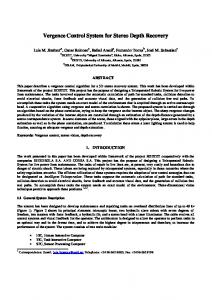
the output node and when CLK goes low, the output regenerates to full swing. This latch consumes a large short-circuit current in the reset mode and zero DC current after full regeneration is achieved. This is illustrated in Fig. 3.7, where the top row shows data and clock input to the latch with a phase offset of 8 ps, and the bottom row shows the two single-ended outputs of the latch.
Figure 3.6: Schematic of type-1 digital latch. This latch is used after the level shifter.
Type-2 static digital latch We can see that the output signal of the type-1 digital latch has a reset phase but the digital XOR gates are designed to operate with full swing digital signal inputs without any reset phase. Thus, we implemented a second type-2 differential digital latch shown in Fig. 3.8 to clean the waveform before sending to the XOR gates. The second digital latch is used to hold the output of the first digital latch during the reset phase. The output is held by a weak latch when clock is high and it follows the input when clock is low. This latch generates a full swing rail-to-rail output signal suitable for XOR gates.
30
Figure 3.7: Top plot shows data and clock with a phase offset of 8 ps. Bottom plot illustrates type-1 latch regeneration to full swing.
Figure 3.8: Schematic of type-2 digital latch. This latch is used after type-1 digital latch.
31
XOR gate The static CMOS XOR gate schematic is shown in Fig. 3.9. Both inputs are full swing and differential. The S1- and S2- are the inverted version of S1+ and S2+, respectively, and they are easily available due to the differential nature of the flip flops. In the event that S1 and S2 are the same, the output is low. When S1 and S2 are different, the pull-down network is active, hence output signal is pulled high by the PMOS transistor.
Figure 3.9: XOR gate used in the phase detector. Four copies are used in the loop to generate UP+, UP-, DN+, and DN- ouput signals. The example shown here generates the signal UP+.
Phase detector transfer characteristics The phase detector input-output characteristics are plotted in Fig. 3.10, which is an indicator of how good an alignment we can get in the closed loop. The plot shows that when the phase difference between data and clock is less than 8 ps, the flip-flop enters the metastable region. But for some part of the metastable region, the flip-flop generates error in the correct direction and hence we will see later that when the loop is closed we achieve better phase alignment between data and clock than 8 ps.
32
Figure 3.10: Phase detector transfer characteristics.
3.3.2
Charge pump
The XOR gates generate full swing pseudo-differential UP/DN signals which go into the charge pump. A pseudo-differential digital charge pump topology shown in Fig. 3.11 is used. The circuit topology of the charge pump is same as the fully differential analog charge pump [18] except that each branch has a separate current source. This is done to prevent shorting of the charge pump outputs through the common source node when the input transistors go into the linear region with large input swing. Recall from Chapter 2 that control line is designed to be high impedance so that charge pump acts as an integrator. The charge pump operates at 1.8 V to get a large control voltage linear range. Since 1.8-V supply is used, the charge pump makes use of 1.5-V transistors and cascoding to prevent transistors from getting stressed. The operation of the circuit is summarized in the Table 3.1. When both UP and DN signals are of the same polarity, then only one of the bottom branches is turned on and hence the current Ibb from the top PMOS current source goes through the bottom NMOS current source, keeping the control voltage constant at its previous value. When UP and DN signals are of different polarity, then both bottom branches are either ON or OFF simultaneously. When both bottom branches are ON, the loop
33
Figure 3.11: Charge pump schematic. The current flow directions are marked for the following inputs. DN+ = UP- = 1.2 V and UP+ = DN- 1.2 V. Ibb current is provided by the loop filter to satisfy current balance at charge pump output node (CP/CN). The parameters values are Ibb = 100 µA and Vref = 0.9 V. Table 3.1: A truth table illustrating charge pump operation UP DN CP 1 1 x 0 0 x 1 0 1 0 1 0
filter sources current Ibb into one of the bottom branches, while when both bottom branches are OFF, the loop filter sinks Ibb current coming from the top PMOS current source. A good charge pump needs constant current source for sourcing/sinking current in/out of the loop filter. The cascoding of the top and bottom branches helps to limit VDS variation of the current sources and hence reduces current variation. The bottom current source VDS is limited to 1.2 − Vt when that particular branch is ON while the top PMOS current source VDS is limited to 1.8−(Vref +Vt). To verify this, we performed a test on the PMOS current source with and without cascoding, the 34
setup of which is shown in Fig. 3.12. We can see from the plot in Fig. 3.13 that current is approximately constant when cascoding is used.
Figure 3.12: PMOS current source load.
Figure 3.13: PMOS current source cascoding benefits.
Common mode feedback Common mode feedback (CMFB) is needed in the charge pump, since any mismatch in the top and bottom current sources can drastically change the voltage level of the 35
output node because of its high impedance nature. The CMFB is implemented by sensing the output voltages CP/CN by unity gain amplifiers. The average value of
Figure 3.14: CMFB DC analysis. the sensed voltage is then compared with the desired output common mode voltage level of 0.9 V and the error signal thus generated is used to control the current of the top PMOS current source. The DC simulation was performed to check the operation of the common mode feedback circuit. Figure 3.14 plots the voltage at the mid-node and at the output of the unity gain amplifiers that are sensing the control voltages CP/CN. As can be seen, mid-node accurately follows the common mode voltage of the charge pump over wide control voltage range. CMFB is a negative feedback circuit and hence we evaluated its phase margin to ensure stable operation. We added 2 pF of capacitance in the feedback path to achieve 90o phase margin; this is plotted in Fig. 3.15. The ac analysis was then done to measure the phase margin of the system.
36
Figure 3.15: CMFB stability test showing 96o phase margin.
Unity gain amplifier The unity gain amplifier used in the CMFB is shown in Fig. 3.16. The unity gain amplifier is designed to have a DC open loop gain of 30 dB and phase margin of 90o.
Output resistance The charge pump acting as an ideal integrator should have large output resistance. Since input transistors act as switches and have low resistance when turned ON, the output resistance of the charge pump is mainly decided by the output resistance of the current sources. The output resistance of a MOSFET in saturation is given by Eq. (3.12) VA Rout= ID
37
(3.12)
Figure 3.16: Schematic of unity gain amplifier. where VA is the early voltage of the device and ID is the drain current through the device. Thus, in order to increase the output resistance we can either increase VA or decrease current ID through the device. The early voltage VA can be increased by increasing the channel length of MOS current sources; in this design we have used channel length of 200 nm for bottom NMOS current sources and channel length of 400 nm for top PMOS current sources. The bottom NMOS current source length is relatively small to avoid excessive capacitance at node X in Fig. 3.11; this is needed to keep the bandwidth of the charge pump high because each time the input transistors turn ON/OFF the node X needs to be charged/discharged. Decreasing current of the current sources is another option to increase output resistance, but decreasing current to a very small value makes the control voltage susceptible to noise from the substrate, charge injection, etc. In our design we used an acceptable current of 100 µA. The output resistance of the device was estimated using DC operating point information. The overall output resistance was calculated to be 7 kΩ.
38
Control voltage linear range One of the design objectives of a good clock data recovery system is to have a large linear range of the control voltage. A large linear range of the control voltage helps to span a large clock frequency range in the LC VCO with a relatively small Kvco. Please note that the large Kvco converts noise on the control line into jitter on the clock output. The linear range of the control voltage was plotted by doing a rail to-rail DC sweep on the control line CP/CN and measuring the currents in the top and bottom current sources. This is shown in Fig. 3.17. We can see that as CP/CN goes below 0.4 V, the bottom current source leaves the saturation region, and when CP/CN goes above 1.4 V, the top current source leaves the saturation region. Thus, we achieved 2-VPP differential control voltage linear range.
Figure 3.17: Single-ended charge pump linear range.
Transient simulation The transient simulation was performed with a pseudo-random bit sequence to check the time domain performance of the charge pump. The phase updates on the charge 39
pump must have sharp edges to increase the phase margin or the stability of the system. The sharp-edged square pulses on the control line mean that any parasitic capacitance on the control line is small. Note that the large loop filter capacitance CP creates an ‘ac’ ground at node Y in Fig. 3.19. The differential charge pump output is shown in Fig. 3.18.
Figure 3.18: Charge pump transient output with PRBS data.
Loop filter The loop filter schematic shown in Fig. 3.19 has an integrating and proportional path to provide phase updates to the PLL loop. The proportional path is implemented with a 100-Ω resistance and the integrating path with a 500-pF capacitance. The integrating capacitance of 500 pF is used for simulation purposes only; in reality, a 10-nF off-chip capacitance will be used. Since the entire loop filter is off-chip, a 1.5-nH inductance is used to model the bond wire inductance. A 400-fF capacitance is added to take into account the pad and routing wire parasitics. This capacitance helps to reduce charge injection on the control line due to switching of input transistors, but this capacitance should not be large because then it makes the system third order [19].
40
Figure 3.19: Loop filter schematic. The loop filter is implemented off-chip. An inductance of 1.5 nH is used to model the bond wire inductance and 400-fF parallel capacitance is added to take into account the pad and routing wire parasitics. Node Y above is the same as node Y in Fig. 3.11 Charge pump summary Supply voltage = 1.8 V Current IC = 100 µA Linear range = 2-VPP differential Output impedance = 7 kΩ CMFB phase margin = 90o Unity gain amplifier: gain = 30 dB, phase margin = 90o
3.3.3
Voltage controlled oscillator
A differentially tuned voltage-controlled oscillator [20] is used to generate the reference clock signal in the CDR. The design of the VCO will be discussed here briefly; for full detail of the design the reader is referred to [21]. A schematic of the VCO is shown in Fig. 3.20. The LC VCO uses a cross-coupled NMOS pair and a tunable LC tank. The binary weighted capacitor banks are used to change the free-running frequency of the VCO. At one particular setting of the capacitor bank, differential frequency tuning is achieved by varactor diodes connected in a bridge fashion. The differential
41
varactor bridge structure allows the use of differential control lines, which improves the common-mode noise rejection of the control lines. The gain of the VCO, kvco, is set to 125 MHz/V. The VCO tail current source uses a current DAC controlled by external bits to adjust the value of the output swing. A capacitor in parallel with the tail current source [22] is used to reduce flicker noise contribution of the tail current source. The VCO achieves phase noise of -110 dBc/Hz at 1-MHz offset. To achieve a differential output swing of 1.15 V, VCO burns 6.5 mW of power.
42
Figure 3.20: Schematic of a 6.25-GHz VCO presented by Bhatia [21]. A large tuning range is achieved through the use of a binary weighted capacitor bank and differen tially biased PN junction varactors. A capacitor in parallel with the tail current DAC is used to reduce the phase noise contributions from the current source.
43
3.3.4
Clock buffer
The clock buffer shown in Fig. 3.21 is one of the most power hungry blocks in the whole CDR system. The purpose of the clock buffer is to convert a sinusoidal clock into a full swing digital clock with small rise and fall times. The sinusoidal VCO clock is ac coupled into the first gain stage of the clock buffer, which is designed to have a gain of 2. The later buffers are implemented in tapered fashion, slowly increasing the drive strength to a level where it can drive the large clock load of the phase detector. The input and output waveform of the clock buffer are plotted in Fig. 3.22. We can see that we get nice sharp-edged clock coming out of the clock buffer; this simulation includes all the load of phase detector that the clock needs to drive.
Figure 3.21: Clock buffer schematic.
Figure 3.22: Clock buffer input and output waveforms. The input to the clock buffer is a 1.1-VPP differential output of the VCO and the output is a sharp-edged 2.4-VPP differential digital signal.
44
3.4 3.4.1
Closed Loop Performance Testing with pseudo random bit sequence
After designing each component of the clock recovery unit, the transient simulation was performed on the postlayout extracted netlist to analyze the closed loop locking behavior of the CDR. The input data stream is an NRZ pseudo-random bit sequence. In an actual chip, frequency acquisition will be performed through external tuning of the control voltage, so for simulation purposes we initialize the control voltage to a value which brings clock frequency close to the data frequency. Figure 3.23 shows the control voltage plot and we see that the loop has a settling time of approximately 200 ns. Once the loop is locked, it is important to check the alignment of clock and data as shown in Fig. 3.24. The plot shows that the clock falling edge lies in the center of the data-eye and hence can be used to slice the data with maximum timing and noise margins. The sliced data-eye diagram is shown in Fig. 3.25, which shows a wide-open eye.
Figure 3.23: Control voltage plot of the CDR is closed loop. The plot shows shows that the control voltage is settled after 200 ns.
45
Figure 3.24: Clock and input data-eye diagram. The eye diagram shows that the clock falling edge lies in the center of the data-eye and hence can be used to sample the data with maximum timing and noise margins.
Figure 3.25: Eye diagram of the sliced data, showing a wide-open eye.
46
3.4.2
Jitter tolerance
The jitter tolerance tests were performed to verify the CDR’s ability to track input data jitter. Two jitter tolerance tests were performed, with the first test applying a sinusoidal phase jitter of 0.15 UI at 4 MHz on the data and the second test having a sinusoidal phase jitter of 1.5 UI at 400 kHz applied to the data. The circuit simulation results are discussed next.
0.15-UI sinusoidal jitter at 4 MHz The jitter test is performed with continuous switching data so that error can be detected easily. A stream of continuous switching data with no jitter is applied to the CDR from 0 ns to 250 ns in order to lock the loop to the data source. After 250ns has elapsed, a 0.15-UI sinusoidal phase jitter at 4 MHz is applied to the data. The control voltage plot in Fig. 3.26 shows that control voltage modulates as the loop clock tracks the jitter. The plot in Fig. 3.27 shows the integrated voltage across the loop capacitor; we can see that control voltage is modulated at jitter frequency to track the data jitter. The plot in Fig. 3.28 shows the eye-diagram of the sliced data. The data bits are sliced correctly since the eye-diagram shows no continuous 1 or 0 for this continuously switching input data stream. Also, we see more zero crossing spread because the clock phase keeps changing in order to track the input data jitter.
1.5-UI sinusoidal jitter at 400 kHz Figure 3.29 shows the control voltage plot for the jitter tolerance test of 1.5 UI at 400 kHz. Jitter is introduced after 250 ns has elapsed. We see from Fig. 3.30 that the control voltage is modulated slowly here as compared to the previous plot because of lower jitter frequency.
47
Figure 3.26: Control voltage plot for a sinusoidal input jitter of 0.15 UI at 4 MHz. The control voltage is modulated at jitter frequency.
Figure 3.27: Filtered control voltage plot more clearly showing 4-MHz modulations on the control line.
48
Figure 3.28: Eye diagram of the sliced data for 0.15-UI jitter at 4 MHz. The data bits are sliced correctly since the eye diagram shows no continuous 1 or 0 for this continuously switching input data stream.
Figure 3.29: Control voltage plot for sinusoidal input jitter of 1.5 UI at 400 kHz. The control voltage is modulated at jitter frequency.
49
Figure 3.30: Filtered control voltage plot more clearly showing slow 400-kHz modu lations on the control line. The plot in Fig. 3.31 shows the eye-diagram of the sliced data; it can be seen that there are no consecutive ones or zeros for continuous switching data and hence the data is detected correctly.
Figure 3.31: Eye diagram of the sliced data for 1.5-UI jitter at 400 kHz. The data bits are sliced correctly since the eye diagram shows no continuous 1 or 0 for this continuously switching input data stream
50
3.4.3
Consecutive identical digit (CID) test
The CID test is used to verify whether the loop is locked or not, for a long sequence of 1’s or 0’s. To perform this test, the CDR is allowed to lock onto the incoming data stream and, under locked condition, 500 identical data bits are sent in to the system. Note that the phase updates are available to the loop only when data transition occurs and thus if there are no data switching for a long time the control voltage can drift. The amount of CIDs the loop can tolerate depends on the output resistance of charge pump; a large output resistance prevents the drift in the control voltage. As can be seen from the control voltage plot in Fig. 3.32, the system is locked after 500 identical digits because control voltage does not show any large drift. But it is not clear whether the loop lost lock for a few bits after the data started switching. To investigate this, the plot (B) of Fig. 3.32 zooms in on the control voltage in the region marked with the dashed square box. We see that the control voltage is constant for some time when the data switching began again, indicating that the loop has developed some phase error and is trying to make corrections. The plot (C) of Fig. 3.32 shows data and clock alignment just before and after data switching starts. We see that the phase error is small and clock and data are still aligned with data transition happening near the clock rising edge.
51
Figure 3.32: CID test results. Plot (A) is the control voltage plot, the area in the dashed box highlights the time when data switching begins again, after 500 identical bits. Plot (B) zooms in on the control voltage in the area marked with the dashed box. Plot (C) shows data and clock alignment just before and after data switching starts.
52
Table 3.2: CDR power summary Block Power Consumption LC VCO 5 mW Clock Buffer 16 mW (digital Phase detector section) 5.1 mW Phase detector (analog section) 5.4 mW Charge pump 1.8 mW Miscellaneous 2.7 mW Total 36 mW
3.4.4
Power consumption
The postlayout power consumption summary of each block of the 6.25-Gb/s clock data recovery system is listed in Table 3.2. We can see from the table that clock buffer consumes the largest power while other blocks are not that power hungry. This is not surprising because for best operation of digital latches we need sharp-edged clocks, which consume power. The postlayout total power consumption of the implemented CDR amounts to 36 mW from a 1.2-V power supply, where the clock buffer consumes 16 mW of power and the core CDR circuit 20 mW. This results in a total consumption per data rate for the core CDR of 3.2 mW/(Gb/s). Typically, core CDR circuits in 90-nm CMOS technology consume 3.9 mW/(Gb/s) [23].
53
CHAPTER 4 RECEIVER BANDWIDTH EXTENSION USING NEGATIVE CAPACITANCE CIRCUITS 4.1
Motivation
The motivation for this work is to increase bandwidth and improve impedance match ing, or s11, of high-speed receiver circuits operating in the gigahertz range. Gonzalez [24] discussed the problem of broadband impedance matching for high-speed RF cir cuits. The input impedance of a typical receiver can be represented as a termination resistor in parallel with the parasitic capacitance at the input of the receiver. The parasitic capacitance at the input is mainly due to the ESD device capacitance and the pad capacitance. The impedance matching and bandwidth at the receiver can be improved by reducing the net parasitic capacitance at the input node. The pad capacitance, although large, cannot be reduced significantly because of the metal stack and minimum pad opening constraints imposed by the foundry. The ESD de vice capacitance can be reduced by reducing the device size, but that degrades the attainable ESD protection level. ESD protection level is directly proportional to ESD device size at the pad, which in turn is proportional to the device capacitance. Hence, large ESD protection levels generally demand large device capacitance, which severely degrades receiver bandwidth. Thus, we need techniques to enhance receiver bandwidth without degrading the ESD performance. Negative capacitance circuits have been used extensively in the recent past to cancel node capacitances. Comer et al. [25] demonstrated the use of negative capaci tance circuits to extend the bandwidth of high-gain CMOS stages. Galal and Razavi 54
[26] used negative capacitance circuits in addition to T-coil for receiver bandwidth extension. Yoo et al. [27] used negative impedance circuits to increase the gain bandwidth product of a limiting amplifier. In this thesis, we will explore in detail negative capacitance circuits for receiver bandwidth extension. We will also present a novel Gm-boosted negative capacitance circuit for further bandwidth extension. This chapter begins by modeling receiver input impedance; we then explore NMOS cross-coupled and Gm-boosted negative capacitance circuits. Finally, we demonstrate their application to extend receiver bandwidth and evaluate ESD performance of the overall receiver.
4.2
Receiver Input Impedance Model
The conventional IC receiver termination consists of a 50-Ω matching resistance and some parasitic capacitance due to on-chip pad, ESD protection circuit, and receiver input transistors. For first-order analysis, receiver input impedance due to parasitic capacitance and termination resistance can be modeled as shown in Fig. 4.1. The expression for the admittance is shown in Eq. (4.1).
Figure 4.1: Simplified receiver input model. Typically in a receiver r = 50 Ω and c = 300 fF.
YIN = 1r +jωc
55
(4.1)
It can be seen that the imaginary component of input admittance YIN is a function of the frequency of operation. The receiver input bandwidth (f−3bB) and impedance matching (S11) depend on the value of YIN. Ideally we want YIN to be purely resistive, hence having zero imaginary part, which can be done by making capacitance ‘c’ zero. The capacitance ‘c’ can be reduced by placing a circuit which has a negative capacitance in parallel with YIN, as shown in Fig. 4.2.
Figure 4.2: Model of an improved receiver input, using a parallel negative capacitance to reduce the net input pad capacitance.
YIN = 1r + jωc − jωcneg
(4.2)
The expression for the modified admittance is shown in Eq. (4.2). The net input capacitance is reduced by the amount of negative capacitance ‘cneg’. If the added negative capacitance is equal to the positive capacitance, then the system will have infinite input bandwidth (f−3dB) and impedance matching (S11). While there are no true negative capacitors, one can design a circuit whose admittance has a negative imaginary component in a limited frequency range. If the circuit is carefully designed it will look like a negative capacitance in the frequency band where capacitance reduction is needed.
56
4.3
NMOS Cross-Coupled Negative Capacitance Circuit
As the name suggests, the purpose of a negative capacitance circuit is to provide a reactance which is negative of the positive capacitance circuit. Since two capacitances in parallel at a circuit node are added together, a negative capacitance in parallel with a positive capacitance can help to reduce the overall positive capacitance at a circuit node. Reduction in overall positive capacitance at a node helps to increase circuit bandwidth as shown by Eq. (4.3), where c is the net positive capacitance.
f−3dB =
1 2πrc
(4.3)
An NMOS cross-coupled pair with capacitive degeneration, shown in Fig. 4.3, can be used to generate a negative capacitance between two nodes of a differential circuit. Because this is a differential circuit, for small-signal analysis, nodes nodeP and nodeN are equal in magnitude and opposite in phase. The two branches in Fig. 4.3 are symmetrically biased by two equal MOS current sources, M3 and M4, and contain two transistors M1 and M2 which have equal Gm values. The capacitance CP is added to account for device and interconnect parasitic capacitance at the drain of transistors M3 and M4. The capacitance CC is added for capacitive degeneration of two branches, and it will be shown later that the negative capacitance obtained from this circuit is proportional to the value of CC. To analyze the negative capacitance circuit we will use differential impedance, which by definition is the impedance that the differential signal sees looking into the circuit. The differential impedance is measured as VAC/i where VAC and i are defined in Fig. 4.3. The small-signal analysis shows that differential impedance between nodes nodeP and nodeN is given by Eq. (4.4), where gm is the transconductance of transistors M1 and M2, and ro is output resistance of current sources M3 and M4.
57
To keep the equation simple and easy to understand, it does not consider gate-source capacitance of transistors M1 and M2 . It can be seen that if we ignore ro and CP, the circuit gives negative capacitance whose value is directly proportional to the value of capacitance CC.
Zneg = −
2 + gm
1
1
− 1/s(−CC )
1 (2ro ) (1/sCP )
≈−
2 + 1 gm s(−CC)
(4.4)
Figure 4.3: Negative capacitance circuit. To better understand the negative capacitance circuit, we can rewrite Eq. (4.4), where the second term is represented as Zφ.
2 Zneg = − gm − Zφ where
Zφ 1
=
1/sCC 1
+
(4.5)
1 (2ro)(1/sCP)
As shown in Fig. 4.4, Zφ is the impedance seen looking down from the source of transistors M1 and M2; also shown is a simple connection of negative impedances in cascade which can be used to model the entire negative capacitance circuit. The model shows that the NMOS cross-coupled pair helps to invert the sign of impedance 58
Zφ connected between its source terminals. This is an important observation since one can choose Zφ at will and use an NMOS cross-coupled pair to invert the sign of Zφ.
Figure 4.4: Simplified drawing of negative capacitance circuit. Figure 4.5 shows a plot of the real and imaginary components of the input impedance of receiver in Fig. 4.1. This plot is generated by connecting an ac current source at the input terminal and simulating voltage at the same node. We can see from the plot of reactance that it has a negative inductance region where impedance increases in negative direction as frequency increases, followed by a capacitive region where the magnitude of the impedance decreases with frequency. The expression for input impedance is shown in Eq. (4.6).
ZIN = 1 r
1 r ωcr2 1+(rωc)2 ·j +ωc = 1+(rωc)2 −
(4.6)
Figure 4.6 plots the real and imaginary components of impedance Zneg, as given by Eq. (4.4). We can see that this reactance is negative of the reactance plot shown in Fig. 4.5; it has a positive inductance region and a negative capacitance region. The amount of negative capacitance obtained can be increased or decreased, depending on the value of CC. 59
Figure 4.5: Simulated real and imaginary component of ZIN in Fig. 4.1. Typically in a receiver r = 50 Ω and c = 300 fF.
Figure 4.6: Simulated real and imaginary components of Zneg. The plot is obtained by dissipating 4 mA of total current in the NMOS cross-coupled negative capacitance circuit and using a degeneration capacitance of 400 fF.
60
For best cancellation effects, the positive capacitance region of Fig. 4.5 and the negative capacitance region of Fig 4.6 should lie in the same frequency band. These capacitance regions occur for frequencies greater than the one at which the reactance peaks. The magnitude of the peak reactance and the frequency at which it happens can be derived by differentiating the imaginary component of Eq. (4.4) and equating it to zero, likewise for Eq. (4.6). For the negative capacitance circuit, the value of peak reactance and the corresponding frequency are given by Eqs. (4.7) and (4.8). For the receiver, the peak reactance and corresponding frequency are given by Eqs. (4.9) and (4.10). If the two capacitance regions are not aligned, we must analyze how to move the negative capacitance region to either low or high frequency. Since the negative capacitance region comes after the peak reactance point, it can be moved by changing the frequency of the peak reactance. Equation (4.8) reveals that in order to shift the negative capacitance region to higher frequency band, degeneration capacitance CC or output resistance ro must be decreased. But decreasing CC reduces the amount of negative capacitance, as shown in Eq. (4.4), and thus limits the amount of cancellation possible. So we must decrease output resistance ro of transistors M3 and M4, which can be done by increasing current in these transistors.
Maximum Reactance = −ro
1 ωpeak = (2ro(CC +
(4.8) CP2)
Peak Reactance = −r2
ωpeak =
61
1 rc
(4.7)
(4.9)
(4.10)
The real part of the negative capacitance circuit in Fig. 4.6 shows a large value at low freq (DC). This also agrees with Eq. (4.11) obtained by putting s=0 in Eq. (4.4), which shows high impedance due to large output resistance of MOS devices. Although large negative resistance can cause oscillations in circuits [28] it will be shown later in Section 4.6 that in this application, a large negative real part is beneficial.
Zneg(s = 0) = −
2 2 − gm ro
(4.11)
The frequency response of the real part shows that this large negative resistance starts to decrease at higher frequency due to shunting of ro by capacitances CC and CP. The cutoff frequency of the real component of Zneg is same as that given in Eq. (4.8). The cutoff frequency marks the beginning of the region where real part drops and starts to affect the input impedance matching of the receiver. To avoid complexity, until now analysis has been done without taking into consid eration Cgs of transistors M1 and M2. A simple analysis is done to check the depen dence of Zneg on Cgs of transistors M1 and M2, while neglecting output resistance of MOS devices and parasitic capacitance CP. This analysis brings out accurately the bandwidth limitation of the negative capacitance circuit at high frequency. Figure 4.7 shows the small-signal model used for recomputation of Zneg.
Figure 4.7: Small signal model of negative capacitance circuit.
62
The small signal analysis yields Eq. (4.12), which shows that the pole appears at ωT which is also defined in Eq. (4.12). It can be seen that the bandwidth limitation of the negative capacitance circuit originates from ωT , which can be increased by either increasing transconductance (gm) or reducing Cgs of transistors M1 and M2. Since increasing device size of transistors M1 and M2 increases both gm and Cgs, benefits start to decrease when device size becomes large. The better way to overcome this tradeoff is to increase the current through MOS devices, which increases gm without affecting Cgs. It is important to understand the techniques of increasing the -3 dB bandwidth of the negative capacitance circuit, because the circuit will be used to increase the -3-dB bandwidth of some other circuit and it must have -3-dB bandwidth larger than the circuit whose bandwidth is to be extended. Cgs CC +2
Zneg =
− gm 1+sωT
sCC −1
where ωT =
4.4
(4.12)
gm Cgs
Gm-Boosted Negative Capacitance Circuit
The Gm-boosted negative capacitance circuit shown in Fig. 4.8 is similar to the cross coupled negative capacitance circuit, except that a gain stage A is introduced in the cross-coupled path. The introduction of gain stage A increases the effective Gm of transistors M1 and M2 by an amount A.
63
Figure 4.8: Gm-boosted negative capacitance circuit. The gain stage A is introduced in the cross-coupled path. The small-signal analysis shows that differential impedance is given by Eq. (4.13); as for Eq. (4.4), this equation does not consider Cgs of transistors M1 and M2 for simplicity.
2 1 2 1 Zneg=−Agm + As(−CC)−A2ro(1/sCP) ≈− Agm + As(−CC)
(4.13)
Assuming that gain stage A has infinite bandwidth, we see from Eq. (4.13) that negative capacitance is multiplied by gain A, while the real part is reduced by gain A. The increase in negative capacitance leads to better cancelation of positive capac itance while the effect of smaller negative real part may be good or bad, depending on the application. A simple analysis can be done to show that reactance of Zneg decreases with increasing gain magnitude A as predicted by Eq. (4.13). This is shown in Fig. 4.9 where ideal gain elements are used for three gain settings of A equal to 1, 2, and 3. Note that reactance decreases and negative capacitance increases as gain increases, and also that the frequency of peak reactance remains the same and is independent of the gain. 64
Figure 4.9: Reactance plot of Zneg for three gain settings (A=1,2,3). The plot is obtained from circuit simulation of Gm-boosted negative capacitance circuit using a degeneration capacitance of 45 fF. The real component of Zneg behaves similarly and its resistance decreases as the magnitude of gain A increases, as predicted by Eq. (4.13). Figure 4.10 plots the variation of the real part of Zneg for three gain settings of 1, 2, and 3. Note that gain A = 1 corresponds to the case of the NMOS cross-coupled negative capacitance circuit. We can see that as gain increases, the real part of Zneg decreases. Although the Gm-boosted negative capacitance circuit increases negative capaci tance by amount A, one can argue that the same effect can be obtained by increasing the value of capacitance CC in the NMOS cross-coupled negative capacitance circuit. But as argued in Section 4.3, increasing CC pushes the frequency of reactance peak, or negative capacitance region, towards low frequency, degrading cancelation. In contrast, the Gm-boosted negative capacitance circuit increases negative capacitance but keeps the frequency of reactance peak or negative capacitance region at the same place. To verify the preceding arguments about the superiority of the Gm-boosted neg 65
Figure 4.10: Real part of Zneg for three ideal gain settings (A=1,2,3). The plot is obtained from circuit simulation of Gm-boosted negative capacitance circuit using a degeneration capacitance of 45 fF. ative capacitance circuit, the reactance of both the NMOS cross-coupled and the Gm-boosted negative capacitance circuit were simulated and plotted together in Fig. 4.11. Notably in this example, a real gain element is used rather than an ideal one with infinite bandwidth. Here, we have used a simple resistive-loaded differential amplifier, as shown in Fig. 4.12, as the gain element because it can provide good bandwidth for a moderate gain of 2 to 5. A resistor RC is added in series with the supply terminal for the adjustment of output common mode level to the desired level. In Fig. 4.11, ωpeak is observed to be the same for the two circuits which use the same capacitance CC, while the reactance magnitude decreases by a factor A for the Gm-boosted case. This confirms that the Gm-boosted negative capacitance circuit can provide a large negative capacitance at high frequencies. A small-signal model taking Cgs of transistors M1 and M2 into consideration, and ignoring output resistance of MOS devices and parasitic capacitance CP, is shown in Fig. 4.13.
66
Figure 4.11: Reactance comparison of NMOS cross-coupled and Gm-boosted negative capacitance circuit.
Figure 4.12: Gain stage used in Gm-boosted negative capacitance circuit.
67
Figure 4.13: Small signal model taking Cgs into consideration. Equation (4.14) is an expression for the differential impedance between nodes nodeP and nodeN of the Gm-boosted negative capacitance circuit. It can be seen that one of the major benefits of Gm boosting is that the bandwidth of the negative capacitance circuit (ωT) is increased by the amount of gain A (AωT). Equation (4.14) does not consider bandwidth limitation of gain stage A; it is important that the gain stage have bandwidth larger than ωT ; otherwise, the benefit of Gm-boosting will not be significant. Cgs +2 CC
AsCC −11 + − sAgm
Zneg =
(4.14) AωT
where ωT =
gm Cgs
Any amplifier stage with bandwidth of the order of ωT can be used to get the benefits of Gm boosting. It will be shown later in Section 4.5 that for our application of receiver bandwidth extension we do not need a separate gain stage; instead, one of the gain stages of the receiver can be used for this purpose.
68
4.5
Receiver Bandwidth Extension
A typical receiver of a gigabit per second link shown in Fig. 4.14, consists of a cascade of linear gain stages to amplify incoming small signals to signal swings which can be easily detected by internal core circuits. A large 100-nF off-chip ac coupling capacitor is usually used to decouple the dc level of the receiver from that of the channel. This is followed by a board or pin capacitance of 300 fF, and a 2-nH bond wire inductance. ESD device and bond pad capacitance are usually of the order of 300 fF and 200 fF, respectively. In order to properly terminate the transmission line we use a 50-Ω on-chip termination resistor. Depending on the application, different numbers of gain stages are used to get the desired gain.
Since receiver input has relatively
Figure 4.14: Differential receiver. The schematic shows package parasitics and receiver gain stages. large capacitance, NMOS cross-coupled or a Gm-boosted negative capacitance can be used in the receiver front-end to cancel some part of the receiver input capacitance. Figure 4.15 shows a receiver with an NMOS cross-coupled negative capacitance circuit added at the input pad. Two 46-Ω termination resistor biases the negative capacitance circuit through a 1.2-V reference supply voltage. A simple biasing circuit shown in
69
Figure 4.15: Receiver with NMOS cross-coupled negative capacitance circuit. Fig. 4.16 is used, where current from an external current source flows into a diode connected NMOS transistor and is then mirrored in different analog blocks, including the negative capacitance circuit.
Figure 4.16: Biasing circuit. The current source uses channel length of 200 nm and an external current source of 250 µA. A 2.1-mA current flows through each of the bias transistors M3 and M4 in the negative capacitance circuit. This relatively large current is needed in the negative capacitance circuit to push the ‘negative capacitance’ region of the circuit to high frequency. For design purposes, admittance analysis will be used, because two parallel admittances can be simply added to obtain the overall admittance. Thus, instead of maximizing total reactance we will minimize susceptance. The susceptance of the 70
standalone receiver with bond wire inductance shorted out, and the susceptance of the receiver with NMOS cross-coupled negative capacitance circuit are plotted in Fig. 4.17. The bond wire inductance is shorted out so that we can keep the analysis simple. The expression for the admittance of the standalone receiver with bond wire shorted out is shown in Eq. (4.15) and we can see that its susceptance increases with frequency as plotted in Fig. 4.17.
YIN =
1 + sc r
(4.15)
Figure 4.17: Susceptance plot of the standalone receiver and NMOS cross-coupled negative capacitance circuit.
The susceptance of the negative capacitance circuit is the imaginary part of the inverse of Eq. (4.4). Since the susceptance equation becomes quite complex we will analyze its behavior graphically. At low frequency, dc reactance is zero and thus susceptance is also zero; as frequency increases further, the negative capacitance effect kicks in, and we see negative values of susceptance in the plot of Fig. 4.17. As 71
frequency increases beyond the susceptance peak, higher-order poles dominate and we start to lose the negative susceptance effect; instead, it starts to behave like a positive susceptance similar to that of receiver in Eq. (4.15). The two admittances YIN and Yneg are connected in parallel at the receiver input and hence can be added together to get the resultant admittance of the combined cir cuit. The plot in Fig. 4.18 shows final susceptance along with the susceptance of the standalone receiver and NMOS cross-coupled negative capacitance circuit. The plot shows that the susceptance of the negative capacitance circuit helps to first reduce the susceptance of the combined circuit and then to increase it later, when the sus ceptance of the negative capacitance circuit becomes positive. Both of these features are desirable, since reduction of net susceptance near the corner frequency helps to increase the bandwidth of the circuit, while increased positive susceptance later helps to attain sharp rolloff in the gain plot. In high-speed links, sharp rolloff of receiver gain after -3-dB frequency is desirable, to limit the channel noise amplification. Note that we can increase the negative susceptance further by increasing capacitance CC of the negative capacitance circuit, but the circuit simulated in Fig. 4.18 was optimized to give a maximally flat gain response with little peaking, shown in Fig. 4.19. The gain of the circuit in Fig. 4.15 is simulated by connecting differential ac sources at terminals IN+ and IN- and measuring output at Pad+/Pad-. The gain response of the receiver with and without NMOS cross-coupled negative capacitance circuit is shown in Fig. 4.19. Note that the circuit simulation of both cases includes bond wire inductance. The plot shows that the receiver without the negative capac itance circuit has a -3-dB frequency of 5.2 GHz, while the receiver with the NMOS cross-coupled negative capacitance circuit has a -3-dB frequency of 7.7 GHz, a band width extension of 2.5 GHz or 50%. Figure 4.19 shows that the NMOS cross-coupled negative capacitance circuit gives input bandwidth improvement over the standalone receiver circuit. Now we will show that we can further extend the bandwidth at no
72
Figure 4.18: Susceptance plot showing cancelation effect. The NMOS cross-coupled negative capacitance circuit uses 2-mA current in each branch and a degeneration capacitance of 400 fF.
Figure 4.19: Bandwidth comparison of standalone receiver and receiver with NMOS cross-coupled negative capacitance circuit. The bond wire inductance is included in both the configurations. The simulation results shows that the receiver with the NMOS cross-coupled negative capacitance circuit shows a input bandwidth improve ment of 50% over the receiver without any negative capacitance circuit.
73
extra power cost using the Gm-boosted negative capacitance circuit, shown in Fig. 4.20. The circuit is similar to the NMOS cross-coupled negative capacitance circuit, except that a Gm-boosted negative capacitance circuit is added at the receiver in put using the first stage of the receiver amplifier as the gain stage for Gm boosting. Discussion in Section 4.4 showed that large bandwidth gain stage A is required for the best bandwidth extension results; for this purpose, Miller capacitance CM is used after the first receiver amplifier to extend its bandwidth. The positive Miller effect demonstrated in Fig. 4.21 presents negative capacitance at the output of the first receiver amplifier, which helps to increase its bandwidth.
Figure 4.20: Receiver with Gm-boosted negative capacitance negative circuit.
Figure 4.21: Positive Miller effect.
74
The susceptance comparison and cancelation effect are shown in Fig. 4.22. Note that the Gm-boosted negative capacitance circuit gives a negative value of susceptance up to higher frequency, and hence is able to extend receiver bandwidth. Also note that the susceptance of the Gm-boosted negative capacitance circuit increases sharply once it becomes positive, which helps in limiting noise amplification.
Figure 4.22: Susceptance comparison and cancelation effect. Figure 4.23 shows the single-ended gain response, generated similarly to that shown in Fig. 4.19, comparing performance of the standalone receiver, receiver with NMOS cross-coupled negative capacitance circuit, and receiver with Gm-boosted neg ative capacitance circuit. The -3-dB frequency of the receiver with Gm-boosted nega tive capacitance circuit is 8.9 GHz, an extension of 15% over the NMOS cross-coupled circuit. Note that this bandwidth extension is achieved without additional power con sumption. It is useful to have an idea about the maximum bandwidth extension that can be achieved with the Gm-boosted negative capacitance circuit because its performance is highly dependent on the bandwidth of gain stage A. Figure 4.24 shows all the
75
previous gain plots along with the gain response using an ideal amplifier with infinite bandwidth and the same gain as that of the first stage of the receive amplifier. The -3-dB frequency of the receiver with ideal gain Gm-boosted negative capacitance circuit is 10.28 GHz, an extension of 35% over the NMOS cross-coupled circuit. Note that more bandwidth extension can be achieved by increasing gain while keeping bandwidth high, but this is difficult to achieve due to the gain-bandwidth tradeoff inherent in amplifiers.
Figure 4.23: Bandwidth extension comparison of three cases: the standalone receiver, receiver with NMOS cross-coupled negative capacitance circuit, and receiver with Gm-boosted negative capacitance circuit. The receiver with Gm-boosted negative capacitance circuit shows 15% bandwidth improvement over the receiver with NMOS cross-coupled negative capacitance circuit.
76
Figure 4.24: Bandwidth extension comparison of three cases, including the ideal gain stage with a gain of 2.4.
4.6
Receiver Input Impedance Matching
Impedance matching is important in high-speed links for maximum power transfer from transmitter to receiver. For matching purposes an “absolute” 100-Ω differential impedance is required to suppress reflections at the receiver end of the transmission line, although at high frequencies, parasitics at the receiver input tend to reduce overall input impedance, causing reflections and corruption of incoming signals. In this section we will analyze the receiver with NMOS cross-coupled and Gm-boosted negative capacitance circuits from an impedance matching point of view. As discussed in Section 4.2, reduction in net positive capacitance at receiver input makes ZIN predominantly resistive, which helps to improve input impedance matching at the receiver. At low frequencies, differential input impedance of the receiver in Figs. 4.15 and 4.20 is a parallel combination of termination resistor and negative capacitance circuit, since bond wire inductance and parasitic capacitance are short and open, respectively.
77
Impedance of negative capacitance circuits is purely resistive at low frequencies and its value depends on circuit parameters like Gm , ro, and gain A. A large negative real part of Zneg is desirable because, in the case of parallel combination of two resistors, smaller resistance dominates. Both Gm-boosted and NMOS cross-coupled negative capacitance circuits have relatively large negative real part as compared to 50-Ω termination which is good for matching. The comparison of the real parts of the NMOS cross-coupled and Gm-boosted negative capacitance circuits in Fig. 4.10 showed that the real part of the latter is reduced by the factor of gain A. This is not a big problem since termination resistance can be adjusted to get 50-Ω input impedance, and that is why a termination resistor of 39 Ω is used for the receiver with Gm-boosted negative cap circuit while 46 Ω is used for the NMOS cross-coupled one. Either impedance analysis or S-parameter analysis can be done to evaluate match ing performance of a receiver using a negative capacitance circuit. But typically, matching specifications are defined in terms of S11. The value of S11 below -10 dB is considered a good figure and it is defined as the input reflection coefficient with outputs properly terminated. To measure S11 of our receiver in Figs. 4.14, 4.15, and 4.20, we connected a port with 100-Ω impedance between terminals IN+ and IN- and performed S-parameter analysis. Figure 4.25 compares S11 of the standalone receiver and the receivers with NMOS cross-coupled and Gm-boosted negative capac itance circuits. We see 25% improvement in frequency, at which S11 is -10 dB for the receiver with the NMOS cross-coupled negative capacitance circuit. An additional improvement of 15% can be achieved if we implement the Gm-boosted negative ca pacitance circuit. It is worthwhile to point out that the results are consistent with the amount of bandwidth extension obtained for three cases in Section 4.5.
78
Figure 4.25: S11 comparison of standalone receiver and receivers with NMOS cross coupled and Gm-boosted negative capacitance circuits. The receiver with NMOS cross-coupled negative capacitance circuit shows 25% improvement in frequency, when S11 is -10 dB, over the receiver without any negative capacitance circuit. The receiver with Gm-boosted negative capacitance shows a 15% improvement in frequency, when S11 is -10 dB, over the receiver with NMOS cross-coupled negative capacitance circuit.
4.7
ESD Performance
The dual diode based ESD protection is used at the receiver input for its fast turn on, small parasitic capacitance, and good ESD protection capability [26]. The diodes pcell available in the IBM design kit are used as ESD structures. Figure 4.26 shows the input receiver with the dual diode based ESD protection. The ESDVPNP diode is used as a top diode to discharge the pad to the VDD bus for positive zaps while the ESDNDSX diode is used as a bottom diode to discharge the pad to the VSS bus for negative zaps. The ESDVPNP diode is created by a P+ contact in the NWELL region, while ESDNDSX is created by two adjacent stripes of P+ and N+ doped regions, where the P+ region is formed by the substrate. The plot in Fig. 4.27 shows simulated I-V characteristics of two diodes. The turn-on voltage is 1 V for both, while on-resistance is 0.2 Ω for the ESDVPNP, and 0.15 Ω for the ESDNDSX diode. The small on-resistance of the diodes is desirable, 79
Figure 4.26: Dual-diode based ESD protection. because large current flow during an ESD event will produce only a small voltage drop across the diode.
4.7.1
HBM discharge test
The HBM ESD discharge model presented by Mergens [29] is used to simulate an ESD event. Figure 4.28 shows the discharge model, with the values labeled for an HBM event. To simulate a 2-kV HBM event, a 94.8-pF capacitor initially charged to 2 kV is discharged through a 1.5-kΩ resistor to the device under test.
80
Figure 4.27: Diode I-V characteristics.
Figure 4.28: HBM discharge model.
81
For our case, an HBM discharge event between two IO pads is the worst case because that leads to the maximum voltage buildup at the pad during an ESD event. Figure 4.29 shows the simulation setup for the HBM discharge. The ESD zap is applied to one pad while some other pad is grounded. An RC-triggered power clamp available in the IBM design kit is used to discharge the VDD supply bus to the VSS ground bus during ESD. The supply bus resistance is important in ESD system design because large current flow during ESD can lead to large voltage drop across the bus resistance, consequently raising the clamped voltage at the pad. For simulation purposes 1-Ω bus resistance is used to account for supply bus resistance.
Figure 4.29: Two-pin HBM stress setup. A decoupling capacitance of 200 pF is connected between the VDD supply bus and the VSS supply bus. The positive ESD zap is applied at one pad and ground to another pad while all other pads are floating. Figure 4.30 shows voltage at the pad during an HBM stress event. The voltage at the pad initially rises and turns on the ESD diode and power clamp, discharging the zapped pad. Some ringing is observed in the pad voltage due to the presence of bondwire inductance. 82
Figure 4.30: Simulated voltage at pad during 2-kV HBM stress. Figure 4.31 shows supply and ground potential during 2-kV HBM stress. It can be seen that the internal supply voltage with respect to ground does not exceed 2.2 V. The normal supply voltage of the receiver is 1.8 V, and simple resistive-loaded differential amplifiers, as shown in Fig. 4.12, are used as amplifier stages. During ESD, the bias node in Fig. 4.16 is at potential close to VSS. It is shown in [30] that, for 90-nm CMOS process, gate-oxide breakdown voltage is around 8.6 V for input buffers that use cascoding and where the gate-source potential of the bottom transistor is equal to VT. The ESD device size used in our design will safely give an ESD protection level of 3 kV because the pad voltage remains well below the oxide breakdown limit of 8.6 V, as shown in Fig. 4.32 Since transistors used in the negative capacitance circuit are connected at the pad (Figs. 4.15 and 4.20), we must also analyze their ESD performance for the setup shown in Fig. 4.29. The current sources of both the negative capacitance circuits have a gate-source potential of close to zero and hence they are off. The gate of transistor M1, in Fig. 4.15, is coupled to Pad+ in case of the NMOS cross-coupled negative capacitance circuit. While the same transistor gate in case of Gm-boosted
83
Figure 4.31: Simulated supply voltages during 2-kV HBM stress. negative capacitance circuit, in Fig. 4.20, is connected to VDD through the load resistance of gain stage A. The VDD supply voltage during ESD event is same for both the negative capacitance circuit and is shown in Fig. 4.31. Since bottom current sources are off, the source of transistor M1 is at potential V(Pad+)-VT for the NMOS cross-coupled negative capacitance circuit and at potential VDD-VT for the Gm-boosted negative capacitance circuit. This means that the VDS of transistor M1 would be smaller for the NMOS cross-coupled negative capacitance circuit than the Gm-boosted negative capacitance circuit. Note that during an ESD event, smaller VDS of transistor is preferred to prevent it from going into snap-back mode. Both circuits perform well for a 3-kV HBM stress, as shown in Fig. 4.33, with the NMOS cross-coupled pair performing better than the Gm-boosted one. As shown by [31], the VDS of NMOS transistor in sub-100nm when it goes into snapback is around 5 V, which is quite larger than the value we got from simulations.
84
Figure 4.32: Simulated voltage at zapped pad during 3-kV HBM stress. The voltage at the pad is within the oxide-breakdown limit of input transistors.
Figure 4.33: Drain-source potential of transistor M1 for an HBM stress of 3 kV. The NMOS cross-coupled negative capacitance circuit shows smaller VDS than the Gm-boosted negative capacitance circuit and hence is more resistant to going into snap-back mode.
85
4.7.2
CDM discharge test
A 500-V CDM stress event is simulated at the circuit level using the model given by Mergens [29], which is shown in Fig. 4.34. The setup for CDM stress simulation is
Figure 4.34: Two-pin 500-V CDM discharge model. shown in Fig. 4.35. The positive ESD zap is applied to one pad and ground is applied to the VSS pad, while all other pads are floating. The discharge path is through the top diode, VDD rail and power clamp to ground. The CDM event has faster rise
Figure 4.35: Two-pin CDM stress setup. time, and relatively large current levels compared to HBM. Figure 4.36 shows input current through the zapped pad, during CDM discharge. The maximum current peak is around 13 A, a typical figure for a CDM event. Figure 4.37 shows voltage at the receiver input. The peak voltage is 13 V, but it comes down quickly to manageable levels. 86
Figure 4.36: Current through zapped pad during 500-V CDM stress.
Figure 4.37: Voltage at pad during 500-V CDM stress.
87
CHAPTER 5 CONCLUSIONS
CMOS technology scaling enables digital implementation of circuits operating in giga hertz range. In this thesis, we presented a 6.25-Gb/s semidigital clock-data recovery system for backplane applications. A semidigital approach helps to combine the best features of both analog and digital circuit design. Digital design minimizes static power dissipation, while analog design helps to achieve precision required by the sys tem. In our design we have implemented precision blocks, like LC VCO and the phase detector first latch, in the analog domain, while the rest of the system is implemented using digital logic. The power consumption of the core CDR circuit is 20 mW, which gives a 3.2-mW/(Gb/s) figure of merit. This figure of merit is less than that of the 90-nm CDR reported in [23]. The second part of the thesis, in Chapter 4, covers bandwidth extension of high speed receiver circuits using negative capacitance circuits. Typically, designers use reduced ESD protection level in high-speed receivers, to avoid input bandwidth degra dation due to ESD capacitance. We showed in our work that using a receiver with NMOS cross-coupled negative capacitance circuit, we can achieve a bandwidth exten sion of 50%, relative to a receiver without a negative capacitance circuit. In addition, we also presented a novel Gm-boosted negative capacitance circuit which can achieve an additional bandwidth extension of 15% over the NMOS cross-coupled negative capacitance circuit, without extra power consumption.
88
REFERENCES
[1] G. E. Moore, “Cramming more components onto integrated circuits,” Proc. of the IEEE, vol. 86, no. 1, pp. 82–85, 1998. [2] J. F. Bulzacchelli, M. Meghelli, S. V. Rylov, W. Rhee, A. V. Rylyakov, H. A. Ainspan, B. D. Parker, M. P. Beakes, A. Chung, T. J. Beukema, P. K. Pe peljugoski, L. Shan, Y. H. Kwark, S. Gowda, and D. J. Friedman, “A 10-Gb/s 5-Tap DFE/4-Tap FFE transceiver in 90-nm technology,” IEEE J. Solid-State Circuits, vol. 41, no. 12, pp. 2885–2900, Dec. 2006. [3] C. R. Hogge, “A self correcting clock recovery circuit,” IEEE Trans. on Electron Devices, vol. ED-32, no. 12, pp. 2704–2706, 1985. [4] J. Alexander, “Clock recovery from random binary signals,” Electronic Lett., vol. 11, pp. 541–542, Oct. 1975. [5] T. Lee, The Design of CMOS Radio Frequency Integrated Circuits, 2nd ed. New York, NY: Cambridge University Press, 1998. [6] R. C. Walker, “Designing bang-bang plls for clock and data recovery in serial data transmission systems,” in Phase-Locking in High-Performance Systems, B. Razavi, Ed. New York: Wiley-IEEE Press, 2003, pp. 34–45. [7] F. M. Gardner, “Charge-pump phase-lock loops,” IEEE Trans. on Comm., vol. COM-28, no. 11, pp. 2362–2363, Nov. 1980. [8] J. Lee, K. S. Kundert, and B. Razavi, “Analysis and modeling of bang-bang clock and data recovery circuits,” IEEE J. Solid-State Circuits, vol. 39, no. 9, pp. 1571–1580, Sept. 2004. [9] “High-speed clock-data recovery systems,” class notes for ECE598SB, Depart ment of Electrical and Computer Engineering, University of Illinois at Urbana Champaign, Spring 2008. [10] A. Amerasekera and C. Duvvury, ESD in Silicon Integrated Circuits, 4th ed. New York, NY: John Wiley and Sons, 2002. [11] M. Mizuno, M. Yamashina, K. Furuta, H. Igura, H. Abiko, K. Okabe, A. Ono, and H. Yamada, “A GHz MOS adaptive pipeline technique using mos current mode logic,” IEEE J. Solid-State Circuits, vol. 31, pp. 784–791, June 1996. 89
[12] K. Iravani, F. Saleh, D. Lee, P. Fung, P. Ta, and G. Miller, “Clock and data recovery for 1.25 Gb/s ethernet tranceiver in 0.35µm CMOS,” in Proceedings IEEE Custom Integrated Circuits Conference, pp. 261–264, May 2001. [13] D. J. Allstot, “CMOS current steering logic for low-voltage mixed-signal inte grated circuits,” IEEE Trans. on VLSI Syst., pp. 261–264, May 2001. [14] A. Tanabe, M. Umetani, I. Fujiwara, K. Kataoka, M. Okihara, H. Sakuraba, T. Endoh, and F. Masuoka, “0.18-µm CMOS 10-Gb/s multi plexer/demultiplexer ICs using current mode logic with tolerance to threshold voltage fluctuation,” IEEE J. Solid-State Circuits, vol. 36, pp. 988–996, June 2001. [15] H.-D. Wohlmuth, D. Kehrer, and W. Simburger, “A high sensitivity static 2:1 frequency divider up to 19 GHz in 120 nm CMOS,” in Proceedings of the IEEE Radio Frequency Integrated Circuits (RFIC) Symposium, June 2002, pp. 231– 234. [16] K. Uyttenhove and M. S. J. Steyaert, “A 1.8-v 6-Bit 1.3-Ghz Flash ADC in 0.25−µm CMOS,” IEEE J. Solid-State Circuits, vol. 38, no. 7, pp. 1115–1122, July 2003. [17] A. Yukawa, “A CMOS 8-bit high-speed a/d converter ic,” IEEE J. Solid-State Circuits, vol. 20, pp. 775–779, 1985. [18] Z. Mao and T. H. Szytnanski, “A 4Gb/s CMOS fully-differential analog dual delay-locked loop clock/data recovery circuit,” in International Conf. on Elec tronics, Circuits and Systems, vol. 2, Dec. 2003, pp. 559–562. [19] S. Wang, H. Mei, M. Baig, W. Bereza, T. Kwasniewski, and R. Patel, “Design considerations for 2nd-order and 3rd-order bang-bang cdr loops,” in Custom In tegrated Circuits Conference, Sept. 2005, pp. 317–320. [20] H. M. Bae, J. Ashbrook, J. Park, N. Shanbhag, A. C. Singer, and S. Chopra, “An MLSE receiver for electronic-dispersion compensation of oc-192 links,” IEEE J. Solid-State Circuits, vol. 41, pp. 2541–2554, Nov. 2006. [21] K. S. Bhatia, “Design and ESD protection of wideband, radio frequency inte grated circuits in CMOS technology,” Ph.D. dissertation, University of Illinois at Urbana-Champaign, 2008. [22] B. Soltanian, S. Member, and P. R. Kinget, “Tail current-shaping to improve phase noise in LC voltage-controlled oscillators,” IEEE J. Solid-State Circuits, vol. 41, no. 8, pp. 1792–1802, Aug. 2006. [23] C. Kromer, G. Sialm, C. Menolfi, M. Schmatz, F. Ellinger, and H. Jckel, “A 25Gb/s CDR in 90nm for high-density interconnects,” IEEE J. Solid-State Cir cuits, vol. 41, no. 12, pp. 2921–2929, Dec. 2006. 90
[24] G. Gonzalez, Microwave Transistor Amplifiers: Analysis and Design, 2nd ed. Upper Saddle River, NJ: Prentice Hall, 1997. [25] D. J. Comer, D. T. Comer, J. B. Perkins, K. D. Clark, and A. P. C. Genz, “Band width extension of high-gain CMOS stages using active negative capacitance,” in International Conf. on Electronics, Circuits and Systems, pp. 628–631, Dec. 2006. [26] S. Galal and B. Razavi, “40-Gb/s amplifier and ESD protection circuit in 0.18 µm CMOS technology,” IEEE J. Solid-State Circuits, vol. 39, no. 12, pp. 2389– 2396, Dec. 2004. [27] K. Yoo, D. Lee, G. Han, S. M. Park, and W. S. Oh, “A 1.2V 5.2mW 40dB 2.5Gb/s limiting amplifier in 0.18m CMOS using negative-impedance compen sation,” in Int. Solid State Circuits Conf., vol. 1, 2007, pp. 56–57. [28] E. A. Vittoz, M. G. Degrauwe, and S. Bitz, “High performance crystal oscillator circuits: Theory and applications,” IEEE J. Solid-State Circuits, vol. 23, no. 3, pp. 774–783, 1988. [29] M. P. Mergens, On-Chip ESD Protection in Integrated Circuits: Device Physics, Modeling, Circuit Simulation. Konstanz, Germany: Hartung-Gorre Verlag, 2001. [30] J. Lee, “ESD reliability of MOSFETS and input circuitry in 90-nm CMOS technology,” M.S. thesis, University of Illinois at Urbana-Champaign, 2008. [31] A. A. Salman, R. Gauthier, C. Putnam, P. Riess, M. Muhammad, M. Woo, and D. E. Ioannou, “ESD-induced oxide breakdown on self-protecting gg nMOSFET in 0.1-µm CMOS technology,” IEEE Trans. on Device and Ma terials Reliability, vol. 3, no. 3, pp. 79–83, Sept. 2003.
91