software engineering: embedded system must meet real-time requirements, are
..... kinds of embedded microprocessors, embedded systems have a history of ...
TUM TECHNISCHE UNIVERSITÄT MÜNCHEN INSTITUT FÜR INFORMATIK
Seminar: Embedded Systems
Maria Spichkova (Editor), Alarico Campetelli (Editor), Klaus Lochmann (Editor) TUM-I1336
Technischer Technische Universität München Bericht Institut für Informatik
Abstract Embedded systems are not only one of the most important fields for current computer-based applications, it is also one of the most challenging fields of software engineering: embedded system must meet real-time requirements, are safety critical and distributed over multiple processors. Embedded systems are used in many areas - from vehicles and mobile phones to washing mashines and printes. Nowadays it is impossible to imagine our life without them. The increasing complexity and real-time requirements require new modelling techniques as well as application of formal methods. In the seminar “Embedded systems” we will try to answer the following questions: • What does the term ”embedded system” mean? • Which methods are especially important to the development of these systems? • What are the distinctive features of one of the most interesting kinds of the embedded systems - automotive systems? This report presents the results of our first seminar on “Embedded Systems” held in the winter term of 2012/13. The deliverables to be developed by the students were a learning module prepared by each student as final presentation and the documentation of the learning module in an essay (content of this report). The topics were: • Topic 1: What does “Embedded System” mean? Student: Fan Zhuosi (Advisor: Klaus Lochmann) • Topic 2: Cyber-Physical systems Student: Johannes Muhr (Advisor: Alarico Campetelli) • Topic 3: Real-time systems Student: Christian Lichtmannegger (Advisor: Klaus Lochmann) • Topic 4: Tasks in Embedded Systems Student: Manuel Bonk (Advisor: Maria Spichkova) • Topic 5: CAN Protocol Student: Nicolas Beneˇs (Advisor: Alarico Campetelli) • Topic 6: FlexRay Protocol: general idea, synchronization Student: Robert Lang (Advisor: Maria Spichkova) • Topic 7: OSEKtime OS: Scheduling Student: Kostadin Kotev (Advisor: Maria Spichkova) • Topic 8: Testing vs. Verification and Model Checking vs. Theorem Proving Student: Philipp Pickel (Advisor: Alarico Campetelli)
ii
Contents 1 Fan Zhuosi: Introduction to the ES 1.1 1.2
1.3
1.4 1.5 1.6
Introduction . . . . . . . . . The foundation of ES . . . 1.2.1 Embedded system vs 1.2.2 Characteristics . . . 1.2.3 The history of ES . The composition of ES . . . 1.3.1 Embedded hardware 1.3.2 Embedded software: Application fields . . . . . . Problems . . . . . . . . . . Conclusion . . . . . . . . .
. . . . . . PC . . . . . . . . . . . . . . . . . . . . . . . .
. . . . . . . . . . .
. . . . . . . . . . .
. . . . . . . . . . .
. . . . . . . . . . .
1 . . . . . . . . . . .
. . . . . . . . . . .
. . . . . . . . . . .
. . . . . . . . . . .
. . . . . . . . . . .
. . . . . . . . . . .
. . . . . . . . . . .
. . . . . . . . . . .
. . . . . . . . . . .
. . . . . . . . . . .
. . . . . . . . . . .
. . . . . . . . . . .
. . . . . . . . . . .
. . . . . . . . . . .
. . . . . . . . . . . . . . .
. . . . . . . . . . . . . . .
. . . . . . . . . . . . . . .
. . . . . . . . . . . . . . .
. . . . . . . . . . . . . . .
. . . . . . . . . . . . . . .
. . . . . . . . . . . . . . .
. . . . . . . . . . . . . . .
. . . . . . . . . . . . . . .
. . . . . . . . . . . . . . .
2 Johannes Muhr: Cyber-physical Systems 2.1 2.2
2.3
2.4
2.5
Introduction . . . . . . . . . . . . . . Cyber-physical Systems . . . . . . . 2.2.1 The development and concept 2.2.2 Classification . . . . . . . . . 2.2.3 Vision and Aims . . . . . . . Challenges . . . . . . . . . . . . . . . 2.3.1 Non-functional Challenges . . 2.3.2 Digital and analog world . . . 2.3.3 Complexity Challenge . . . . 2.3.4 Lack of Timing . . . . . . . . Modelling techniques . . . . . . . . . 2.4.1 Models of Computation . . . 2.4.2 Multimodelling . . . . . . . . 2.4.3 Hybrid Systems . . . . . . . . Conclusion . . . . . . . . . . . . . .
. . . . . . . . . . . . . . .
. . . . . . . . . . . . . . .
. . . . . . . . . . . . . . .
. . . . . . . . . . . . . . .
. . . . . . . . . . . . . . .
. . . . . . . . . . . . . . .
11
3 Christian Lichtmannegger: Real-time systems 3.1 3.2 3.3
Introduction . . . . . . . . . . . . . . The basics . . . . . . . . . . . . . . . 3.2.1 Different types of tasks . . . Scheduling . . . . . . . . . . . . . . . 3.3.1 Scheduling: The basics . . . . 3.3.2 Static scheduling . . . . . . . 3.3.2.1 Round Robin/Static
1 1 2 3 4 5 5 6 7 8 9
. . . . . . . . . . . . . . . . . . . . . . . . . . . . . . . . . . . . . . . . . . . . . . . . . . . . . . . . . . . . cyclic scheduling
11 11 11 14 16 16 17 17 17 18 18 18 19 20 20
23 . . . . . . .
. . . . . . .
. . . . . . .
. . . . . . .
. . . . . . .
. . . . . . .
23 23 25 25 25 26 26
iii
Contents
3.4 3.5 3.6
3.3.2.2 Cyclic static table driven algorithm . . . . . . 3.3.2.3 Analysis . . . . . . . . . . . . . . . . . . . . . 3.3.3 Dynamic scheduling . . . . . . . . . . . . . . . . . . . . 3.3.3.1 Least laxity first (LLF)/Dynamic earliest deadline first . . . . . . . . . . . . . . . . . . . . . . 3.3.3.2 The problem with overloads . . . . . . . . . . 3.3.3.3 Fault tolerance . . . . . . . . . . . . . . . . . . 3.3.3.4 Resource reclaiming . . . . . . . . . . . . . . . 3.3.3.5 Discussion . . . . . . . . . . . . . . . . . . . . RT operating systems . . . . . . . . . . . . . . . . . . . . . . . Developing of RT systems . . . . . . . . . . . . . . . . . . . . . Conclusion . . . . . . . . . . . . . . . . . . . . . . . . . . . . .
. 27 . 28 . 28 . . . . . . . .
4 Manuel Bonk: Tasks in Embedded Systems 4.1 4.2 4.3 4.4
4.5 4.6
Introduction . . . . . . . . . . . . . . . . Definition of Tasks . . . . . . . . . . . . Processes . . . . . . . . . . . . . . . . . Interaction between Tasks . . . . . . . . 4.4.1 Synchronization via Events . . . 4.4.2 Cooperation via Global Variables 4.4.3 Communication via Messages . . Tasks in OSEK-OS and OSEKtime OS . Conclusion . . . . . . . . . . . . . . . .
. . . . . . . . .
. . . . . . . . .
. . . . . . . . .
. . . . . . . . .
. . . . . . . . .
. . . . . . . . .
33 . . . . . . . . .
. . . . . . . . .
. . . . . . . . .
. . . . . . . . .
. . . . . . . . .
. . . . . . . . .
. . . . . . . . .
. . . . . . . . .
5 Nicolas Beneˇs: CAN Protocol 5.1 5.2
5.3
5.4 5.5 5.6
29 29 30 30 30 31 32 32
Introduction . . . . . . . . . . . . . . . . . . . . . . . . . . Functional Key Concepts . . . . . . . . . . . . . . . . . . 5.2.1 Electro-physical Function Principle . . . . . . . . . 5.2.2 Messaging Principle . . . . . . . . . . . . . . . . . 5.2.3 Error and Bus Overload Behaviour . . . . . . . . . 5.2.4 Fault Confinement Entity and Frame Timing . . . Protocol Stack . . . . . . . . . . . . . . . . . . . . . . . . 5.3.1 Logical Link Control . . . . . . . . . . . . . . . . . 5.3.1.1 Data Frame and Remote Request Frame 5.3.2 Medium Access Control . . . . . . . . . . . . . . . 5.3.2.1 Data Frame and Remote Request Frame 5.3.2.2 Error Frame . . . . . . . . . . . . . . . . 5.3.2.3 Overload Frame . . . . . . . . . . . . . . 5.3.3 Physical Signalling and Physical Medium Access . Time Triggered Communication . . . . . . . . . . . . . . . Alternative Protocols . . . . . . . . . . . . . . . . . . . . . Conclusion . . . . . . . . . . . . . . . . . . . . . . . . . .
33 33 33 34 34 34 36 37 39
41 . . . . . . . . . . . . . . . . .
. . . . . . . . . . . . . . . . .
. . . . . . . . . . . . . . . . .
. . . . . . . . . . . . . . . . .
41 42 42 43 45 45 48 49 50 50 51 52 53 53 54 55 56
6 Robert Lang: FlexRay Protocol: general idea, synchronization 57 6.1
iv
Introduction . . . . . . . . . . . . . . . . . . . . . . . . . . . . . . 57
Contents 6.2
6.3
FlexRay Specification . . . . . . . . . . . . . . . . . 6.2.1 Communication . . . . . . . . . . . . . . . . . 6.2.1.1 Architecture . . . . . . . . . . . . . 6.2.1.2 Topologies . . . . . . . . . . . . . . 6.2.1.3 Node . . . . . . . . . . . . . . . . . 6.2.1.4 Bus . . . . . . . . . . . . . . . . . . 6.2.1.5 Bus Level . . . . . . . . . . . . . . . 6.2.1.6 Bus Guardian . . . . . . . . . . . . 6.2.2 Bus Access . . . . . . . . . . . . . . . . . . . 6.2.2.1 Communication Cycle . . . . . . . . 6.2.2.2 Static Segment . . . . . . . . . . . . 6.2.2.3 Static Slot . . . . . . . . . . . . . . 6.2.2.4 Dynamic Segment . . . . . . . . . . 6.2.2.5 Dynamic Slot . . . . . . . . . . . . . 6.2.3 Framing . . . . . . . . . . . . . . . . . . . . . 6.2.3.1 Header, Payload and Trailer . . . . 6.2.3.2 Coding . . . . . . . . . . . . . . . . 6.2.4 Synchronization . . . . . . . . . . . . . . . . 6.2.4.1 Phase & Frequency Synchronization 6.2.4.2 Synchronization Method . . . . . . Conclusion . . . . . . . . . . . . . . . . . . . . . . .
. . . . . . . . . . . . . . . . . . . . .
. . . . . . . . . . . . . . . . . . . . .
. . . . . . . . . . . . . . . . . . . . .
. . . . . . . . . . . . . . . . . . . . .
. . . . . . . . . . . . . . . . . . . . .
. . . . . . . . . . . . . . . . . . . . .
. . . . . . . . . . . . . . . . . . . . .
7 Kostadin Kotev: OSEKtime OS - Scheduling 7.1 7.2
7.3 7.4
Introduction . . . . . . . . . . . . . . . . . . . . . . OSEKtime . . . . . . . . . . . . . . . . . . . . . . . 7.2.1 Architecture of the OSEKtime OS . . . . . 7.2.2 Task state model . . . . . . . . . . . . . . . 7.2.3 Scheduling Policy . . . . . . . . . . . . . . . 7.2.4 OSEK OS as a subsystem of the OSEKtime 7.2.5 Deadline monitoring . . . . . . . . . . . . . 7.2.6 Interrupt management . . . . . . . . . . . . 7.2.7 Start-up synchronization . . . . . . . . . . . FTCom . . . . . . . . . . . . . . . . . . . . . . . . Summary . . . . . . . . . . . . . . . . . . . . . . .
. . . . . . . . . . .
59 59 59 60 61 61 63 63 64 65 66 66 66 67 68 68 69 70 71 73 77
79 . . . . . . . . . . .
. . . . . . . . . . .
. . . . . . . . . . .
. . . . . . . . . . .
. . . . . . . . . . .
. . . . . . . . . . .
. . . . . . . . . . .
79 79 80 81 83 84 85 86 87 88 90
8 Philipp Pickel: Testing vs. Verification and Model Checking vs. Theorem Proving 93 8.1 8.2
Introduction and Motivation . . . . . . . . . . . Testing vs. Verification . . . . . . . . . . . . . . 8.2.1 Testing . . . . . . . . . . . . . . . . . . 8.2.1.1 Black Box Testing . . . . . . . 8.2.1.2 White Box Testing . . . . . . . 8.2.2 Inspections, Reviews and Walkthroughs 8.2.3 Verification . . . . . . . . . . . . . . . . 8.2.3.1 Runtime Verification . . . . . . 8.2.3.2 Formal Verification . . . . . .
. . . . . . . . .
. . . . . . . . .
. . . . . . . . .
. . . . . . . . .
. . . . . . . . .
. . . . . . . . .
. . . . . . . . .
. . . . . . . . .
. . . . . . . . .
. . . . . . . . .
93 93 93 94 95 96 96 97 97
v
Contents
8.3
8.4
8.2.3.3 Abstract Interpretation . 8.2.4 Advantages and Disadvantages . . Model Checking vs. Theorem Proving . . 8.3.1 Model Checking . . . . . . . . . . 8.3.1.1 Bounded Model Checking 8.3.2 Theorem Proving . . . . . . . . . . 8.3.3 Advantages and Disadvantages . . Conclusion . . . . . . . . . . . . . . . . .
Bibliography
vi
. . . . . . . .
. . . . . . . .
. . . . . . . .
. . . . . . . .
. . . . . . . .
. . . . . . . .
. . . . . . . .
. . . . . . . .
. . . . . . . .
. . . . . . . .
. . . . . . . .
. . . . . . . .
. . . . . . . .
97 98 99 99 100 102 102 103
105
1 Fan Zhuosi: Introduction to the ES 1.1 Introduction Embedded systems are computer systems that are designed for specific applications. According to the definition from IEEE:“an embedded computer system is a computer system that is part of a larger system and performs some of the requirements of that system; for example, a computer system used in an aircraft or rapid transit system” [Crn]. Embedded systems are unlike a generalpurpose computer system, they are always dedicated for a special application, so that the developer could optimize them in order to reduce the size, power consumption and the cost. In recent years, with the development of the embedded technologies, embedded systems have been more and more widely used. From the small mp3 player, microwave oven to the big plane, the devices with embedded systems are all around us. It could be said, embedded systems have already changed our way of life. In this paper, we will give an introduction to the embedded systems. This paper is structured into four parts: the foundation of embedded systems, the composition of embedded systems, application fields and problems. Chapter 1.2 gives an overview of embedded systems and defines their conception clearly. In this chapter the main differences between an embedded system and a personal computer will be figured out. We will also have a look at their history and figure out what characteristics do they have so that it could be so widely used. In Chapter 1.3, the structure of an embedded system will be given. We will show how an embedded system can be composed and the functionality of their components. In Chapter 1.4, we will discuss its particularly wide range of use. In Chapter 1.5, we will discuss their problems.
1.2 The foundation of ES Embedded system is also known as embedded computer system, just like its name implies, it is a special form of a general computer. In order to understand what exactly an embedded system is, we must give a clear definition of a computer. “A computer is an electronic device, operating under the control of instructions stored in its own memory. These instructions tell the machine what to do. The computer is capable of accepting data (input), processing data arithmetically and logically, producing output from the processing, and storing the results for future use. Most computers that sit on a desktop are called PC, or personal computers” [Uni00]. Briefly, it is an electronic device for data processing and instruction executing. As we all know, a complete computer system
1
1 Fan Zhuosi: Introduction to the ES includes hardware and software. Software is the stuff that manages the funktions of your computer (cf. [Uni00]). It is a set of instructions and data that are needed for running a program. And hardware are the physical pieces or components in the computer (cf. [Uni00]). These physical components constitute an environment or a platform for executing instructions and performing the functions. They are the components that could be touched. The hardware of a computer is majorly composed by the central processor, memory, power, hard drive and peripheral devices. Each component performs its own functions. Nowadays the well-known desktop and laptop computers are usually with powerful performance. They are able to perform different functions by installing different software. They are not limited to a specific field. But with the development of the computer technologies, computers have been more and more widely used in some specific fields. A lot of dedicated equipments require the use of computer for data handling, automatic process control or other special purposes. In such equipment, the computer is application dedicated, and is a fixed part in the entire device or system (cf. [Rui]). We call it an embedded system. In short, “embedded systems are information processing systems embedded into enclosing products” (cf. [Mar10]).
1.2.1 Embedded system vs PC Embedded systems are always designed for special equipments, so they must be designed to be suitable for those devices. The requirements of size, cost, power consumption and reliability will be taken into consideration. And that makes the embedded systems very different from the general-purpose computer. In the following, we talk about some concrete differences: • CPU A general CPU is designed for the needs of the general-purpose computer. General CPUs have very high computing speed, so that they can complete a task faster or have better performances in multitasking. The general CPU structures are very similar. Embedded systems always use CPUs that are specially designed for embedded applications in the considerations of energy, size and cost. So according to the different embedded applications, the structures of the embedded CPUs should be dedicatedly designed. Some need to be designed to be more reliable, so that they could be used in a machine which works in harsh environments. Some need to be designed as small as possible in order to be packed into some small devices. There is a wide range of embedded CPUs. According to incomplete statistics, there are more than 1000 kinds of embedded CPUs worldwide (cf. [Rui]). • OS It is almost impossible that a general-purpose computer has no operating system. But the situation in embedded systems is quite different. We do not need operations in some particularly easy embedded systems, functions can run directly on the hardware platform (cf. [Rui]). It is not necessary to set an operating system on them. But in other complicate
2
1.2 The foundation of ES embedded systems, the support of multi-task may be required, and then we need a dedicated operating system for them. These operating systems are also totally different from the desktop operating systems. We could only do the operations or functions that are in connection with the specific applications. There are no other functions in these operating systems. • Expensibility Generally, an embedded system can not be upgraded like a general-purpose computer. We usually can not improve its performance by extending or upgrading hardware. An embedded system is a fixed part in a device. The structure, installation and even interfaces are fixed. They are intergraded in a dedicated computer system. So an embedded system generally does not have expansion capability on its hardware. We also can not achieve another function in an embedded system by installing another software on it. Its software is generally also a fixed part in the device. The functions are dedicated for the equipment demands, so in its relatively long life cycle, we do not need to make changes to its software (cf. [Rui]). • Standardization PC is the most popular general-purpose computer. Its mainboard, memory, power, external device interface and even the screws, that we need to assemble the chassis, are fully standardized [Rui]. There are hundred brands of main boards or memories. But they all have an uniform standard. This standard specifies their sizes and the form of their interfaces so that these components could be massively produced according to the standard. They are appropriate for every PC. So the PCs could be also completely produced in a large-scale. PC standardization is reflected not only in the hardware but also in the software. Its software has also a high standard such as operating system standard (cf. [Rui]). Windows could be applied in almost each PC. Embedded systems do not have such a standard like PC. Each embedded system is function-specific designed, the design and production of its hardware and software must be in line with the applications. It could be totally different from another one. So it is impossible to develop an unified standard for embedded systems, and it is also the reason that the embedded market could not be monopolized by one or two companies.
1.2.2 Characteristics The reason why the embedded systems could be so widely used is that they have the following attributes. • Low power consumption “Computational energy efficiency is the key characteristic of execution platform technologies” [Mar10]. Since the embedded systems are usually used in some small devices, the power resources are relatively limited. For example, the electronic watches. The low energy consumption requirement should be considered at first. No one wants to replace the battery for his watch every month.
3
1 Fan Zhuosi: Introduction to the ES • Dependable An embedded system must be reliable and maintainable. “Reliability is the probability that the system will not fail. Maintainability is the probability that a failing system can be repaired in a certain time-frame” [Mar10]. The embedded systems are always intergraded into a device. The entire device could not work if the embedded system does not work or breaks down. The assembly and heat-dissipation problems must be considered. As a fixed part in a device, embedded systems must be designed to avoid these problems. Reliability and maintainability are particularly important for them. • Dedicated user interface “Most embedded systems do not use keyboard or large monitor for their user interface. Instead, there is a dedicated user interface consisting of push button, steering wheels etc” [Mar10]. Users can only control the device, they can not modify the programs. The positive side is that, it is good for the security of the system. • Real-time efficiency Embedded systems generally have real-time requirements [Rui]. An embedded system is usually used for controlling of procedures. A procedure is a series of processes. Embedded system could set a time frame. A process must be finished in this certain time frame. That is the real-time requirement. It is a very important feature in the assembly line application.
1.2.3 The history of ES From the invention of microcontroller in 1970s to the large-scale use of various kinds of embedded microprocessors, embedded systems have a history of more then forty years. The first high-volume production of an embedded system is the D-17 automatic navigation control computer system in the Minuteman 1 missile which was launched in 1961. It can reprogram the guidance algorithms, so that the missile could obtain higher accuracy. Another significance of embedded systems is that, it made the price of intergraded chips drop from 1000 dollar to 3 dollar each. Intergraded chip commercial became possible1 . In 1976, Intel launched its first single chip 8048. After that in the early 1980s, Intel improved its 8048. The company launched its new single chip 8051. It was the most famous single chip in the world1 . In 1990s, the performance of embedded systems has been further improved. The real-time conception appeared. Embedded systems began to support multitask. Many companies began to develop their own embedded systems. In 2000s, with the development of the embedded technologies, embedded systems had a considerable improvement in reliability, power consumption and performance. They could be packed into a very small device but with high 1
4
http://en.wikipedia.org/wiki/Embedded system, accessed on 2013-01-17
1.3 The composition of ES performances, you can use it for more than two or three weeks without changing. Ipod is a good example. Its success could prove the importance of a good embedded system. Nowadays the multi-core technology is coming into our life. It could support multi-task better. It is also the direction of the future technology.
1.3 The composition of ES “An embedded system is one that has computer-hardware with software embedded in it as one of its most important components. It is a dedicated computerbased system for an application or product. It may be either an independent system or a part of a larger system” [Kam08]. As we mentioned above, in order to be suitable for those equipments, each embedded system for such applications or products is customized. The size, functionality, performance and structure of those embedded systems have to be modified correspondingly according to the embedded demands. So there might be quite a lot of differences with each other. But in the perspective of computer principles, it should also consist of hardware and software.
1.3.1 Embedded hardware “In terms of hardware aspect, this can mean limitations in processing performance, power consumption, memory, hardware functionality, and so forth” [Noe05]. The hardware part is majorly composed by an embedded processor, memory, communication interface equipment and human-computer interaction device. • Embedded processor It is the most important part in the entire embedded system and also the core member of the hardware part. It controls the operation of the system. There are a wide variety of embedded processors with different function and performance, from the 8-bit microcontroller which is still widely used to the latest 32-bit, 64-bit embedded CPU. With the improvement of processor technology, embedded processors made a great progress in size, power consumption and performance. But all of them have a common characteristic, they must be refining designed. That means they will not leave too much room on the computing speed as a general-purpose CPU. Nowadays the most popular used embedded processor is a microcontroller. “A microcontroller is a single chip, self-contained computer which incorporates all the basic components of a personal computer on a much smaller scale. Microcontrollers are often referred to as single chip devices or single chip computers” [ES002]. They have the advantages of small size, high reliability, low power consumption and cost. So they have a the market share of more than 70 percent (cf. [Rui]). • Memory A memory is used to storage of data and programs. There are many kinds of memories. For example: RAM, ROM and flash memory. “RAM (Random access memory) consists of memory the CPU can both read from and
5
1 Fan Zhuosi: Introduction to the ES write to. RAM is used for data memory and allows the CPU to create and modify data as it executes the application program” [ES002]. But the problem is that, when the power goes out, the content in the RAM will get lost. “ROM (read only memory) is typically used for program instructions. The ROM in a microcontroller usually holds the final application program” [ES002]. It can hold the data when the power turns off. But you could not change the content in it any more. The flash memory combines the strengths of the ROM and RAM. It has a fast speed and could keep the data when the power turns off. So it has been widely used in our life. • Communication interface equipment Its role is to exchange the data between the devices. For example, USB interface is such an equipment for data exchanging between the devices. • Human-computer interaction device It services as a medium of communication between user and computer. It is divided into two major parts: in-put device and out-put device. Users can give an instruction to begin or control a process by using the in put devices such as keyboard and touchscreen. The computer could give the answer through out put devices such as monitor and voice out-put.
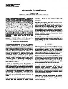
1.3.2 Embedded software: Embedded software: The software part of an embedded system is actually an embedded operating system. An embedded operating system is a special kind of operating system. An operating system manages the hardware of the computer and controls the operation of programs. It provides also an user interface which serves as a bridge for communication between user and computer. The operating system could interpret the instructions that the users give, so that the hardware could understand what they should do in order to achieve the functions. The main principles of the embedded operating systems are similar with a normal operating system. But its functions and operations are customized for the devices. It has generally fewer functions than a normal operating system and has a different user interface. According to [Shi], the operating system can generally be classified into three categories: order execution operating system, time-sharing operating system and real-time operating system. In an order execution operating system, there could be only one program in the system. This program occupies the whole CPU itself. In the time-sharing operating system, there could be more programs in the system. All the programs share the CPU. In a real-time operating system, there could be also programs in the system. Each program has a priority, only the task with the highest priority could occupy the CPU. We often use a real-time operating system in an embedded system. A realtime operating system can support multi-tasking, it organizes the sequence of the tasks according to a plan. Each program must be finished in a certain time frame. Users need not to adjust the sequence manually. The programs run automatically. So the operation of the system becomes easier. Because of
6
1.4 Application fields
the advantages of better support of multi-tasking and the easy operation, so it could be widely used in the embedded system. According to [Mar10], a realtime operating system could be still classified into two categories according to the real-time constraints: hard real-time operating system and soft realtime operating system. A hard real-time operating system means that, if a program could not be finished in a certain time frame, the system will result in a serious consequence. For example, every process in a flow line machine must be finished in a set time, or the product will be scrapped. You can change this set time, but the process must be finished on time. The other real-time operating systems are soft real-time operating system. They are more flexible, they could tolerate some occasional time-out errors. Developers could choose which realtime operating system that is more suitable for the application according to demands. Figure 1.1 shows the structure of ES briefly.
Figure 1.1: the composition of an embedded system (according to [Rui])
1.4 Application fields Embedded systems have already covered a huge range of applications. We enumerate some concrete application fields in the daily life. • Consumer electronic products Embedded systems have been most widely applied in this area. The products in this field are the most common products in our life. For example, a mp3 player and a mobile phone. The embedded system is the core member in these devices. Programs have been defined in embedded system in advance. The equipment can run the functions when it receives the command. In a mp3 player, it could control the play of music. You can easily push the “next” or “back” button to play a previous or next song or steer the “volume” wheel to control the volume. These operations are actually
7
1 Fan Zhuosi: Introduction to the ES the instructions that you give. Embedded system could tell the hardware what to do after executing the instructions. A mobile phone has generally more functions than a mp3 player. Most handy phones have already intergraded mp3 function. So they usually have a more complex embedded system. You may bring two or three such products with you when you go to school or go to work. Another good example is a washing machine. Now the operation of a washing machine has been strongly simplified. You can just easliy choose the function on the control panel what you want to wash, and then the machine could do the program automatically. All these programs are controlled by inner embedded system. • Manufacturing equipment The example is a production line. An embedded system could help it to control the processes. The production of a product could be accurately divided into several steps. An embedded system will control what should be done in which step. More importantly, it could enhance the accuracy of the production process, so that each end product could get the same quality. The application in this field makes the massive manufacture of a product in a short time become possible. • Automotive All the electronic equipments in a car are controlled by embedded systems. The automatic air-conditioning system could adjust the temperature automatically. The media system could achieve the functions of playing music, GPS navigation, rear camera display and so on. More importantly, some system could save your life in the emergencies. For example, the esp system. It could detect which tire loses the grip and then take the appropriate measures to ensure that the car is not out of control. A car is something that is armed by electronic equipments which are controlled by embedded systems. • Public management Embedded systems are usually used in the public management as well. The traffic system could tell you when you can go across the street, when you must wait. The video surveillance system could record and upload the videos automatically. Now these two systems are always intergraded into one combination system to manage the traffic. When something happens, the police could easily find the videos.
1.5 Problems We talked about lots of the advantages of embedded systems. They have also problems. The problems come from two aspects: the side of developer and the side of use. For the developers, they have to design both the hardware and software parts of a device. That makes more difficulty in the development. For the users, they could not upgrade or make changes to the embedded system themselves. If the system gets into trouble, the problem could only be solved
8
1.6 Conclusion by technical staff. But in general, the advantages of embedded systems far outweigh their disadvantages.
1.6 Conclusion This paper began with the definition of an embedded system. And then introduced the differences between a personal computer and an embedded system so that we could have a concrete conception of embedded systems. It also summarized the characteristics of embedded systems so that they could be widely used. The structure of the embedded systems have been divided into several components. The functions of each component have been defined. In the last two chapters, we presented some application fields of the embedded systems and also problems. This paper explains the importance of the embedded systems. With the development of embedded technologies, whey will be more widely used in the future.
9
1 Fan Zhuosi: Introduction to the ES
10
2 Johannes Muhr: Cyber-physical Systems 2.1 Introduction In the past decades the information and communication technology (ICT) has developed in an unbelievable velocity. In the middle of the nineties, many people probably didn’t know much about the Internet, maybe never heard of it at all. Nowadays, a life without Internet and the correspondending ICTs is unthinkable. In industraial countries, everybody comes in contact with different kinds of ICTs in daily life, as it is meanwhile in nearly ever product or used in services like the energy supply [BBB+ 10]. Thus, Embedded Software was developed further with a similiar speed, using technologies of ICTs. Embedded Software exists in small, daily used systems like a washing machine and smartphones, but by now also in larger systems (vehicles) subsist a lot of small embedded systems like in the antilock brake system (ABS) or in the electronic stability program (ESP) [Mar11]. Consequentially the market volume of embedded systems achieved in the year 2010 already an amount of 19 billion [BBB+ 10]. The next aim of the scientists is to create Cyber-physical systems (CPSs), an advancement and connection of Embedded Systems (ES). This work deals with that new topic. Section 2.2 explains the development of CPSs and its basic architecture, Section (2.3) deals with the challenges of CPSs during the process of creation. In the last part, Section 2.4, some modelling techniques and ways that lighten the design process are addressed.
2.2 Cyber-physical Systems In the first part of this work, the question “what do you understand under the term CPS and how has it developed ?” is answered. It starts with the development of CPSs, afterwards the term per se and also the structure of these Systems is explained. At the end of this part, CPSs are compared with the traditional Embedded- and Real-Time Systems and the visions and main benefits of CPSs are announced.
2.2.1 The development and concept The term Cyber-physical System (CPS) is a quite new notion in modern sciences. It emerged around 2006 in the National Science Foundation in the United States [LS11].
11
2 Johannes Muhr: Cyber-physical Systems
Figure 2.1: Evolution of Cyber-physical Systems
Figure 2.1 ([BGC+ 11]) shows the evolution process of CPSs. The process started with the evolution of small Embedded Systems (ES). Those traditional ESs were small single systems which combine physical processes with computing. But many of these ESs just replace mechanical work. Over time, new techniques and simultaneously better systems have been developed. The result was a networking of some different ESs which communicate with each other. Now, modern systems like automobile engine controllers can’t be simply replaced through mechanical devices anymore [BGC+ 11, Wol09]. The question is, whether these networked ESs can be seen as CPSs. That is not easily to be answered, especially as the German BITCOM uses CPS as a synonym for ES [BBB+ 10]. So in the view of the BITCOM, CPSs are just common systems, which are already available. On the other side, the National Science Foundation (NSF) clearly differs between the two terms and says that CPSs are not the “traditional post-hoc embedded/real-time systems and not today’s sensor nets” [Gil08]. So, the NSF recognizes in CPSs a larger dimension than it is the fact in the common ESs. To consolidate these facts we say that the networked ESs of today are a kind of “small” CPSs. But the actual meaning of the NSF was different. This concept will be explained in the following section. Due to the huge scope of the term several definitions are used. The following two examples express the fundamental factors of CPSs. “Cyber-Physical Systems (CPS) are integrations of computation with physical processes. Embedded computer and networks monitor and control the physical processes, usually with feedback loops where physical processes affect computations and vice versa.” [Lee08]
12
2.2 Cyber-physical Systems
“Cyber-physical systems (CPS) are physical and engineered systems whose operations are monitored, coordinated, controlled and integrated by a computing and communication core.” [Sta10] As we can see in these two definitions, the key point of CPSs is the two way interaction between physical laws and computation. In CPSs, these sciences are not united, but rather intersected. Instead of concentrating on single topics of the system, we should focus on the interaction of them. Figure 2.2 ([LS11]) illustrates an abstract example of the structure of CPSs. Especially the interaction of the individual elements from the different components is clearly shown [LS11].
Figure 2.2: Abstract structure of Cyber-physical Systems
There are three main parts in this illustration (Figure 2.2), the first part is the physical plant, which is simply everything that is not realized with computers, it can include various things like mechanical parts and so on. The second part involves one or more computational platforms with components like computers, sensors and actuators. Sensors measure the results of the process and actuators impact on base of the elaborations on the physical plant. The last part is the communication (network fabric), which provides the communication mechanisms for the computers of the different platforms. The ICTs provides different ways to execute the data communication in the network fabric. Together, the network fabric and the computational platforms form the “cyber” in the term Cyber-physical Systems, whereas the physical plant stands for the “physical”. In this example (Figure 2.2), there are two platforms, each platform has one sensor measuring the impact of the physical processes. The platform 2 includes an actuator that controls the physical plant. Computation 1 sends the measured data via the communication network (network fabric) to computation 3.
13
2 Johannes Muhr: Cyber-physical Systems
Each computation element implements a control law giving commands to the actuator, based on the data received from the sensors. So the commands of computation 2 and the consolidated commands of computation 1 and computation 3 are merged and sent to the actuator. Together, the structure of CPSs is characterised through the complicated interaction and connection of Embedded-, Computational Systems with (worldwide) networks. CPSs can communicate with communication platforms like the Internet with widely distributed systems. To be more generally, CPSs are the intersection and the direct connection between the physical and digital world. Though, the digital world involves various components like the communication medium, computers and so on [Bro10].
2.2.2 Classification We have seen in the first section (cf. 2.2.1) that it is often difficult to classify the different Systems to their belonging. We learned also something about the special characteristics of CPSs. In this section, CPSs are classified in the overall context and challenges of this classification are introduced and discussed. Figure 2.3 ([Bro10]) shows the architecture of CPSs, where we can see that a major part of them is built up on ESs and all the corresponding components like: sensors, actuators, hardware, software and also the interfaces to users and further systems.
Figure 2.3: The Architecture of CPS
Therefore it is sometimes not easy to conclude if a system is still an ES or already a small CPS. Figure 2.4 illustrates again the large overlap of Embedded-,
14
2.2 Cyber-physical Systems
Real-Time (RTS)- and CPSs1 . It is clear that there is an overlap between CPSs and ESs as each CPS needs embedded software to work and integrates computation with physical processes. But the difference to the traditional ESs is that CPSs do not simply replace mechanical work and they have the focus on a multitude of devices. Together, CPSs are more distributed and more interactive with the nature [Bro10, KKI+ 11, Wol09]. In comparison to the modern ESs, CPSs work and communicate in a very large system, whereas the ESs are within a well-defined system. An example is the mentioned automobile engine controllers (ES, “small” CPS) in a car. An example for a CPS would be a networked intelligent intersection, where a set of cars are communicating with each other. Additionally, the cars can access to detailed information from the infrastructure and the other way round. The task of the whole system (cars, traffic lights, etc.) is to arrange an efficient traffic flow in real time. For example the system must notice if there are a lot of cars waiting in front of a traffic light. Then it should try to dissolve the jam as soon as possible in consultation with the other elements of the system (other cars and traffic lights) [Gil08].
Figure 2.4: Overview of Embedded-, Real-Time- and Cyber-physical Systems
In comparison with Real-Time Systems (RTSs), it is again obvious that CPSs have tasks that must be executed periodically or that they have deadline or latency constraints. But the difference is that in the classical field of RTSs, the system does not interact in the process from itself. So the system monitors the action and may give some signals, but it does not try to solve the problem itself. In the last example with the intelligent intersection (cf. 2.2.2) we have seen that CPSs should try to find its own answer. Examples for classical RTSs are monitoring consoles in hospitals. They supervise certain values and give alarm if a critical limit is reached; still they do not interact in the process and do not help the doctor to reduce the increased magnitudes [LCS+ 88]. 1
Figure at the address http://scm-l3.technorati.com/10/02/03/4111/cps-technorati. jpg
15
2 Johannes Muhr: Cyber-physical Systems
2.2.3 Vision and Aims In this section the focus lies on the actual vision and goals of CPSs. The intension of CPSs is to create a huge network with distributed systems that can interact and communicate with each other and with humans through new modalities. Based on the new abilities of interaction with the physical world, the high functionality and reliability; CPSs will be a key enabler for future technology developments that far exceed the levels of autonomy today [BG11]. That results in the area of automotive as an extensive network between all vehicles and the complete infrastructure, like traffic lights or parking decks. Due to the continuous real-time data exchange (about weather, information about the traffic, etc), the distributed traffic management systems can work as a planning and coordination assistant and react on unforeseen situations like traffic jam. Through an optimal traffic management with an early recognition of threats and barriers, the road safety (less accidents with other cars or passengers) may be increased. Further, through this intelligent planning the road users may save time and money due to the reduction of fuel consumption and the CO2 saving, which is also important for the environment protection. The grand vision of Cyber-physical System is the Smart City [BGC+ 11], which is a cross domain topic which involves different sectors, like smart mobility, smart health, smart grid, smart factory, smart home and so on. These sectors are all connected with each other and manifest a lot of interdependencies. An example for the combination of smart home and health is a system that recognizes and gives an alarm signal, if a room is (for a defined amount of time) empty and the stove is on. So, the different future scenarios are not isolated from each other, instead-, there are a lot of relationships and dependencies between the distributed subsystems.
2.3 Challenges We have seen that CPSs are very complex and large systems, with a wide range of applications. It includes the mentioned traffic control, safety and advanced automotive systems, avionics, environmental control like the observation of water resources, infrastructure control, communication systems, electric power and so on. Altogether, most applications are safety critical or at least critical in that each system affects other areas [Lee06]. So it is obvious that the design and modelling of these systems is very challenging. Some of the challenges that arise during the design process of CPSs are introduced and discussed in the next sections.
16
2.3 Challenges
2.3.1 Non-functional Challenges It is very important that CPSs meet the dependability aspects (reliability, maintainability, availability, safety and security) to guarantee a save use of the system. The reliability, so the probability of failing, must be limited to a value near zero, since most systems are critical. As this is not 100% guaranteed, the failing system must be repaired in a minimum time-frame (high maintainability) so that the negative effects through the failure of the system (damage, costs, etc.) are as small as possible. The reliability and maintainability should be high in order to fulfill a high availability. The property of causing any harm through a system failure must be again very low (high safety). The challenge and risk of CPSs is that even small errors can lead to enormous damage and an endangering of human life. For the same reasons, but also in the interest of data protection, it must be guaranteed that the confidential data of the systems stays conversant. In equal measure, the system must be protected from hostile takeovers (high security). This is again a very demanding challenge as the systems are very large and interact with each other; therefore there are a lot of possibilities to influence the process in a malicious way [Mar11].
2.3.2 Digital and analog world An elemental problem of CPSs is the gap between the digital and analog world. While the physical part is based on the classical continuous math, the digital information processing (which involves models for the implementation, pattern for data acquisitions, processes and architecture of the digital systems) is based on discrete logic. But through the interaction of the physics with computation, CPSs must consolidate two (from the origin) very different domains. Models that constrain themselves to only one of the two approaches (digital or analog) are in those cases useless. Therefore, there is a need of an integrated systemand model-layer, which combines the diverse mathematical ways. To join the indivudual models (digital and analog), qualified levels of abstraction have to be found. A model which is able to consolidate the analog and digital domain is called Hybrid-System [HKPV98, Bro10] (cf. Section 2.4.3).
2.3.3 Complexity Challenge A further problem is the environment that interacts with the systems. Physical processes are by nature concurrent, which means that there are parallel processes. An additional difficulty is the fact that these processes cannot be exactly foreseen [Lee06]. Even if a system is engineered reliable and predictable, the nature can still manage to expose the system to an unknown condition. CPSs are working consequently in an uncontrolled environment. As a result, CPSs must be adaptable to failures as the availability can never be absolutely guaranteed [Lee08], although this is very difficult, since a lot of systems are interdependent and need data from each other to execute perfectly.
17
2 Johannes Muhr: Cyber-physical Systems Further, due to this networked environment and the combination of different disciplines like computer science and electrical engineering, all standard engineering methods become more complicated. Based on the dimension of those systems, different modelling techniques from different branches are used that are not directly compatible and suitable. Divisions of labour and decentralized working are further keywords that complicate the engineering process relevantly [Bro10]. Consider the smart city that was introduced in Section 2.2.3, it is very difficult to arrange the interdependencies and the involved developers in the modeling of the system. These properties and conditions influence the whole engineering process. At the end of this process there is once again a huge challenge. Testing the major network with all the different subsystems seems to be very challenging [Lee08].
2.3.4 Lack of Timing Another challenge of CPSs is the software part. A simple programm with no concurrency can perform on a computer with 100% reliability, but in CPSs there are instead of small programms huge software systems. Keeping this software (or rather the software model) in that complicated dependency consistent is a big challenge. A further problem are the high interconnected sensors and actuators. In CPSs the interaction between sensors and the hardware of actuators (cf. Section 2.2.1) is very important, but this specific behavior is not very well represented in programming languages. The problem is that imperative or sequential programming languages do not match well with the needs of CPSs. Even the simplest program is in the context of CPSs not reliable, as the aspects of the systems behavior are not expressed by the language. It can execute perfectly and match all semantics, but it can still miss real-time constraints, because timing is not in their semantics. But meeting this real-time constraints is essential for CPSs. This is an issue from the very first time in the development process, where the concurrent processes must be known and illustrated in models. This problem becomes more complex and worse if the systems get bigger and bigger, as it is the case with CPSs [DLSV12, Lee08, Mar11].
2.4 Modelling techniques The challenges discussed in the last section (cf. 2.3) show the huge amount of problems that need to be overcome. In the next section, some models and techniques, which help and simplify the modelling process, are explained.
2.4.1 Models of Computation In Section 2.3 it is mentioned several times that a lot of the problems emerge from the heterogeneity and complexity of CPSs and their applications. To relieve that problem in the design process, qualified levels of abstraction have to
18
2.4 Modelling techniques be found that use modelling techniques with well-defined, expressive and precise semantics. This can be fulfilled with the Model of Computation (MoC), which is a defined set of operations used in computation and their respective costs. There are a variety of such models existing (Turing machine, finite-state machine, random-acess machine and so on), so it is usually not easy to find a suitable model. Especially the heterogeneity of CPSs forces the developer to combine a multiplicity of models. In the case of CPSs, the MoCs try to illustrate the concurrent composition of actors. An actor is a component that reacts to stimuli at input ports and produces stimuli on output ports. The interaction of the actors is defined by three sets of rules. The first set specifies the constitution of the components, which means having an overview about the whole architecture of the systems from the beginning, knowing which systems are dependent and affect each other. Secondly, you have to specify the concurrency mechanisms. After knowing the interdependencies of the subsystems you have to determine how the systems give semantic to the concurrency. For example, define whether the systems execute simultaneously or if they share a notion of time. The last set of rules defines the semantics of the communication mechanism. Specifying, if the subsystems communicate via synchronous or asynchronous messages or which protocols for the data exchange are used and so on. The challenge in the design process is to identify the actually needed MoCs from the huge amount that is available [DLSV12, LS11, Sav98].
2.4.2 Multimodelling It is already mentioned in this work that interfaces are the key issue for CPSs (cf. Section 2.2.1). Through the magnitude and heterogeneity of CPSs and the resulting work-sharing processes, a lot of different modelling and specification techniques are used during the design process and further actions (various MoCs). The problem is that the semantics of the different MoCs are not directly compatible and comparable. So the main focus should lay on the integration of the multiple models to get the interfaces operating with each other. This is called “multimodelling”. Good software architecture for a CPS and their interoperations will only arise from an excellent and errorless understanding of the semantics of interoperation (cf. Section 2.4.1). Further, the deterministic aspects of elaboration must be a very important property of these systems, especially through the huge amount of interfaces to other subsystems. A particular input must always lead to the same output in all dependent systems. Otherwise, the requirements of the non functional challenges (cf. Section 2.3.1) could not be achieved, as the system has no operation mode that leads to a reliable output. Non-determinism is only used if it is needed by the application. Through this kind of modelling, better concurrency mechanisms than with the normally used models and a better interoperation are possible [DLSV12].
19
2 Johannes Muhr: Cyber-physical Systems
2.4.3 Hybrid Systems CPSs are the integration of computation, networking and the physical dynamics. Therefore, single models (cf. Section 2.3.2) that address only either to differential equations (continuous dynamics) or to state-machines (discrete dynamics) are in that case inadequate. Hybrid systems try to deal with this problem by providing a bridge between the state-machines and the time based models. The notion stands for a particular composition of continuous and discrete dynamics. In other words, the systems proceeds continuously, but has occasional jumps, corresponding to the state change in an automata. These transitions are caused either by the continuous evolution itself or by external events (stimuli on the input ports). A very trivial example from [LS11] is a thermostat, which has no continuous state variables, no output actions and no set actions (cf. Figure 2.5).
Figure 2.5: A thermostat with continuous-time output
Instead of a discrete input, the system receives a continuous time signal (Π (t)), the temperature at time t. Further, the thermostat has the two states, cooling and heating, whereat each state is associated with a time-based system (a so called state refinement labeled as “h(t)”). In a hybrid system, the current state of the state machine gives the dynamic behavior of the output (h) as a function of the input (Π). In the example, the system produces a signal whose value is 0 when the heat is off and 1 when the heat is on. Such control signals could directly supervise the thermostat and drive it.
2.5 Conclusion We have seen in this work that CPSs compromise models of physical processes as well as models of the software, computational platforms and networks. For developing CPSs the existing technologies are sufficient. They need new ones that combine the different models of CPSs and overcome the challenges. Although
20
2.5 Conclusion in the meantime some tools that relieve the design process were developed, it is still a long way to develop dependent and large CPSs, but in foreseeable time physical computing will interact more and more in our life and will revolutionize a lot of areas like transportation systems, manufacturing, process control and power grids. There are already projects existing (for example project simTD in Germany) that explore and prove technologies like the car to car communication (like in the mentioned intelligent intersection (cf. 2.2.2)) and applications for a save and intelligent mobility. Altogether a save application of CPSs will lead to a more efficient and saver life for people all age groups and can also protect the environment [Sta10], as explained in this project 2 .
2
www.simtd.de
21
2 Johannes Muhr: Cyber-physical Systems
22
3 Christian Lichtmannegger: Real-time systems 3.1 Introduction Real-time (RT) systems are an important field in embedded systems and embedded systems are an important part of our daily life. This is called ubiquitous computing. It is no surprise when a person has 2 or more computers and if we count the embedded systems too, then people can easily have 10 or more. RT systems make a big part of embedded systems and therefore a big part of our life. A RT system produces a result in a given time interval. Because the aspect of time is mostly excluded in the majority of programming languages, so it is hard to make time itself part of your program. In addition, normal operating systems give a very good average efficiency but a RT task must finish in time, so the scheduling must be changed, to fulfill the timing aspect [Sta96b, YB+ 97]. Only those points show that RT systems can be a very interesting field of research. In this paper, I will examine some fundamental aspects of RT systems and show you some techniques to overcome the scheduling problems.
3.2 The basics There are various definitions of RT systems but I focus on the one proposed by John A. Stankovic [Sta96a]. “Real-time systems are those systems in which the correctness of the systems depends not only on the logical result of computation but also on the time at which the results are produced.” We can reduce this quote to two key messages. Logical result That means if the system solves the problem or not Time aspect That means how much time does it take to get the logical result So we do not only have to focus on solving the problem, but we have also to consider how much time does it take. For instance, because if you sit in a car and have an accident then it is necessary not only that the airbag opens but also that it will open in time. This shows very well that RT systems can be safety critical [BLMSV98]. To get a better understanding of what RT systems are, I will give three examples of them. Table 3.1 shows three different examples of RT systems. They have some common but also different aspects. All RT systems consist of a controlling part, that is the computer chip and the RT system itself, and a controlled part. That is the environment the computer interacts [Sta96a]. In case of
23
3 Christian Lichtmannegger: Real-time systems Air-traffic control
Assembly lines in in- Remote conference dustry application Consist of a controlling and a controlled system Scheduling of processes to meet the RT constraints Hard RT constraints Hard and soft RT con- Soft RT constraints straints Safety critical system Less safety critical sys- Not safety critical system tem Figure 3.1: Examples of different RT system
the air-traffic control system the environment are the planes and the airports. In case of the assembly line example the environment is defined through the assembly line itself and in the example with the remote conference application the environment are the users of the system and their PCs. But thats nothing special because this pattern of a controlling and a controlled system is caused by it’s definition as an embedded system. Every embedded system consists of this two part. So RT systems are embedded systems by their definition. The next common point is the importance of scheduling processes. This is exactly the second point given by the definition at the beginning of this article. The time when a result is produced is important. All RT systems have a special scheduling algorithm and I will examine some of them in the following chapter. Despite those common points this systems have many differences too. Not to mention the different costs of an air-traffic control system and a remote conference application there are fundamental differences like safety criticalness. There is a strong relation between timing constraints and the safety criticalness of a system. You can use this simple thumb rule: The more safety critical the system is the harder are the deadlines of the tasks. Every task has its own deadline but it possible to miss the deadline in some case. If this is possible the deadline is called soft if not the deadline is hard (cf. [BLMSV98]). In the example of an air traffic control system the deadlines are hard because the pilots need all the information in the right time to react and prevent a disaster. In assembly lines the deadlines are largely soft because if a task can not be executed in time then the system can reduce the speed of the assembly line to give the tasks more time to finish. The problem with that is that if the system often reduces its speed, you can produce less goods and therefore the rate of met to missed deadlines is an important mark of quality of those systems. In a remote conference application you have only soft deadlines because problems are just only annoying, if you hear a bad noise or see some skipped frames on the monitor, for example. But here also the rate of met and missed deadlines plays a role in quality (cf. [Sta96b]).
24
3.3 Scheduling
3.2.1 Different types of tasks It’s important to know that in a RT system you have to handle different types of tasks: Periodic task This is the most simple task. Its deadline just repeats itself after a periodic time interval. So this task must be executed every n time units. Aperiodic task This task has to be executed after an event occurs. So its deadline is defined through the time the trigger event occurs. Sporadic task This task is quiet similar to an aperiodic task. The main difference is, that between two activations of a sporadic task a given time interval must have been passed. That means that after the first execution of the task you must wait until this interval passed before you can activate the task a second time.
3.3 Scheduling 3.3.1 Scheduling: The basics Schedule is the process of allocating resources to various tasks. The main resources in computation systems are CPU resources and computation time. So you allocate a task to one or more specific CPU units for a specific time. The problem is that, in most cases, we do not exactly know how long it takes to execute a task. So we need a reference value and this is the worst case execution time. Because when you know, that a task takes between n and m time units, the task is definitely finished after m time units. So you can guarantee to have enough time for execution whatever happens. So a task is not only defined by its deadline, like in the above text, but also by its worst case execution time. To make it simpler I assume that a task always takes all the resources of a CPU, so only one task can be executed on the same CPU at the same time. Scheduling in RT systems must meet two goals: 1. Meeting deadlines 2. Maximize resource utilization The first point, that a RT system must meet its deadlines is essential and the key objective. But you have to think about resource utilization too. Those two goals often conflict each others. Because if you have so much resources too meet all deadlines whatever happens, then you normally have a very low resource utilization. This means that you have much unused CPU space and this makes the system more expensive. On the other hand, if you have a very high resource utilization then you have only few unused CPU space and if you have to execute an unexpected task you can not execute it. So you must find a good balance between those two key objectives (cf. [BLMSV98]). There are two different approaches to meet those objectives. Static and dynamic scheduling.
25
3 Christian Lichtmannegger: Real-time systems
3.3.2 Static scheduling Static scheduling is to form a feasible schedule before runtime. That means that all the computation effort for scheduling is done before runtime and so less computation resources are needed during runtime. That makes the resulting system much cheaper. 3.3.2.1 Round Robin/Static cyclic scheduling The most basic algorithm is called Round Robin. At the beginning there is a task pool and we just form a cycle from all those tasks. So we have a cycle with every single task in it. During runtime the tasks of the cycle will be checked if they can be executed. That means that there are enough resources free to execute it. If a task can be executed then it will be started immediately. Else the next task will be checked. This algorithm does not care about deadlines and the only good thing about it is that every task is checked once in a cycle but it could happen that important tasks must wait very long until execution (cf. [BLMSV98]). Pro • Very low memory allocation
Contra • Many deadlines could be missed
• Every task is checked during a cycle
A little improvement of the standard Round Robin approach is to duplicate important tasks, so they appear more often in the cycle. This little change seems to reduce the missing deadlines problem significantly but it also increases the cycle length. The result is although important tasks are checked and executed more often the ”normal” tasks lack of execution. In addition it takes longer to go through the cycle so the execution problem is increasing too. Pro • Very low memory allocation • Increased number of checks for important tasks
26
Contra • We can not predict that all deadlines will be met
3.3 Scheduling
Figure 3.2: Cyclic algorithm every LCM
3.3.2.2 Cyclic static table driven algorithm A very efficient algorithm is a cyclic algorithm which repeats every least common multiply (LCM) of the task length. If there are tasks that take 10, 20 and 30 ms of worst case execution time, then the LCM of those tasks is 60 ms. So the scheduler forms a cycle length of 60 ms. Now the scheduler looks at the deadlines of the tasks and tries all permutations of those tasks, so they are all finished in time. If the scheduler finds a proper schedule, then the work is done. This cycle is repeated continuously during execution time of the system. An example of this technique is shown in Figure 3.2. If the scheduler can not find a feasible schedule then more CPU resources must be added. In case of a very long task, the scheduler can split this task into independent subtasks, to get a better usage of the resources. Those subtasks can be executed on their own and at the end of computation the results are put together to form the final result of the task. This is only possible if a splitter tasks does not need information from another splitter task to continue. It could happen that there is some unused computation time at the end of the cycle and if that is the case it could be possible to reduce the number of CPUs to get a better capacity utilization. Because in worst case the scheduler must check all permutations of tasks to find a feasible schedule and additionally he can split up tasks and make even more tasks, the computation effort for creating a schedule is growing exponentially. The good thing is that all that effort is done before runtime. That results in less wasted computation resources during runtime and so the system is much cheaper then one with dynamic scheduling. Because during one cycle, no deadline is missed and the cycle repeats in a static way it is easy to predict, that no deadline will be missed. So it’s perfect for safety critical issues (cf. [BLMSV98]).
27
3 Christian Lichtmannegger: Real-time systems Pro • Very predictable • Splitting of tasks increase feasibility of schedules • Good for safety critical systems
Contra • Very high computation effort before runtime • Splitting of tasks increases the effort even more
3.3.2.3 Analysis So in fact good static algorithms are very predictable. So all deadlines will be achieved and they are mostly used in safety critical systems. Because we can guarantee that the system will not miss a deadline. Another good point is that all the computation effort is done pre-runtime and so the resulting system needs less computation resources. A problem with static algorithms is that it is hard to implement aperiodic tasks and user interaction. The predictability of such a system is caused by the knowledge when a task arrives. If there is an aperiodic task, you do not know when it will start and so you do not know the exact deadlines pre-runtime. It is likely the same with user interactions. It would be possible to make an extra slot just for those unpredictable tasks but if you have an overload of tasks, so you can not execute all of them in time then a static system fails. Another problem I totally ignored in this article so far, is that tasks could fail. It could happen that through a programming mistake or just a bit switch, the task fails and the result of the computation is useless. To overcome these problems dynamic algorithms were created.
3.3.3 Dynamic scheduling The main difference of dynamic by comparison to static scheduling is that the creation of a feasible schedule is done during runtime. That means that CPU resources are needed to create the schedule. So the chip makes continuously feasibility checks. That means extensive simulations and requires the use of heuristic functions to keep the effort acceptable. Another difference to static approaches is the use of a dynamic priority. So every task has a worst case execution time, a deadline and a priority. If there is an overload, that means that there are so many tasks that not all of them can be executed punctual, then a task with a higher priority is privileged. The concept a priority can be used in static techniques too, but in dynamic scheduling algorithm the priority can change. So it is more flexible. The problem with dynamic algorithms is that most of them are very complex and so I will only show very simple and basic ones. A more complex and efficient algorithm is described in (cf. [MM98]).
28
3.3 Scheduling
Figure 3.3: Task Pool
3.3.3.1 Least laxity first (LLF)/Dynamic earliest deadline first Two basic algorithms are LLF and DEDF. They are both priority driven algorithm and their priority is calculated very simple. LLF has the laxity as priority. Laxity is the amount of time a task can wait before starting the execution, so it will still meet its deadline. At first there is a task pool and the scheduler creates a priority queue with the task with least laxity first. Then the tasks are assigned to CPU resources one after another. If there are multiple CPUs then it is possible to execute more tasks at a time. The change of priority is pretty self explaining, because as time proceeds the laxity of all tasks decreases. If there is another task, then it will be added to the queue properly.
Figure 3.4: The resulting schedule DEDF is pretty similar to LLF, the only difference is the priority here is just the time until the deadline arrives. That reduces the calculation effort for priority but it is almost only used in systems where all tasks have the same execution time. Because then the computation time is irrelevant for the priority (cf. [BLMSV98]). 3.3.3.2 The problem with overloads I already mentioned in the introduction to dynamic algorithm, that an overload is when there are so many tasks that some of then cannot be executed in time. Then the algorithm has to differ between tasks that are worth to execute and those that can be discarded and execute later. That means that safety critical tasks like opening an airbag has a high value and controlling the air conditioner for example has a low value. Or the length of the execution time reduces
29
3 Christian Lichtmannegger: Real-time systems value, or soft real time constraints reduce value, while hard deadlines increase it (cf. [BLMSV98]). 3.3.3.3 Fault tolerance Another big advantage of dynamic systems is that they are fault tolerant. It could happen that through a simple bit switch or a programming bug, the task fails and the result is useless. The key idea behind fault tolerant systems is that you have two tasks, to solve the same problem Primary task This task is scheduled that it will meet the soft deadline of the task or so that a secondary task can be executed before the hard deadline arrives. This task is normally sufficient. Secondary task This task is like a backup, it is scheduled directly after the primary task. This task is only executed if the primary task fails. That means that if no error occurs the secondary task is discarded and if there is an error then the second task solves the problem in time. It is also possible to use more then one backup task. But this means that there is a huge waste of resources, because if the secondary task is discarded in most cases then this time is lost for other task. To solve this problem it seems logical to use resource reclaiming too (cf. [BLMSV98]). 3.3.3.4 Resource reclaiming Resource reclaiming goes hand in hand with fault tolerance in most cases. But systems without backup tasks use it as well. Because the scheduler assigns a task for its worst case execution time to a CPU, a task normally ends before it reaches its worst case execution time, so almost every task wastes resources. This is a problem and dynamic scheduling gives us the opportunity to change this. A system that uses resource reclaiming uses this unused computation time to run RT or non-RT tasks. This rescheduling must be very quick so it takes only very little time to reschedule tasks. It is important to predict that if we save time, the computation effort to reschedule is lower then the saved time, independent from the number of tasks running. 3.3.3.5 Discussion The main disadvantage with dynamic scheduling systems is that they do not exactly know when a task arrives. So it is hard to promise that all deadlines will be met and due to the extra CPU the system is more expensive too. But for systems with high user interaction static approaches do not fit and dynamic algorithm evolved in the past years so they are a very good alternative. Especially resource reclaiming and fault tolerance increase their efficiency dramatically. But this algorithms, are very complex, image an overload and you discard some tasks, then you do not need a secondary task and save computation time then it could be possible to reschedule discarded tasks then simply move all other tasks forward.
30
3.4 RT operating systems
3.4 RT operating systems Most systems need an operating system (OS) to work properly, but “normal” OS do not fit RT requirements. They offer a good average performance but in RT systems there is a need for higher priority for hard RT tasks and a lower priority for all other tasks. So a new type of special purpose OS are invented, RTOS. They offer the same functionality of normal OS • Process management • Memory management • Interprocess communication • In- and Output RTOS can be divided into 3 main categories: Small and fast kernels, RT extensions for existing OS and research kernels. Small and fast kernels are those chips you find in most RT systems. They are cheap and like the name says they are small. This results in reduced functionality, compared to a normal big OS, but they respond to interrupts quickly and minimize the time between intervals those interrupts are disabled. Those points makes those kernels very fast. But fast is not RT, so they maintain a real time clock, for synchronization and they support real time queuing. Many also provide a priority scheduling mechanism. All this together turns the system into a RTOS (cf. [HP88, BLMSV98]). RT extensions for existing OS are a new approach to bring the RT part into a normal OS. The problem is that writing a new OS with all the functionality of Windows or Linux would be exhausting and so RT extensions were created. For example RT Linux, it is just a small application inside of Linux. If there is a non-RT process, then nothing special will happen and Linux will take care of this process. But if a RT process arrives then RT Linux takes over control. To reduce the complexity of RT Linux it will only take care of the RT part of the task, so almost all RT tasks will be split into a RT and non-RT part. The non-RT part will be executed by “normal” Linux and also scheduled by Linux. The in most cases very small RT part of the task will then be handled under RT conditions. As example we can imagine an audio recording task. This process consists of two main parts, storing the RT stream in a buffer and writing the buffer into a file. In this case storing the RT stream is the RT part, because this recording has to be done very accurate, to enhance quality, while writing the buffer into a file to save the record can be done almost at any time. So only a small part of the whole task is really done in RT and the rest is done conventional (cf. [YB+ 97]). Research kernels are experimental kernels to try out new ways of solving problems, or are specialized kernels for very specific tasks. Those kernels are out of scope of this paper.
31
Manuel Bonk: Tasks in Embedded Systems
3.5 Developing of RT systems Now we know what RT systems exactly are and how they work, but the developing of those systems is also an important field of research. RT systems feature the combination of soft- and hardware. That makes testing and verification harder, because not only the software must be checked but also the interaction with the hardware components. Additionally the size and complexity of RT systems is growing and this increases the effort for testing and verification even more. That makes testing and verification extremely expensive, especially for more safety critical system where more testing must be done. The idea to improve this situation is to make testing and verification a pervasive part of software development. Because the costs of repairing an error are increasing exponential compared to the time the error is detected. This would not only save money it would also leads to a better code. If an error is found early then a new solution can be created, but if the error is detected at the end then in many cases a complicated fix is done, which makes the system harder to maintain and to understand. At first an informal specification is given, this normally comes from the client. This can be transformed in a semi formal specification. This can be seen as an optional step, but is useful in many cases. A semi formal specification is normally given as pseudo code. This specification will then be transformed into a formal specification. Such a formal specification is given in a formal language, which can be proved through a proving software or by hand. This is the first check cycle, if the system fits the requirements or not. The next step is forming a model of the system and test and verify this model. If everything is correct then the final code will be created and will be checked one last time, before release. This new model implements three checking cycles and will probably be adopted by industry (cf. [HST10a, HST10b]).
3.6 Conclusion Now we have a good impression what RT systems are and how they work. RT systems cover a wide spread of fields of application, so their future importance will grow. Because of the separation between soft and hard RT constraints we are able to develop systems to satisfy different needs, like costs, flexibility, predictability or safety criticalness. Also the improvements brought to us by RTOS will find their way into “normal” OS too. But beside these points scheduling is still the main problem with RT systems and so this is a very interesting field of research, especially in the dynamic scheduling section. It would be great to find a technique to make dynamic scheduling more predictable so all their advantages could be used in safety critical systems too. All in all RT systems are very interesting and the more research is done in this field, the more persistent those systems will become. This effect will be boosted by ubiquitous computing. So RT systems in combination with embedded systems systems in general will probably have a very high impact on our daily life.
32
4 Manuel Bonk: Tasks in Embedded Systems 4.1 Introduction In our everyday life embedded systems become more and more important. Even if people often doesn’t recognize them as computer systems embedded systems are small units often dedicated for very few and specialized use cases only. Nearly every embedded system is controlled by a real-time operating system. These operating systems organize their workload by the means of tasks. It will be elucidated how tasks are realized in real-time operating systems for embedded systems in general and in OSEK OS and OSEKtime OS in particular.
4.2 Definition of Tasks The main part of this chapter, Sections 4.2–4.4, is based on the materials from [SZ10]. This chapter is organized as follows: first of all, in section 4.2 we give a definition of a task, then in section 4.3 processes are described. Section 4.4 is about the different kinds of interaction between tasks. First of all a task needs to be defined. Larger assignments can conveniently be subdivided in smaller parts. These parts can be implemented by the means of tasks. A task provides the framework for the execution of functions. The operating system is responsible for both task switching mechanisms and the concurrent and asynchronous execution of tasks. A task is executed after its activation. Timing is the most essential part of a real-time operating system. Therefore there are various time slots, one for each task. There are two kinds of real-time requirements a task has to fulfill: • “Hard” real-time requirements: at the end of a task’s execution time slot the result is validated with a short test. If this test fails an error is thrown, if not, the system continues with the next task. • “Soft” real-time requirements: the results of these tasks needn’t be validated after their termination. In order that tasks can be executed correctly a worst case execution time (WCET) has to be calculated and set. For more information see [SZ10].
4.3 Processes A set of tasks with equal real-time requirements can be handled as a set of tasks or can be summarized to a larger task. The subtasks of these larger tasks are
33
4 Manuel Bonk: Tasks in Embedded Systems
called processes (cf. Figure 4.1). The execution order of the processes has to be adhered and can’t be varied of the former order. For further information see [SZ10].
Figure 4.1: Process (adapted from [SZ10])
4.4 Interaction between Tasks Tasks are “parallel” (e.g. on a multi-core system) or “alternating/quasi-parallel” (cf. also [SZ10]) executed and most of them collaborate in a larger assignment they have to interact with each other. In the following the different types of interaction between tasks, such as Synchronization via Events, Cooperation via Global Variables and Communication via Messages are described. Not all kinds of information exchange always works properly. Therefore several errors could occur. In the following subsections possible errors are also elucidated.
4.4.1 Synchronization via Events The simplest form of interaction between tasks is the synchronization via events (cf. Figure 4.2 and also [SZ10]): a task sends a short event with very few information such as “the light is on” to another task. By receiving and sending an event a task changes its state. Because of this simplicity there are nearly no error sources.
4.4.2 Cooperation via Global Variables Another yet slightly more complex possibility of interaction between tasks is the cooperation via global variables (cf. Figure 4.3). An example for this procedure is visualized in the following: Task A initializes a global variable and assign a value to it. Task can access and process the newly created variable. Global variables contain more information than synchronized events. But with greater capabilities comes greater
34
4.4 Interaction between Tasks
Figure 4.2: Synchronization via events (adapted from [SZ10])
Figure 4.3: Collaboration via a global variable (adapted from [SZ10])
susceptibility to errors. For instance, Task A writes a global variable and simultaneously Task B reads said variable. Task B will get inconsistent data, as shown on Figure 4.4. This issue can easily be fixed the usage of an interrupt lock: If a task writes a value to a global variable no other task can read the variable while the writing task hasn’t finished writing (cf. Figure 4.5).
Figure 4.4: Inconsistency by simultaneous read and write access (adapted from [SZ10])
35
4 Manuel Bonk: Tasks in Embedded Systems
Figure 4.5: Read access is denied while a variable is written to (adapted from [SZ10])
In some case the cooperation via global variables is still error-prone. Put the case that Task A declares X := x1 . After writing the variable but before termination Task A gets paused and Tasks B is started. Task B reads variable X and uses the received value x1 for further computations. During these calculations Task B is interrupted and Task A is resumed. Task A now assigns X a new value x2 . After that Task A terminates and Task B is getting continued. Task B now needs to read X again for its computations. But now it uses the newly received value x2 which distorts the results, as shown on Figure 4.6. For a more detailed description see [SZ10].
Figure 4.6: Inconsistency after interruption of Task B by Task A (adapted from [SZ10])
4.4.3 Communication via Messages The most sophisticated mode of interaction between tasks is the communication via messages (cf. Figure 4.7 and also [SZ10]). This mean of interaction is very similar to the cooperation via global variables. If a task receives a message containing a value x1 assigned to variable X a local copy is made. Task B
36
4.5 Tasks in OSEK-OS and OSEKtime OS
makes a local copy of the received variables. If tasks B needs the variable again the locally copied the local co the received variable X is used the locally saved x1 is read. If during the task’s execution a message containing a reassigned variable X is received it will be ignored. Due to that strategy consistency between input and output is maintained.
Figure 4.7: Synchronization via messages (adapted from [SZ10])
4.5 Tasks in OSEK-OS and OSEKtime OS In the previous paragraphs tasks we discussed the behavior of tasks in general in embedded system. In this section, which is based on the specifications [OSE05] and [Gro01b], we discuss the representation of tasks in OSEK-OS and OSEKtime OS. OSEK-OS is a specification for real-time operating systems for embedded system commonly used in automotive engineering. First of all there are two different kinds of tasks in OSEK-OS: basic and extended tasks (see Figure 4.8). Basic tasks switch between their three different states “running”, “ready” and “suspended”. Extend tasks can additionally adopt the “waiting” state. A task is set to “ready” state when all requirements for execution are fulfilled. A “ready” tasks only waits for the allocation of the processor. The scheduler, a system service decides which “ready” task is executed next. At the end of it’s execution the task has to terminate itself, this job is not performed by a system service. If its a extended task its state can transit to “waiting” when it can’t continue its execution because it’s e.g. waiting for an external event. After one or more event occurred the “waiting” task has been waiting for it can be released to the “ready” state again. A task can be activated more than once. The main advantages of basic tasks is less usage of system resources, especially RAM, and their less complexity. The main advantages extended tasks are more opportunities to synchronize via events, every time it enter and leaves the “waiting” state. A basic task can only synchronize at its execution’s beginning and ending. A direct transforma-
37
4 Manuel Bonk: Tasks in Embedded Systems
tion from “suspended” to “running” isn’t implemented because it’s redundant and would add extra complexity to scheduler.
Figure 4.8: Basic and extended task model (adapted from [OSE05])
Tasks in OSEK-OS and OSEKtime OS have very much in common. In both operating systems tasks state can be “running” where they’re allocated to the central processing unit. The termination of tasks in both systems has to be performed by themselves. Independent of the OS a tasks’ state turns “suspended” after termination. It can be executed more than once. Another overlap is the “preempt” transition where launched but not terminated tasks can be stored. After being preempted tasks can be “resumed”/“started”. Tasks both in OSEK-OS and OSEKtime OS can’t be handed over parameter at their launch.
Figure 4.9: OSEKtime OS tasks’ state machine [Gro01b]
Although tasks in OSEK-OS and OSEKtime OS have a lot in common there are still significant differences between them. The most significant one is that tasks in OSEKtime OS are completely time-triggered. Therefore there is no “waiting” state in OSEKtime OS (cf. Figure 4.9). In case of combined OSEK
38
4.6 Conclusion OS and OSEKtime implementations OSEKtime has always a higher priority than OSEK OS. Another difference is that tasks in OSEKtime OS are activated by a dispatcher while in OSEK OS they’re activated by a scheduler. Also tasks in OSEKtime can be restarted directly after termination while in OSEK OS they have to be activated before that.
4.6 Conclusion In this chapter tasks in real-time operating-systems in general were defined. The concept of a process was also treated. Additionally various kinds of interaction between tasks including possibly occurring errors were presented. Also tasks in OSEK-OS and OSEKtime OS were compared. Properties of tasks in OSEK OS where examined. Then both similarities and differences between tasks in OSEK OS and OSEKtime OS were presented.
39
4 Manuel Bonk: Tasks in Embedded Systems
40
5 Nicolas Beneˇs: CAN Protocol 5.1 Introduction The Controller Area Network (CAN) represents a composition of a Controller Network and an Area Network (AN). The former consists of control-loop and regulation units, interconnected through a network providing exchange of data that may be used in a controller’s calculations and therefore affect its decisions and state. The latter represents a network, which is limited to a specific scale, scope, or domain. Examples for widespread ANs are Local Area Network (LAN), Wide Area Network (WAN), and Storage Area Network (SAN). CAN is an event triggered serial communication protocol for bus topology networks [ISOa]. Furthermore, recent developments extend CAN to provide time triggered communication [ISOd] and support of star topology networks [ISOc] as well as bus-line redundancy [CANe] as required by maritime vehicle standard [CANd]. Initially, CAN was developed between 1983 to 1986 by Robert Bosch GmbH and designed as a distributed, real-time capable, and multiplexing protocol for use within automobiles [ISOa], for instance to interconnect Electronic Control Units (ECUs) in the engine control system. Later, it was transformed into the international standard ISO 11898, which specifies the data link layer and physical layer for high-speed CAN and low-speed CAN, according to the ISO/OSI reference model. Bosch still holds patents on its invention, resulting in fees like the CAN Protocol License to be paid by semiconductors implementing CAN modules in their chip designs [Rob]. Today, CAN is a widely adopted protocol for real-time and safety critical systems in the automotive, automation, and industrial control domains. Moreover, it can be found in maritime, aerospace, and medical applications [CANc, CANe]. Domain specific interest groups, user communities, and organizations, for instance CAN in Automation e.V. [CANa], try to enhance and promote CAN and its higher layer protocols.
41
5 Nicolas Beneˇs: CAN Protocol
5.2 Functional Key Concepts 5.2.1 Electro-physical Function Principle CAN H Termination RTA
RTB Termination
CAN L Node 1
...
Node n
Figure 5.1: Electrical connections and components for high-speed CAN [ISOb]. Physically, the CAN bus consists of two lines CAN H and CAN L, typically realized through a shielded or unshielded twisted-pair cable. In case of high-speed CAN (Figure 5.1), the termination resistors RTA and RTB connect CAN H and CAN L to prevent signal reflections, which occur at the wire ends. In case of low-speed CAN (Figure 5.2), the termination resistors RTL and RTH are connected in parallel to each node and the respective bus line. CAN H CAN L 1 RTL
1 RTH
Node 1
∗ RTL
∗ RTH
...
n RTL
n RTH
Node n
Figure 5.2: Electrical connections and components for low-speed CAN [ISOc]. Individual CAN nodes are attached to the bus via short stub lines and consist of a control unit, such as an ECU, a CAN controller implementing the logical part of the protocol, and a CAN line driver implementing the physical part of the protocol. For a transmission, both bus lines behave inversely to reduce noise due to interferences and crosstalk. The information itself is represented by the differential voltage: Udiff = UCAN H − UCAN L (5.1) The protocol uses a binary alphabet consisting of the symbols dominant d and recessive r. If both symbols are applied at the same wire at the same time, then the d symbol overrides the other; hence, the behaviour is isomorphic to the logic ∧-operation with d as 0 and r as 1. The two physical layer standards [ISOb] (high-speed) and [ISOc] (low-speed) define different voltage levels and ranges for the respective symbol. Illustrated by figure 5.3 for high-speed CAN, the voltage levels in the r state are close to
42
5.2 Functional Key Concepts
the mean voltage which results in a differential voltage close to 0V. During the d state the voltage of CAN H rises, whereas the voltage of CAN L decreases; consequently the differential voltage is positive. U V V CC V
recessive
4
dominant
CAN H
3.5
UCAN
H,typ
UCAN
L,typ
3 V CC 2V
2 1.5
CAN L
1
0 Udiff V
t recessive
3
2 1.2 1 0.012 0 −0.12
dominant Udiff,max Udiff,typ Udiff,min
t
Figure 5.3: Typical bus voltages and allowed differential voltage ranges for high-speed CAN [ISOb]. Constant maximum CAN H voltage (7V) and constant minimum CAN L voltage (−2V) excluded. In contrast, the r state voltage levels for CAN H and CAN L on a low-speed CAN bus (Figure 5.4) are close to 0V and V CC respectively; thereby leading to a negative differential voltage at −V CC. For d, the CAN H voltage rises and the CAN L voltage decreases, creating a positive differential voltage, just as with high-speed CAN.
5.2.2 Messaging Principle CAN allows simultaneous bus access by multiple nodes (multi-master) and uses CSMA/CD algorithm for collision detection [Paz02]. This is accomplished by using a non-destructive bitwise arbitration process at the beginning of a frame (Section 5.3.2.1) where the nodes continuously compare their sent symbol with the actual state on the bus. If a node sends an r bit but monitors a d bit originated by another node, it looses arbitration, thus receding from
43
5 Nicolas Beneˇs: CAN Protocol
U V V CC V
recessive
dominant
4.7
UCAN
H,max
4 3.6
UCAN
H,min
CAN H
3 V CC 2V
2
CAN L
1.4 1
UCAN
L,max
0.3 0
UCAN
L,min
Udiff V
V CC
t recessive
dominant Udiff,max
4 3 2.2 2
Udiff,min
1 0 −1
t
−2 −3 −4 −4.4 −V CC
Figure 5.4: Allowed bus voltage ranges and differential voltage ranges for low-speed CAN [ISOc].
transmission, queuing the message to be sent, and switching to normal receiver mode. After completion of the previous transmission, the node starts sending the queued message as before, and may loose arbitration again. The section in a frame where arbitration takes place contains the message identifier indicating the priority of a message. This message ID must be unique to the message and transmitter; hence, it ensures that the message with the highest priority (lowest message ID) wins arbitration and is sent without loss of time or information. However, this only guarantees that the message with the highest priority meets its deadlines, whereas the other messages are delayed for an indeterminate time. In contrast to destination-oriented networking technologies like Ethernet, CAN messages are always broadcasted and each receiver decides through frame acceptance filtering whether to forward the message to the higher protocol layer or to drop it.
44
5.2 Functional Key Concepts
5.2.3 Error and Bus Overload Behaviour Especially in hazard prone environments such as automotive, care must be taken to ensure the correctness and system wide consistency of communication. Therefore, CAN provides several mechanisms to verify correct message transmission and reception, as well as system wide notification of error and overload conditions: • error detection, a transmitter continuously monitors the state of the bus and compares it to the sent symbol, starting with error signalling in case of a mismatch. Furthermore, the frame contains an acknowledge bit, where receivers notify the transmitter about correct reception, so the transmitter can undertake a proper recovery procedure. Receivers on the other hand, check for violation of the bit stuffing rule used in parts of a frame and the included CRC checksum. Bit stuffing is a method done by the transmitter where an opposite bit is inserted after a sequence of consecutive equal bits (stuff width) [CGHP12]. The fields where bit stuffing is used should not contain a sequence of consecutive equal bits longer than the stuff width. In case of CAN, the stuff width is 5 bits; • error signalling, nodes, which detect an error, stop the current transmission or reception respectively and send an error frame (Section 5.3.2.2) instead. Additionally, receivers do not write the acknowledge slot. The error frame itself is defined to violate the bit stuffing rule, thus creating an error condition for other nodes that might not have detected the error before. This propagation of error conditions ensures the consistency of information between all nodes on the bus; • overload signalling, receivers, which need additional time to process the data, can send up to two consecutive overload frames (Section 5.3.2.3) to delay the next transmission. These procedures and mechanisms not only detect protocol errors but also electrical bus failures and random noise.
5.2.4 Fault Confinement Entity and Frame Timing Error frames sent in response to an error condition slow down the communication of the whole network, probably by triggering other error frames and requiring the previous transmission to be repeated. Consequently, frequent error conditions have to be avoided, otherwise the real-time criteria cannot be fulfilled. To prevent nodes with hardware failures, such as defective bus drivers or failures on the bus wires, from frequently emitting error frames, a Fault Confinement Entity (FCE) surveys the node’s errors and successively deactivates the erroneous node; hence, the communication of the remaining network is interrupted less frequently. Furthermore, the FCE distinguishes between temporary errors and permanent failures, and may reactivate a node when the quality of the communication increases.
45
5 Nicolas Beneˇs: CAN Protocol
Reset request Reset response Node status
Logical Link Control
Medium Access Control
Physical Layer
Bus off Normal mode response Normal mode request
Transmit/receive Error Primary error Error/overload flag Counters unchanged Error delimiter too late Succesful transfer Error passive request Error passive response Error active request Error active response
Bus Bus Bus Bus
off off off off
Fault Confinement Entity
REC TEC
request response release request release response
Figure 5.5: Messages between FCE and CAN sublayers [ISOa].
The FCE (Figure 5.5) cannot be assigned to a single layer in the ISO/OSI reference model, because it communicates across all protocol layers. It provides two counters the Receive Error Counter (REC) and the Transmit Error Counter (TEC). They are increased or decreased when an error or a successful transfer is monitored by the MAC sublayer and a notification message is sent to the FCE. Depending on the relative error rate, the counters are changed more or less fast. A state machine (Figure 5.6) implements the behaviour of a node. By default, a node is in an error active state, in which it emits active error frames on error conditions. If the REC/TEC values exceed a specific limit, the node is switched into the error passive state, where it emits passive error frames and has to wait an additional time after having been transmitter. An active error frame contains d bits and therefore actively changes the bus, whereas a passive error frame contains r bits and will not interrupt other nodes if there is at least one node left, which sends d bits to avoid bit stuffing error conditions. In case the error was temporary, REC/TEC is decreased and the node is switched back into the error active state. If the error state persists and is caused by the current node, TEC continues to increase until the node is switched to the bus
46
5.2 Functional Key Concepts
Initialization Request init
error active
REC > 127 or TEC > 127
User Request and 128 occurrences of 11 consecutive recessive bits
REC < 128 and TEC < 128 error passive
TEC > 255
bus off
Figure 5.6: State machine of node behaviour according to [ISOa].
off state with its bus drivers being disabled and then only reading from the bus is allowed. Switching the node back into the error active state with reset of REC/TEC requires a user request and a long delay for bus monitoring. interframe space
error active any frame intermission bus idle data/remote frame interframe space
error passive any frame intermission suspend TX bus idle data/remote frame t
Figure 5.7: Frame timing dependent on error state [ISOa]. Usually, the interframe space (Figure 5.7) following a frame consists of the intermission field and bus idle. Intermission is a delay of 3 r bits preceding a data or remote request frame. An error active node may start a new transmission at any time during bus idle including immediately after intermission, whereas an error passive node which was the transmitter of the previous frame, has an additional suspend transmission delay of 8 r bits. If another transmission is started during this period, the node will switch to normal receiver mode and retry transmission when the bus becomes idle again.
47
5 Nicolas Beneˇs: CAN Protocol
5.3 Protocol Stack ISO/OSI
Controller Area Network
Application CANopen, DeviceNet, TTCAN, . . .
Presentation Session Transport
LLC
Logical Link Control
Network
TTC
Time Triggered Communication
Data Link
MAC
Medium Access Control
Physical
PLS
Physical Signalling
PMA MDI
Physical Medium Access Medium Dependent Interface
Figure 5.8: CAN layers in ISO/OSI reference model [ISOa]. The CAN standards correspond to the lowest two layers (Figure 5.8) of the ISO Open Systems Interconnection (OSI) model [ISOe], the data link layer and the physical layer. Higher layer protocols exist but are defined in their own respective standards or are company specific and not standardised. The data link layer (DLL) is split into the two sublayers, logical link control (LLC) and medium access control (MAC). In case the time triggered communication option plus TTC sublayer is chosen MAC has to behave differently, which makes time triggered CAN incompatible with traditional event triggered CAN (Section 5.4). The physical layer (PL) contains the physical signalling (PLS), physical medium access (PMA), and medium dependent interface (MDI) sublayers. The latter defines the limiting electrical values for connectors, bus wires and termination circuits; therefore, it is not discussed in detail within this document. The sublayers communicate via messages to their neighbours and provide services (Figure 5.9). A higher layer may request transmission of an LLC data frame or an LLC remote request frame and gets a local confirmation on whether the transfer was successful. The local confirmation does not imply that a remote LLC entity actually received the message. Upon frame arrival, the higher layer gets an indication containing the received LLC data frame or LLC remote request frame respectively. Similarly, LLC may request transmission and receive frames and confirmations for MAC data frames, MAC remote request frames, and MAC overload frames. The remote confirmation for data frame and remote request frame implies that a remote MAC entity received the message, whereas the overload frame confirmation does not.
48
5.3 Protocol Stack
Confirm Confirm
Indication
Input
Output
Bus offrelease
Indication
PLS Data
Physical Signalling Bus off
Indication
Request
MA Remote Request
MA Data
L Remote Request
Confirm Confirm
Indication
Confirm
Indication
Request
MA OVLD
Request
L Data
Logical Link Control
Medium Access Control
Indication
Request
Node Status
Reset Response
Reset Request
(other higher layer outside CAN)
Physical Medium Access
Figure 5.9: Messages and services between CAN sublayers. The MAC sublayer may request transmission and receive a d or r bit from PLS which controls the bus drivers in the PMA sublayer.
5.3.1 Logical Link Control The LLC sublayer is the top most CAN layer and provides these functions: • frame acceptance filtering, messages are broadcasted and do not contain any destination information; however, they can be distinguished by using their identifier and data length code. LLC provides these filters and forwards only matching messages; • overload notification, in case LLC or another higher layer is in an overload condition, LLC requests overload frames from the MAC sublayer to delay the next transmission. A maximum delay of two overload frames is allowed; • recovery management, if LLC gets notified by MAC about an error during transmission, it keeps the message and automatically retries transmission when the bus is idle again. Furthermore, the LLC using layer gets a proper notification.
49
5 Nicolas Beneˇs: CAN Protocol
5.3.1.1 Data Frame and Remote Request Frame Identifier Data Length Code Data Identifier Data Length Code
Figure 5.10: LLC data frame (top) and remote request frame (bottom) [ISOa]. The LLC data frame is used to transmit 0 to 8 bytes of payload data, whereas the LLC remote request frame is used to request another node to transmit the data frame with the same message identifier as the remote request frame’s. The LLC data frame and LLC remote request frame (Figure 5.10) consist of the same fields, except the data field which only exists in the data frame: • identifier field (ID), the ID field contains the message ID, which must be unique to the CAN network. For historical reasons, there exists a base ID format and an extended ID format. Therefore, the ID field consists of three segments: 11 bits base ID, 1 bit extension flag (EF) and 18 bits ID extension. If the EF is 0, the ID extension should be ignored. If the EF is 1, the base ID corresponds to bits 28 to 18 and the extended ID to bits 17 to 0 of the resulting message ID. Mixing both ID formats within the same network is allowed and is without side effects; • data length code field (DLC), the 4 bits wide DLC specifies the payload size in bytes in case of a data frame or the payload size of the requested data frame in case of a remote request frame. The possible range of values is from 0 to 8; all higher DLC values shall be interpreted as 8; • data field (data frame only), the data field contains 0 to 8 bytes of payload data in a data frame.
5.3.2 Medium Access Control The MAC sublayer takes a frame from LLC or received from PL and does: • frame coding, an LLC frame to be transmitted has to be encapsulated by the MAC specific fields, including CRC sequence calculation. Furthermore, stuff bits with a stuff width of 5 bits are added to the fields between SOF to CRC sequence (both including) before frame serialization. Upon frame reception, the bit stream from PL is deserialized, and stuff bits and MAC-specific information is removed; • data consistency checking, during transmission, errors are detected by continuously monitoring the bus levels and checking of the ACK slot. Similarly for reception, the bit stuffing rule and CRC sequence are checked, and the ACK bit is written if the frame is correct. In case of an error, a MAC error frame is emitted;
50
5.3 Protocol Stack
• medium access management, the sublayer detects important bus conditions, such as bus idle, start of frame, error and overload frames. In case of error or overload frames, the corresponding frames are emitted reactively to propagate the condition. 5.3.2.1 Data Frame and Remote Request Frame SOF Arbitration Control Data CRC ACK EOF SOF Arbitration Control CRC ACK EOF
base format: Base ID RTR IDE R0 DLC
extended format: Base ID SRR IDE Extended ID RTR R1 R0 DLC
Figure 5.11: MAC data frame (top) and remote request frame (bottom) [ISOa]. The MAC data frame and MAC remote request frame (Figure 5.11) correspond to the LLC frames extended with MAC-specific information: • start of frame field (SOF), 1 bit, always d; • arbitration field, the arbitration field is used in the arbitration process to determine the message with the highest priority to be sent immediately. Depending on the ID format, the arbitration field and control field have different structure. In base format, the arbitration field contains the base ID and the remote transmission request bit (RTR). If the RTR bit is d, the frame should be interpreted as data frame, otherwise as remote request frame. In extended format, the RTR bit is replaced by the substitute remote request bit (SRR) followed by the r ID extension bit (IDE), the extended ID and the RTR bit. In base format, the IDE bit belongs to the control field; • control field, the control field is used to distinguish base and extended ID format and carries the DLC. In base format, the ID extension bit (IDE) is set to d and thus differs from the IDE in the arbitration field in extended format. The reserved bit R0 shall be ignored and is followed by the DLC from LLC. In extended format, the IDE bit is moved to the arbitration field and replaced by the reserved bit R1 followed by the bit R0 and the DLC from LLC;
51
5 Nicolas Beneˇs: CAN Protocol
• data field (data frame only), the MAC data field is passed through from LLC; • CRC field, the CRC field consists of a 15 bits cyclic redundancy check sequence (CRC) and a 1 bit r CRC delimiter. The generator polynomial used in calculations is G(x) = x15 + x14 + x10 + x8 + x7 + x4 + x3 + 1 = 459916 It is applied to the destuffed bit stream of SOF, arbitration field, control field, data field (if present) and the CRC sequence. The initially compute the CRC sequence for frame transmission the CRC sequence is assumed to be set to 0; • acknowledge field (ACK), the acknowledge field consists of a 1 bit ACK slot and a 1 bit r ACK delimiter. The transmitter sends an r bit in the ACK slot and monitors whether the receivers acknowledged with a d bit. Therefore, the sequence of CRC delimiter, ACK slot and ACK delimiter for a correct frame is rdr and rrr for an invalid frame; • end of frame field (EOF), 7 bits, all r. 5.3.2.2 Error Frame Error Flag
Error Delimiter
Figure 5.12: MAC error frame [ISOa]. The MAC error frame (Figure 5.12) is emitted upon detection of an error condition, such as a missing stuff bit or CRC sequence error, is detected. The error frame itself violates the bit stuffing rule and therefore triggers error conditions for other receivers. Depending on the error state of a node an active error frame or a passive error frame is sent directly after the error has been detected: • error flag, an error active node emits an active error flag, consisting of 6 consecutive d bits, violating the bit stuffing rule with a stuff width of 5 bits. Similarly, an error passive node sends a passive error flag, consisting of 6 consecutive r bits. Therefore, an error passive transmitter creates an error condition for other nodes, except if – the error flag occurs in the arbitration field, while another node is transmitting d bits, or – the error flag appears less than 6 bits before the end of the CRC sequence and all last bits of the CRC sequence happen to be r.
52
5.3 Protocol Stack
A receiver sends r bits until 6 equal bits are monitored. As result of error propagation and multiple nodes sending error flags, the superposition of these error flags is between 6 to 12 bits in length; • error delimiter, the error delimiter consists of 8 consecutive r bits, independent of the node’s error state. 5.3.2.3 Overload Frame Overload Flag
Overload Delimiter
Figure 5.13: MAC overload frame [ISOa]. An overload frame (Figure 5.13) is created upon request by LLC or as a reaction to an overload frame of another node. In contrast to error frames, overload frames are placed directly after the end of a frame, thus overriding the intermission field and notifying all other nodes about the overload condition. These start sending MAC reactive overload frames on their own. The LLC may request up to two overload frames: • overload flag, an overload flag consists of 6 consecutive d bits, violating the bit stuffing rule and overriding the r intermission field; • overload delimiter, the overload delimiter consists of 8 consecutive r bits, just as the error delimiter.
5.3.3 Physical Signalling and Physical Medium Access The PLS sublayer implements a service to exchange data bits. It accepts output units and returns input units with the possible states d and r. Additionally, it controls the bit timing and synchronization by splitting the nominal bit time into segments, and relative positioning of the sample point. When receiving a bus off request message from the FCE (Figure 5.5), PLS sends a Bus off message to the PMA sublayer to detach the bus drivers from the bus. The complementary procedure is used for the Bus off release request message. The PMA sublayer represents the electrical bus drivers and interacts with PLS, setting the bus drivers into d or r state. The PL is defined in two standards: High-speed CAN [ISOb] supports a data rate up to 1 Mbit/s and two termination resistors are applied to the bus, whereas low-speed and fault-tolerant CAN [ISOc] only supports up to 125 kbit/s but provides termination resistors for every node. Therefore, defective termination resistors have less impact on the bus and can be controlled separately. High-speed CAN is used in closed and isolated subsystems, where environmental or mechanical influences are low. On the other hand, low-speed CAN is suited for subsystems that do not require high data rates, but have to tolerate mechanical and electrical stress, e.g. CAN nodes in a door of a vehicle.
53
5 Nicolas Beneˇs: CAN Protocol
5.4 Time Triggered Communication Traditional CAN is event triggered and therefore easier to implement, because no global time and synchronization is required. However, in scenarios with high and peak bus loads, difficulties arise for performance analysis and verification (peak bus load and overload analysis, test coverage, proof), especially for hard real-time constraints: CAN only ensures that the message with the highest priority is sent in time, other messages are delayed for an indeterminate time. Peak bus loads frequently appear in extreme and crucial situations, such as a car crash when lots of sensor data must be evaluated, and depending on the severity of the impact, life saving systems like airbags have to be triggered as fast as possible. An alternative to event triggered communication is time triggered communication: the available time is split into time slots, which are assigned to the messages in a message scheduling plan. A message is not sent when an event occurred, but when its time slot appears. A predefined scheduling plan with time slots makes it easier to verify the requirements and constraints, because the worst case delays for each message can be determined. An extension to CAN is named time triggered CAN (TTCAN) and is defined in [ISOd]. It provides time triggered functionality and implements a higher layer protocol on top of traditional CAN. Moreover it activates the time triggered communication option in DLL, which changes the error behaviour, such as deactivation of automatic retransmission of erroneous frames. Hence, TTCAN is conceptually incompatible to traditional event triggered CAN, furthermore the clock sources of CAN nodes have to fulfil narrower tolerances. TTCAN uses cyclic and periodical communication, i.e. the available time is split into equal sized basic cycles which are subdivided into time windows. After the set of basic cycles has been transmitted, the process repeats from the beginning. Assigning a message to more time windows or basic cycles increases its priority, because more relative bus time is reserved.
Reference Message
Exclusive Window
Arbitrating Window
Exclusive Window
Reference Message
Free Window t
Figure 5.14: Example structure of a TTCAN basic cycle [ISOd]. A basic cycle (Figure 5.14) starts with a reference message, followed by message time windows. Amongst other fields, the reference message carries the cycle count of the current basic cycle, and the timing information to permit frequency, phase, and cycle time adjustment to keep all nodes of the network in sync with the global reference clock. The reference message is sent by a special node, the time master. For message time windows, three types exist: • exclusive time window, an exclusive time window is assigned to a single
54
5.5 Alternative Protocols
message only. This guarantees, that a message cannot be interrupted by another transmitter, hence no arbitration is necessary and the message is always sent without delay. Exclusive time windows are used for critical messages, that require to fulfil hard deadlines; • arbitrating time window, arbitrating time windows can be assigned to more messages, which will resolve the collisions by the traditional arbitration process. Messages loosing arbitration are retransmitted at the next cycle or time window they are assigned to. As a result, arbitrating time windows permit sharing of the same time window among several messages with soft deadlines; • free time window, free time windows are not assigned to any message and behave as reserved time window for future needs.
Basic Cycle 0:
Reference Message
Exclusive Window
Arbitrating Window
Exclusive Window
Basic Cycle 1:
Reference Message
Free Window
Arbitrating Window
Free Window
Basic Cycle 2:
Reference Message
Arbitrating Arbitrating Window Window
Exclusive Window
Transmission Columns
Figure 5.15: Several combined TTCAN basic cycles [ISOd]. Individual basic cycles can have a different structure and are assembled to a full cycle (Figure 5.15) of basic cycles. The time windows may have different length but equal length within their respective time column.
5.5 Alternative Protocols Besides CAN exist several competing protocols (Table 5.1) used in the automotive domain, for instance Local Interconnect Network (LIN) and FlexRay (Chapter 6). CAN is used for safety critical systems that require real-time capability, such as the instrument panel, air conditioning, and central body control [Koo12]. Because of the relatively high costs for CAN controllers and its complexity for development, LIN is used for less critical and less timing sensitive applications,
55
Robert Lang : FlexRay Protocol: general idea, synchronization
topology max. payload max. bit rate nodes automotive applications
CAN [ISOa] bus, star 8 bytes 1 Mbit/s ≈ 60 driving information, air conditioner
LIN [LIN10] bus 8 bytes 20 kb/s 1 master, 16 slaves door locks, lights
FlexRay [Fle10] bus, star 254 bytes 10 Mbit/s (no data found)
engine and break control
Table 5.1: Comparison between CAN and similar protocols. such as interior light control, door locks, and electric window lift [Koo12]. LIN is a typical master/slave protocol and can be implemented using a UART, which is present in hardware in almost every modern microcontroller. Therefore LIN transceivers are extremely cheap. For high bandwidth and high-speed applications, the time-triggered FlexRay protocol has been developed. It is similar to CAN, but provides 10 times of data rate and more than 30 times of payload data size than CAN. FlexRay is currently being standardized by ISO, and will replace CAN in high performance systems that justify its much higher costs, for instance in engine control.
5.6 Conclusion Since the year of the introduction of CAN, the industries gained experience, and a variety of hardware and software testing tools has been developed. Thus, CAN can be seen as a reliable and established protocol for automotive and automation domains. The acceptance as an international standard by ISO ensures compatibility between devices of different suppliers and long term reliability as a basic technology, as well as continuous maintenance and improvements. Nevertheless, CAN has crucial limitations concerning the maximum data rate of 1 Mbit/s and the maximum payload data size of 8 bytes. They might not fulfil the increasing demands of future applications, and restrict the possibilities to define more complex higher layer protocols. Furthermore, event triggered CAN is difficult for verification and performance analysis, because of its not fully determinate behaviour upon peak loads. Clearly, CAN will not disappear during the next decade and will be used in embedded systems in various domains, since the manufacturers have the knowledge and tool support, as well as they require backward compatibility to their systems currently in use. According to [CANc], CAN will gain increasing relevance in the US and the Far Eastern market. Moreover, continuous maintenance ensures a state of the art technology, for instance TTCAN and CAN with flexible data rate (CAN FD). CAN FD, which has already been submitted to ISO [CANb, CANf], provides higher bandwidth and is intended to shorten the times required for firmware update of ECUs.
56
6 Robert Lang: FlexRay Protocol: general idea, synchronization 6.1 Introduction The automotive sector has experienced a significant change since the past two decades. Electronics and its software overran the mechanics area and became the main driving factor for innovations. These embedded systems are offering solutions to satisfy the continuously increasing requirements for comfort, safety and fuel consumption [SZ10]. Especially the safety section benefited from this young development. Former safety systems just concentrated on soften the consequences of an accident, also known as passive safety, whereas new electronic ones are concerned about avoiding accidents, also known as active safety. ESP (Electronic Stability Program) for instance is such an active system. It helps the driver in extreme situations to keep the control of the car by correcting braking interventions on single wheels. A complete area originated due to the embedded system movement is the Advanced Driver Assistance. It captures aspects from different automotive sections like comfort, safety and fuel consumption and combines them in one system. An example of such a system is Adaptive Cruise Control (ACC). ACC combines an ordinary Cruise Control with an automatic braking assistant which gets activated if the own car is getting too close to the car in front. This system is possible due to some sensors, such as a long range radar, some actors like an electro hydraulic braking system and of course some electronic control units (ECUs) which do the processing. Infotainment is another pure electronics area. The name Infotainment originates from Information and Entertainment and also serves these two sub-areas. Infotainment can be seen as the next development stage of the former most complicated electronic device in the car – the radio. These advanced driver assistance, safety and comfort/infotainment functions are all connected to each other through a network of communication systems, where mostly one function is implemented on one embedded system or rather one ECU. This results in highly coupled and distributed systems. According to the implemented functions the communication systems have to fulfil different requirements such as determinism, fault tolerance or have to be real-time capable. The degree of fulfilment depends on the particular automotive area. For instance Infotainment functions need a high data rate whereas determinism, fault tolerance and real-time capability aren’t nearly as important as for powertrain or safety functions. Since the past decade the amount of functions and ECUs is exponentially ris-
57
6 Robert Lang: FlexRay Protocol: general idea, synchronization ing. It can be foreseen that this trend will hold on at least what’s regarding the functions. The amount of ECUs in contrary, which now is located at round about 90 in a higher mid-range car, will stagnate and even decrease [Car12]. The reason for this development is that nowadays many functions are coded in hardware, in future they will be realized in software, therefore one ECU is more flexible and powerful, thus it can handle a lot more functions than an actual ECU. A future automotive system architecture can be imagined as a customizable Plug&Play system like a personal computer. There are a few central ECUs connected to little or even just one communication-system interacting with each other. Additional systems like advanced driver assistance, infotainment, safety, powertrain or energy management systems can easily be added as software components. The software has access to sensors, actors and the computing power of the few ECUs, thus new functions can easily be added. Furthermore the hardware-costs will decrease and after-production upgrades will be very simple. New electronic control units and wiring aren’t necessary. But the car itself won’t be the outer boundary. Some components will be able to interact with the cars environment and other cars. These entities will publish the collected environmental related information over the web accessible by all traffic participants. This will be the first step to an auto-piloted traffic-system. The mentioned growth of functions involving electronics entails highest requirements on the reliability, fault tolerance and real-time capability of the used communication system in the car. The fulfilment of these requirements is especially important for safety-related functions. Therefore a communication system is needed where components easily can be attached (Plug&Play), the communication is independent from the bus load and determinism as well as fault tolerance can be guaranteed. CAN (Controller Area Network), the well-established automotive communication protocol, misses these advanced requirements because of its event-oriented communication profile. Therefore the determinism and real-time requirements can’t be satisfied. Furthermore CAN doesn’t specify a fault-tolerant topology or communication. The addition of other components in a CAN network will result in a different behaviour of the whole communication system and its components. Finally CAN offers just a very slow transmission rate of up to 1 MBit/s, which won’t be enough considering the exponential growth of communicating entities. As there were no other alternatives which would meet the requirements, the FlexRay consortium was founded in 2000 with the purpose of developing a communication protocol, which satisfies the needs. The consortium was founded by Daimler Chrysler, BMW Motorola and Philips. Today there are more core and a couple of associate members. They are all allowed to implement FlexRay without having to pay license fees. One reason for the success of FlexRay is its detailed specification, which is official available on the FlexRay website. In 2010 the FlexRay consortium was dissolved, but its specification is still available on the web. At the moment the FlexRay specification is being transformed into an ISO standard.
58
6.2 FlexRay Specification
6.2 FlexRay Specification In the following sections the essential principles of the FlexRay communication protocol are described. These principles are divided in four subsections, which are Communication, Bus Access, Framing and Synchronization in the end.
6.2.1 Communication The communication part is concerned about the structure of a FlexRay network and the way of sharing information between its entities. 6.2.1.1 Architecture A FlexRay communication system (FlexRay Cluster, cf. Figure 6.1) consists out of a couple of FlexRay nodes and a connecting physical transmission line (FlexRay Bus). Because FlexRay isn’t bound to a fixed topology, there can be point to point and bus connections as well as star topologies.
Figure 6.1: Illustration of a FlexRay Cluster (Source: [Gmb12]) FlexRay uses two communication channels each at a maximum speed of 10 MBit/s. The transferred data on both channels can be the same and redundant for increasing the fault tolerance or they can be different to maximize the throughput. The control on how to use the two channels is transmitted within each message, so that the two channels can dynamically be used in favour of fault-tolerance or throughput. The selection usually depends on the safety-level of the transmitted message. FlexRay is based on a time-triggered communication architecture which allows a static and time-fixed activation of events. This principle makes a deterministic data-communication possible and the addition of devices by adding new time slots very simple. As another result the realization of fault-tolerance is possible due to the simultaneous activation of events on both channels.
59
6 Robert Lang: FlexRay Protocol: general idea, synchronization
To realize the time-triggered communication TDMA (Time Division Multiple Access) is used. This procedure specifies an exactly fixed time schedule when which node is allowed to put data on the communication channels. Each node gets its own time-slot in the schedule, more specifically in the communication cycle. A communication example can be seen on Figure 6.2.
Figure 6.2: Principle of the TDMA method (Source: [Gmb12])
6.2.1.2 Topologies Especially in the automotive sector a communication line is exposed to different kinds of influences, so FlexRay specifies four different types of topologies with different restrictions due to signal integrity and electromagnetic compatibility. In case of a point-to-point connection, two FlexRay nodes are directly interconnected. According to the Electrical Physical Specification (EPL), the maximum line length may not exceed 24 meters. A connection of 3 up to 22 FlexRay nodes is possible due to a passive star. Even in this configuration no more than 24 meters line length is allowed between any two FlexRay nodes. The third connection type is the line topology in which the 4 up to 22 nodes can be connected with stubs (separate tap lines) to the bus. The maximum line length should also not exceed 24 meters. As fourth possibility active star couplers can be used. The advantages in contrary to passive stars are the enhanced line length, the quality achieved by amplifying the signal and the avoidance of propagating errors by simply disconnecting faulty communication branches. Therefore a maximal length of 24 meters from a node to the active star is allowed. As a consequence of amplifying and distributing the messages an active star needs some time to reach its
60
6.2 FlexRay Specification
Figure 6.3: Possible clean topologies in a FlexRay cluster (Source: [Gmb12])
operating state. To avoid the loose of the first bits, the transmission of each FlexRay message must begin with a Transmission Start Sequence (TSS). Besides these clean topologies there are also mixed topologies allowed, e.g. some bus lines are connected to a star. It is also possible to connect two active stars with each other, which simplifies the topology design in cars essentially and theoretically extends the maximum line length. However, the specification limits the network length to a maximum of 3 x 12 meter to assure signal integrity. The length can still be extended by decreasing the data rate. 6.2.1.3 Node A FlexRay node is an electronic control unit (ECU), the host, connected to a bus via an interface (see Figure 6.4). The interface consists of a FlexRay controller and one or two transceivers, depending on the number of channels or communication lines. The FlexRay controllers primary tasks are framing, bus access, error detection and handling, synchronization, putting the FlexRay bus to sleep and waking it up, as well as coding TX messages and decoding RX messages. The FlexRay transceiver couples the controller with the bus. Its primary task is signal transformation, which means the transformation of electrical voltages in logical signals and vice versa. 6.2.1.4 Bus FlexRay is designed for data rates up to 10MBits/s. It offers several mechanisms for increasing immunity against high-frequency interference fields, electrostatic discharge (ESD) and for reducing noise emissions. The Physical signal transmission in a FlexRay cluster is based on the transmission of differential voltages. Thus interferences by other electronic devices are
61
6 Robert Lang: FlexRay Protocol: general idea, synchronization
Figure 6.4: Design of a FlexRay Node (Source: [Gmb12])
faded out. Additionally the noise emission by the FlexRay cluster is nominal because of the low differential voltages (2 Volt for high and minus 2 Volt for low) used. Thus unshielded, cheaper cables can be and actually are used. Because of the transmission of differential voltages, two lines per channel have to be utilized: Bus Plus (BP) and Bus Minus (BM). The lines are twisted to avoid the exposure of a magnetic field. Another mechanism is the avoidance of reflections by termination resistors on the ends of the communication channel. Termination is needed because the higher the data rates and the longer the line length the greater the reflections. An example of the physical connection between two nodes can be seen in Figure 6.5.
Figure 6.5: Overview of the physical connection between two nodes (Source: [Gmb12])
62
6.2 FlexRay Specification
6.2.1.5 Bus Level FlexRay defines four different bus levels, which are all assigned either to the recessive or dominant bus state. The recessive bus is characterized by a differential voltage of 0 Volt, the dominant by a differential voltage not equal to 0 Volt. All four bus types and their specific voltages can be seen in Figure 6.6. 1. The idle low power bus level is active if all FlexRay transceivers are in their low-power mode. The bus is here in a recessive state. 2. The idle bus level. 3. The level Data 1 is dominant, has a differential voltage of 2 Volt and represents the logical 1. 4. The level Data 0 is also dominant, has a differential voltage of -2 Volt and represents the logical 0.
Figure 6.6: Overview of the four possible bus levels (Source: [Gmb12])
6.2.1.6 Bus Guardian Due to the high requirements on safety for the communication channel, the concept of a bus guardian was introduced in the specification Version 2.0.9. The versions specification is still preliminary which means that there isn’t a concrete implementation of a bus guardian. Nevertheless a short overview what a bus guardian does follows here. A bus guardian is locally assigned to every FlexRay node (see Figure 6.7) and ensures that the controller only gets bus access during the static segment when the node is allowed to. Therefore it ensures that the node meets the global schedule and secures the bus from not permitted access which would lead to collisions.
63
6 Robert Lang: FlexRay Protocol: general idea, synchronization
Figure 6.7: FlexRay node with a bus guardian (Source: [Gmb12]) The bus guardian concept foresees that a bus guardian ideally shall have its own time base. Using the local time base of the node would make the idea of the bus guardian irrelevant, because this guardian would allow the bus access whenever the node means its static slot is on turn. But an own local clock of a bus guardian wouldn’t be enough, additionally a bus guardian must be equipped with synchronization and other functions similar to a controllers. This leads to nearly the same complexity as that of a controller and increases the node costs significantly.
6.2.2 Bus Access In a FlexRay cluster Time Division Multiple Access (TDMA) is used to manage the bus access in the static segment of the cycle. Every node has its exclusive time slot to put data on the bus. Flexible Time Division Multiple Access (FTDMA) is used for the dynamic segment. Although FTDMA consists of the TDMA method not every node in one cycle may get the chance to put data in the dynamic segment. The TDMA method defines a fixed periodically schedule for the static segment. It determines when and for how long a node gets bus access. Every node in the cluster is aware of this time table and it’s the job of theirs controllers and bus guardians to meet that schedule. Just in this wise a deterministic data communication can be guaranteed. For sporadic or asynchronous messages the dynamic segment with FTDMA can be used. If the static segment is too short for a node, it can also put data in the
64
6.2 FlexRay Specification
dynamic segment of the cycle. The access of a node to the dynamic segment isn’t guaranteed, because the length of one dynamic message is just limited to the entire segment length. Thus the first node which accesses the dynamic segment might also be the only one accessing it. A communication example can be seen in Figure 6.8. The communication schedule on the right top of the Figure assigns the available static slots in a cycle to the particular nodes. On the bottom a concrete cycle of this schedule is shown.
Figure 6.8: Example of the bus access in FlexRay (Source: [Gmb12])
6.2.2.1 Communication Cycle A FlexRay communication cycle is periodical and consists of a static segment and the NIT (network idle time) segment. The dynamic segment and the symbol window are optional. The NIT is needed for the synchronization of the local clocks, no data is trans-
Figure 6.9: Overview of a FlexRay communication cycle (Source: [Gmb12]) mitted during the NIT and its length varies from node to node. In the symbol window different symbols are transmitted, such as the collision avoidance symbol for indicating the start of the first communication cycle to a node, the media
65
6 Robert Lang: FlexRay Protocol: general idea, synchronization
test symbol for testing the bus guardian and the wake-up symbol for waking up the bus. 6.2.2.2 Static Segment The static segment is the elementary segment within a FlexRay communication cycle. The static segment is organized in a number of equally long time slots (static slots), assigned to the bus participating FlexRay nodes. A node can be assigned to one or more static slots on one or both channels. The maximum number of static slots is 1023 and the minimum 2, because at least 2 nodes are needed to build the global time base. An example of a static segment can be seen in figure 6.10. The example shows the scheduling table for both channels on the left and the resulting communication cycle on the right.
Figure 6.10: Example of a static segment (right) with its time table (left) (Source: [Gmb12])
6.2.2.3 Static Slot The FlexRay static slot, illustrated in Figure 6.11, has to be long enough to encapsulate the FlexRay message and some local node advances and delays. Basically a FlexRay message is made up of header, payload, trailer and control symbol. The message is always followed by a channel idle delimiter, which indicates the end of the message. FlexRay nodes may deviate in its local time bases, to catch this circumstance the static slot additionally consists of an action point offset at the beginning and a channel idle in the end. This ensures that the deviation of two nodes, doesn’t lead to collisions or missing received data. 6.2.2.4 Dynamic Segment A dynamic segment consists out of a fixed number of equally long minislots. Thus it has always the same length and doesn’t affect the determinism of the communication cycle. A minislot serves for message transmission and also includes an action point offset like a static slot to catch time base deviations.
66
6.2 FlexRay Specification
Figure 6.11: Layout of a static slot with two examples (Source: [Gmb12])
The dynamic segment starts with all nodes incrementing their counter values. Each counter value stands for a dynamic slot whereas each slot is assigned to one specific node. If the counter value matches a nodes slot, then this node is allowed to access the communication channel. In case that there is no send request by the node the dynamic slot is just one minislot long and all FlexRay nodes increment their counter values after this minislot by one. If on the other hand there is a send request, the FlexRay node transmits the whole message in the dynamic slot which can be longer than just one minislot. After the dynamic slot the counter values are incremented as well and the next minislot follows immediately. This procedure is repeated until the dynamic segment is finished, which means there are no more minislots left or the segment is no longer long enough to encapsulate a dynamic message of any FlexRay node following. In this case nothing is being transmitted for the rest of the segment. A communication example is shown in figure 6.12. Like in the illustration from the static segment, there is a schedule on the left and its resulting cycle on the right. There are actually just two messages transmitted during the dynamic segment, because only node C and B triggered an event (send request). 6.2.2.5 Dynamic Slot A dynamic slot, illustrated in Figure 6.11, is always starting with an action point offset followed by the actual message and ending with a eleven bit long channel idle delimiter, similar to the layout of the static slot. The action point at the end of the action point offset corresponds to the action point of the first minislot in the dynamic slot. Because a dynamic slot can be longer than one minislot and has to end precisely with the next possible action point, the message is
67
6 Robert Lang: FlexRay Protocol: general idea, synchronization
Figure 6.12: Example of a dynamic segment (right) with its order (left). The dynamic slot number (left) equals the node specific counter value. (Source: [Gmb12])
lengthened by the so-called Dynamic Trailing Sequence. Theoretically, this length may be a maximum of one minislot in length.
Figure 6.13: Layout of a dynamic slot with two examples (Source: [Gmb12])
6.2.3 Framing This section describes the structure of a FlexRay message and its specific implementation in a communication cycle. 6.2.3.1 Header, Payload and Trailer In a FlexRay cluster messages are used for communication. Each message is composed of three parts: header, payload and trailer. The structure of a FlexRay message is shown in figure 6.14. The first 5 indicator bits of the header are specifying the message more precisely.
68
6.2 FlexRay Specification
Figure 6.14: Structure of a FlexRay message (Source: [Gmb12])
The following 11 bits represent the identifier (ID), which assigns the message to a specific slot. The field payload length contains the length of the actual payload in words. The payload length is followed by a 11 bit long CRC checksum over the ID, the payload length and some of the indicator bits. In the end of the header is the cycle count which holds the actual cycle number of the communication in which the message is sent. The payload part can transmit a maximum of 254 bytes. In the static segment every payload has the same length, whereas in the dynamic segment the payload length of each message can vary. To check the correct data transmission the payload is followed by another CRC checksum over the header and the payload.
6.2.3.2 Coding The coding of a static message is illustrated in Figure 6.15. It can be seen that the physical transmission of the message actually doesn’t start with the first bits of the header, but rather with the Transmission Start Sequence (TSS). The TSS is inserted because of the time that an active star node needs (Star Truncation) to change from passive into active operation mode. This time gets now covered by the 3-15 Bit long Transmission Start Sequence, so that no information gets lost. The TSS is finalized by the Frame Start Sequence (FSS). After the FSS the transmission of the header followed by payload and trailer starts, whereas a Byte Start Sequence (BSS) is inserted in front of each byte of the entire message. The flank change of the BSS is used for synchronization. The end of a message is marked by the Frame End Sequence (FES). In contrary the coding of a dynamic message, illustrated in Figure 6.16, ends with the FES followed by the Dynamic Trailing Sequence, which is lengthening the whole message to end with the next possible action point.
69
6 Robert Lang: FlexRay Protocol: general idea, synchronization
Figure 6.15: Coding of a static message (Source: [Gmb12])
Figure 6.16: Coding of a dynamic message (Source: [Gmb12])
6.2.4 Synchronization In a distributed system each component has its own local time base. Due to temperature fluctuations, voltage fluctuations and production tolerances of the timing source, the different clocks in the system diverge, even with exactly the same time base at start-up (shown in Figure 6.17). In a time-triggered system every node in the cluster assumes that its local time base equals the global one. This assumption can be fulfilled if a small difference between the time bases is allowed. The maximum value of this difference is known as the precision. The FlexRay protocol uses a distributed clock synchronization mechanism in which each node synchronizes itself by observing the timing of transmitted synchronization frames from other nodes. Two methods are used here: Phase correction and frequency correction.
70
6.2 FlexRay Specification
Figure 6.17: Local clocks diverge from global time base (Source: [Gmb12])
6.2.4.1 Phase & Frequency Synchronization FlexRay defines micro- and macroticks. A microtick is a time unit directly derived from the communication controllers oscillator clock tick. The time interval of a microtick is controller specific and may vary, because of the above mentioned fluctuations in temperature, voltage and production. Macroticks are synchronized on a cluster-wide time base. The duration of each local macrotick is an integer number of microticks. The number of microticks may vary in the same node from macrotick to macrotick. A macrotick has in every node the same duration plus, minus a tolerance (precision). A cycle consists of an integer number of maroticks, this number stays for each cycle the same. Figure 6.18 clarifies the relationship between micro- and macroticks. The synchronization method in FlexRay has to handle phase and frequency deviations of a node. The phase deviation is the total deviation of the local clock to the global one at a specific time-point. On the other hand frequency deviation is the relative deviation of the local clock to the global one over a specific time-period, more precisely over one communication cycle. In Figure 6.19 the two kinds of deviations are illustrated on a time-axis. The phase correction now ensures that the FlexRay nodes have the same phase and the communication cycle (the first macrotick) starts at the same time. Without this correction the difference between the local clock-times would reduce the maximum possible data rate considerably. While phase correction only treats the symptoms of frequency deviation, frequency correction addresses its cause. As the duration of a microtick can differ from node to node, a macroticks duration is cluster-wide the same. Frequency correction now modifies the divider, determining the relation between microtick and macrotick, so that a cycle has the same duration for each node. This makes the cluster extremely robust against transient disturbances and the failure of
71
6 Robert Lang: FlexRay Protocol: general idea, synchronization
clock synchronization can be tolerated over multiple communication cycles. In Figure 6.20 phase and frequency correction is applied on some example deviating clocks.
Figure 6.18: Relationship between micro- and macroticks (Source: [Gmb12])
Figure 6.19: Difference between phase & frequency deviation (Source: [Gmb12])
72
6.2 FlexRay Specification
Figure 6.20: Appliance of phase & frequency correction (Source: [Gmb12])
6.2.4.2 Synchronization Method The FlexRay synchronization method is based on the fact that every node in the cluster knows the send and receive time points of all static messages. This ensures that every node can correct its phase and frequency to match the global one. In a FlexRay cluster there are at least 2 to a maximum of 15 synchronization nodes (sync nodes) which transmit messages flagged as synchronization messages in a defined static slot of each cycle. A FlexRay node now compares the arriving time points of these sync-messages with the known time-table of the communication cycle. Then the node creates a sorted list of differences between the known and received time-points. This list is used to calculate the nodes phase-offset using the fault tolerant midpoint (FTM) algorithm. FTM determines that extreme deviating values from the list aren’t considered in the calculation process. The ignored values are always these with the largest and smallest time-point difference. The amount of ignored values depends on the entire number of values or rather the entire number of sync nodes in a cluster. This means, according to Table 6.1, that in a cluster the k largest and the k smallest values are discarded. Now the remaining largest and smallest values are averaged for the calculation of the midpoint value (see Figure 6.21).
73
6 Robert Lang: FlexRay Protocol: general idea, synchronization Number of values/sync nodes 1-2 3-7 >7
k (ignored values) 0 1 2
Table 6.1: Number of synchronization nodes depending on complete number of nodes
Figure 6.21: Appliance of the fault tolerant midpoint algorithm on some example values [Source: [Con12]] The resulting midpoint value is assumed to represent the nodes deviation from the global time base on a specific point in time and serves as the phase correction value. The method for calculating the frequency correction value is identical, the only difference being that the FlexRay nodes measure the cycle lengths underlying the sync messages. Thus the resulting frequency correction value reflects the relative clock-deviation in microticks after one communication cycle. Both, the phase and frequency correction, are performed based on the local clocks, whose smallest unit is the microtick. An offset deviation gets resolved by adding or subtracting a microtick factorized with the phase correction value in the NIT at the end of each odd cycle. In contrary a frequency correction is applied by modifying the local number of microticks representing a macrotick. As the number of macroticks per cycle is globally fixed, the frequency correction value divided by the macrotick number gets as result the microticks which have to be added over a macrotick if positive or have to be subtracted if negative. This means that the local relation (the divider) between a microtick and a macrotick changes, possibly after each cycle. The principle of the measurement of the correction values and their appliance can be seen in Figure 6.22 and Figure 6.23, respectively.
74
Figure 6.22: Measurement of the phase & frequency correction values (Source: [Gmb12])
6.2 FlexRay Specification
75
Figure 6.23: Correction of phase & frequency deviation over several communication cycles (Source: [Gmb12])
6 Robert Lang: FlexRay Protocol: general idea, synchronization
76
6.3 Conclusion
6.3 Conclusion FlexRay includes mechanisms and methods to satisfy high requirements on fault tolerance, determinism and real-time capability to guarantee high safety in communication. Summing up these mechanisms and methods fault tolerance is guaranteed by the transmission of the same information over two channels. The downside of this mechanism is displayed in the decreased possible data rate. A deterministic communication is guaranteed by the use of the TDMA method in the static segment and the FTDMA method in the dynamic segment. This results in equally long communication cycles which makes message transmission times predictable and therefore real-time applications possible. In the end FlexRay is a high performing communication protocol for all safety and real-time related systems in the car. With the exponentially increasing amount of new functions a prosperous future of FlexRay can be foreseen.
77
6 Robert Lang: FlexRay Protocol: general idea, synchronization
78
7 Kostadin Kotev: OSEKtime OS Scheduling 7.1 Introduction The automotive industry nowadays is one of the most dynamic and rapidly growing. The number of electronic control units (ECUs) and distributed applications in vehicles continues to grow. Advanced driver assistance systems (ADAS) such as break-by-wire, steer-by-wire, adaptive cruise control, lane departure warning system, lane change assistance, park assistance, night vision, adaptive light control are just a few examples of how complex, higly coupled and distributed the ADAS systems are. While software becomes more complex and larger, responce time of the systems have to become shorter and faster. The ADAS belong to the active safety systems, i.e. their goal is to avoid car accidents – they are safety critical and therefore they must meet hard realtime requirements. To implement the functionality needed, often systems are executed in parallel and synchronically with each other, or an application is distributed in many ECUs in the vehicle, therefore a need of a global time and synchronization methods are also required. Communication between different applications in a vehicle needs to be fault-tolerant and, in case of a fault recognisable from all other communication partners, to assure an appropriate reaction. The operating system used before in the automotive embedded systems – the event-triggered OSEK OS – was not able to satisfy those requirements. The OSEK OS did not assure a deterministic behavior of tasks, did not support a fault-tolerant communication and did not provide global time synchronization methods. Therefore the OSEK OS could not be used for safety critical and hard real-time applications. For example, it was not possible to determine whether two different applications running on different ECUs finish at the same time. OSEK OS has been used with success in soft real-time applications, for example in vehicles’s interior applications. To satisfy the hard real-time requirements a new operating system had to be developed – the time-triggered operating system OSEKtime OS.
7.2 OSEKtime OSEKtime OS is a time-triggered operating system, which can satisfy hard real-time requirements. Beside all standard services of an OS such as preemptive static scheduling, interrupt handling, dispatching with dispatcher table, global time and synchronization methods, OSEKtime supports a special fault-
79
7 Kostadin Kotev: OSEKtime OS - Scheduling
tolerant communication layer (FTCom). The main focus of this chapter is on the scheduling policy of the OSEKtime.
7.2.1 Architecture of the OSEKtime OS OSEKtime OS is responsible for the real-time distribution of the CPU’s resources. As Figure 7.1 below shows, OSEKtime OS consists of three main parts: • OS services, • Network Management and • FTCom layer.
Figure 7.1: Architecture of the OSEKtime OS [Gro01b]. OSEKtime OS provides a well-defined application programming interface (API). All applications communicate with the OS only through this API. A direct control over the hardware resources is prohibited. The Network Management describes node-related and network-related management methods and is also responsible for shutting down the whole bus in the right order, i.e. when a node in the bus should be shut down, the network
80
7.2 OSEKtime
management layer sends a notification message to all participants on the bus that this node is going to be shut down, therefore the participants do not need to wait anymore for information from that specific node. If this specific node is not shut down properly on the bus, there could be a deadlock situation – other participants wait for some information from the node. The FTCom layer is responsible for fault-tolerant communication between distributed applications and provides error detection mechanisms and algorithms for fault-tolerant communication. It consists of three main parts: application layer, fault-tolerant layer and interaction layer. A more detailed overview is provided later in the chapter. All the services the OSEKtime OS provides can be indvidually picked up and compiled according to the needs of the application. In such a way the compiled OSEKtime OS is kept as small as possible and saves hardware resources, meanwhile fully satisfying the needs of the application. The OSEKtime OS is configured and built at system generation time and therefore cannot be modified later at runtime.
7.2.2 Task state model In this chapter some properties of the task model in OSEKtime OS will be discussed. Tasks are executed sequentially starting at the entry point and running to the exit [Gro01b]. Tasks can have internal loops (except for forever loops), but the developer should be able to determine the Worst Case Execution Time (WCET) in order to build a dispatcher table. Tasks are only activated by the dispatcher as a result of a dispatcher tick. The dispatcher tick is triggered by the local time interrupt and this is the reason why it is very important to have the local time synchronized with the global time. Preemption in OSEKtime OS is allowed, which means that a task can preempt another task, but a task cannot block for resources or wait for some events. Each task (except for the special ttIdleTask ) should terminate itself before its deadline. In the OSEKtime OS, there are 3 states a task can be in: suspended, running and preempted. In Figure 7.2 the event-triggered and time-triggered task state models are compared. The reason that the state waiting is not available in the time-triggered state model is that a task cannot block or wait for ressources or events. At the beginning all tasks are in the suspended state and stay there until activated by the dispatcher. Preemption in OSEKtime OS is realized with the so called stack-based model, i.e. tasks which are preempted from another tasks are stored in a Last-In-First-Out (LIFO) stack, i.e. the last preempted task is stored on the top of the stack, and the task on the top of the stack is the first to be resumed from preempted state into the running state. Let us discuss a small example: let task A is activated by the dispatcher. Task A is now in state running. In this state task A has all CPU resources and runs. If task A finishes in time it goes back into the suspended state. If task A has not finished yet and another task B has been activated by the dispatcher, then task A is preempted and goes into the preempted state, and task B is now in state
81
7 Kostadin Kotev: OSEKtime OS - Scheduling
Figure 7.2: Comparison between event-triggered and time-triggered OSEK OS task state models.
running. After task B finishes, task A will be resumed from state preempted and will run again. Let assume that task B has not yet finished and a third task C has been activated. Now task B will also go to the preempted state and on the top of the LIFO stack – task A will be on the bottom of the stack – until task C finishes. After task C terminates, the task which is on the top of the LIFO stack will be resumed first – in this case task B. In OSEKtime the developer cannot configure a static priority for a task. Tasks are always activated at the same time by the dispatcher according to the dispatcher table. A dispatcher table is a table which describes all tasks with their properties such as activation time, execution time, deadline and task ID. Figure 7.3 represents a very simple example of a dispatcher table.
Figure 7.3: An example of a dispatcher table. This table describes only the activation time and the task ID. A complete execution of a dispatcher table is called a dispatcher round. The dispatcher cyclically executes the dispatcher round and in case there is no problem in the code, the dispatcher round is executed forever, always in the same way, therefore providing deterministic behaviour, which is very important in the safety critical
82
7.2 OSEKtime
automotive hard real-time applications. In a dispatcher round a task can be activated more than once. Let us assume the following situation: in Figure 7.3 task ttTask1 should have a higher priority than the other tasks, but as already mentioned assigning a static priority in OSEKtime OS is not possible. To deal with this issue the developer can activate ttTask1 more often in one dispatcher round, so that ttTask1 will be able to use the CPU resources more often in comparison to the other tasks, and ttTask1 looks like to be with a higher “logical priority”. Figure 7.4 shows the new dispatcher table:
Figure 7.4: An example of a logical priority for ttTask1.
7.2.3 Scheduling Policy OSEKtime OS has a preemptive static scheduling policy. In comparison to desktop operating systems, the scheduler of the OSEKtime OS is almost not used, because the execution order of the time-triggered tasks in the dispatcher table is already defined offline at configuration time. The dispatcher table is generated offline by a special scheduling tool. Based on timing information (activation time, execution time, deadline, WCET, offsets) about all tasks, this tool generates the dispatcher table in such a way that a deadlock caused by data dependencies between different tasks is excluded by design, i.e. once a dispatcher table is generated, it guarantees precedence relations between tasks and non-appropriate preemption is avoided. As already mentioned a LIFO stack is used for storing the preempted tasks. A scheduling example, based on the information from the dispatcher table shown in Figure 7.3, is represented in Figure 7.5. The horizontal axis represents the time axis in which the dispatcher ticks are shown. The activation times of the three tasks are also marked there. At the beginning at time 0 in the dispatcher table ttTask2 is activated. ttTask2 is now in the state running, meanwhile ttIdleTask is in the state preempted. This is a special task which is explained later. ttTask2 will run so long until it terminates itself or the dispatcher activates another task. At time 8 ttTask1 is activated by the dispatcher and preempts ttTask2. ttTask2 now goes into the preemted state and ttTask1 is in the state running. The LIFO stack-based method now applies – on the top of the LIFO stack is ttTask2 and on the bottom – ttIdleTask. At time 14 ttTask3 is activated and preempts the still running ttTask1. ttTask1 now goes on the top of the LIFO stack. ttTask3 executes and terminates itself. At this moment the task which is on the top of the stack – ttTask1 – can be resumed.
83
7 Kostadin Kotev: OSEKtime OS - Scheduling
Resuming ttTask1 is only possible on the next dispatcher tick – in the time interval between two dispatcher ticks a task cannot be resumed. In the Figure 7.5 this time interval is shown by two dotted lines between states preempted and running. In this time interval the CPU does not execute any task. After ttTask1 terminates, ttTask2 will be resumed, again ttTask1 terminates between two dispatcher ticks and ttTask2 should wait until the next dispatcher tick. At the end of the dispatcher round, when all other tasks have executed, the special task ttIdleTask can be activated and executed. At time 39 the dispatcher round ends, and the dispatcher begins executing the new dispatcher round, which is exactly the same as the previous one.
Figure 7.5: A scheduling example in OSEKtime OS.
7.2.4 OSEK OS as a subsystem of the OSEKtime ttIdleTask has a special role in OSEKtime OS. This task is the first task to be executed after the start of the system (ECU). It is the idle task of the system – it does not calculate anything. The ttIdleTask runs always when there is no other task running, therefore the ttIdleTask does not have any deadline and it is not part of the dispatcher table – this is the reason why in Figure 7.3 there is no definition of ttIdleTask. It also never returns and therefore it has the lowest “priority” and can be interrupted by all kinds of interrupts and other tasks. Per definition the time when the ttIdleTask runs, the ECU is actually “free”. Theoretically this “free” time could be used to execute some other tasks, for example soft real-time tasks (applicatons). This is exactly what automotive Original Equipment Manufacturers (OEMs) have realized – they have replaced the ttIdleTask with a complete event-triggered OSEK OS implementation, therefore optimizing the use of the ECU.
84
7.2 OSEKtime
This is only possible if the OSEKtime OS has a higher processing level than OSEK OS. There is also a number of hardware requirements that should be met: the CPU of the ECU should provide enough interrupt levels for the implementation of the above model and for highly dependable applications, memory protection mechanisms should be used [Gro01b]. Figure 7.6 shows an example of a running OSEKtime OS with an OSEK OS as a subsystem. At the beginning all time-triggered tasks are executed. After that can event-triggered tasks be activated and executed – OSEK OS tasks are executed at the end of the dispatcher round. In the time slot specified for the OSEK OS there are other scheduler and dispatcher than the OSEKtime’s scheduler and dispatcher running, which specify and decide which event-triggered task is to be executed next. Depending on their decision in this time slot there can be just a single event-triggered task or many event-triggered tasks running. As shown in Figure 7.6, the OSEK OS always stays on the bottom of the LIFO stack. This guarantees that the hard real-time tasks execute first. OSEK OS tasks can be non-preemptive, but they are only non-preemptable from other OSEK OS tasks, i.e. time-triggered OSEKtime OS tasks can at any time preempt any event-triggered OSEK OS tasks.
Figure 7.6: An example of an event-triggered OSEK OS as a subsystem of the OSEKtime OS [Gro01b].
7.2.5 Deadline monitoring An important attribute of a task is its deadline. Per definition each task should terminate itself before its deadline. In this chapter will be discussed how deadline monitoring is defined in the OSEKtime specification and how the system reacts in case of a deadline violation. The deadline monitoring is realized by the dispatcher. Each task has a special entry in the dispatcher table called “Deadline monitoring”. This entry contains information whether a task has missed its deadline or not. At runtime the dispatcher monitors all tasks and updates their entries with the current deadline monitoring status of each task. There are two mechanisms to execute the violation check: • Stringent task deadline monitoring: when this mechanism is used, the
85
7 Kostadin Kotev: OSEKtime OS - Scheduling
“Deadline monitoring” entry is written exactly at the time when a task’s deadline passes • Non-stringent task deadline monitoring: the difference with the other mechanism is the time when the information in the “Deadline monitoring” entry is written. The dispatcher proves whether a task violates its deadline again exactly at the moment when the task’s dealine passes, but in this case the dispatcher has time until the end of the current dispatcher round to update the entry in the dispatcher table. The developer can configure at compile time which mechanism is to be used by the dispatcher. Error Handling In case a task has missed its deadline, OSEKtime OS provides special error handling mechanisms. These mechanisms are the same for both – OSEKtime OS and OSEK OS. An error handling example is shown in Figure 7.7. In the example there are two tasks – TT1 and TT2. TT1 is running, while TT2 is suspended. The dispatcher notices that at its deadline TT1 still keeps executing and registers a deadline violation. At the next dispatcher tick the dispatcher calls the ttErrorHook routine. This routine is to be programmed by the developer and represents the specific behaviour of the task in case of a deadline violation – for example in this routine can be implemented a function which informs all other nodes depending on this task that it will be shut down. After this routine returns the OSEKtime OS calls ttShutdownOS routine. This routine is OSEKtime specific and its goal is to properly shut down the whole system, i.e. the ECU. After the ECU has been shut down, the OS calls ttShutdownHook routine, which is also to be programmed by the developer. In this routine the developer specifies the behaviour of the whole ECU in case of a deadline violation. ttShutdownHook routine could be an implementation of a simple forever loop, doing no calculations or sending some error messages on the bus. In case the developer wants the ECU to be restarted this routine must return. After ttShutdownHook routine returns, OSEKtime OS starts executing its start-up sequence.
7.2.6 Interrupt management To react to user interactions OSEKtime OS provides an interrupt service frame. Interrupts are enabled, disabled and reenabled only by the OS, i.e. applications should not enable or disable interrupts. If the hardware platform supports enough interrupt levels, nested interrupts (interrupt which interrupts another interrupt) are allowed. Interrupts are enabled at a specific time, which is defined in the dispatcher table. After an interrupt is serviced it is disabled until a point in time comes in the dispatcher table at which it is again enabled. In one
86
7.2 OSEKtime
Figure 7.7: An error handling example in case of a task’s deadline violation [Gro01b].
dispatcher round an interrupt can be enabled more than once. There are two types of interrupts: • Maskable interrupts: these interrupts can be preempted by a time-triggered task • Non-maskable interrupts: these interrups cannot be preempted by a timetriggered task. This is the reason why this kind of interrupts should be avoided or used with great care. Figure 7.8 shows an example of two interrupts. Interrupt 1 is enabled first and after it is serviced is disabled by the dispatcher. The dispatcher activates Interrupt 2 when the specified time in the dispatcher table comes. After Interrupt 2 executes the dispatcher disables the interrupt. Interrupt 1 is being enabled twice in the dispatcher round. The exact time when interrupts are enabled and reenabled are calculated offline, so that no time-triggered task misses its deadline because of an interrupt.
7.2.7 Start-up synchronization In OSEKtime OS the dispatcher plays an important role. Per definition the dispatcher is controlled by the local time interrupt. For a synchronized communication between different nodes and distributed applications it is very important that the local time is synchronized with the global time. In this chapter the three synchronization mechanisms are briefly discussed. Figure 7.9 represents how the synchronization takes place. • Synchronous start-up: after start-up the dispatcher waits for a global time to be available. At the beginning of the first global tick the dispatcher begins with the execution of the dispatcher table. Using this mechanism a delay after start-up takes place.
87
7 Kostadin Kotev: OSEKtime OS - Scheduling
Figure 7.8: An example of interrupts in OSEKtime OS.
• Asynchronous start-up hard : after start-up the dispatcher immediately starts with the execution of the dispatcher table. When global time is available specific OSEKtime functions detect and calculate the offset between both – local and global time – and at the end of the current dispatcher round the dispatcher delays the beginning of the next round with the whole offset. • Asynchronous start-up smooth: again the dispatcher starts executing the dispatcher table immediately after start-up, but in comparison to hard asynchronous start-up, the dispatcher does not delay the start of the next round with the whole offset, but rather with a fraction of it. This fraction is configurable at compile time by the developer. A complete synchronization is achieved after several dispatcher rounds. The advantage of this method is that the offset between both times is compensated without making big time delays. Developer can configure at compile time which method is to be used. Once chosen the method cannot be change at runtime.
7.3 FTCom As mentioned in the beginning, OSEKtime OS provides error detection mechanisms for fault tolerant communication – the FTCom layer. FTCom is an important part of the OSEKtime OS and has its own specification. FTCom layer does not define a new communication protocol, but rather provides mechanisms for detecting errors during sending and receiving messages. It also provides the global logical time. The FTCom layer is designed to detect faults in communication. One such example is the bubbling idiot problem – a defect ECU continuously sends nonsence
88
7.3 FTCom
Synchronous Start-up Start of the Dispatcher Table
Dispatcher Table Global Time Global Time available
Asynchronous Start-up - hard Start of Dispatcher Table
Task 1
Task 2
Task 3
...
Task n
Dispatcher Table Global Time Synchronised Global Time available
Asynchronous Start-up - smooth Start of Dispatcher Table
Dispatcher Table Global Time Global Time available
Synchronised
Figure 7.9: Local time synchronization at start-up of the OSEKtime OS [Gro01b]. on the bus, therefore making the whole bus unusable. A possible solution to this problem is an implementation of a bus monitor on all of the ECUs. Its goal is to specify time slots in which a specific ECU can send information on the bus [Kal07]. Architectural overview of the FTCom layer Figure 7.10 shows a more detailed overview of the FTCom layer. FTCom layer consists of three important layers: • Application layer, • Fault tolerant layer and • Interaction layer. Application layer provides the API functions to the application. The application itself is not aware of the FTCom layer and cannot communicate directly with it – the FTCom layer is hidden from the application. The API functions provided are: ttReceiveMessage, ttSendMessage and ttInvalidateMessage [Gro01a]. Whenever an application wants to send some information it uses the
89
7 Kostadin Kotev: OSEKtime OS - Scheduling
above functions. The OS then is responsible for the right calls of the appropriate FTCom layer functions to provide fault-tolerant communication. Fault tolerant layer is the core element of the FTCom layer. This layer contains the algorithm which provides the fault-tolerant communication. This is possible due to redundant transmitting a single message in space and time. On the one hand while transmitting, FTCom layer clones the message to be send in many message instances, which are then sent at different time on different communication channels. For example a message A is send three times on two different channels – at time 0 on channel 1, at time 5 on channel 2 and at time 6 on channel 1. On the other hand while receiving, the FTCom layer is responsible for building a single message from those message instances. Following the previous example, the receiver ECU now has three redundant messages. FTCom layer provides predefined algorithms and agreements, e.g. is the Replica Determinate Agreements with “majority vote” algorithm, which defines how to build a single message from many message instances. The developer however, can implement another algorithm if neccessary. Interaction layer is responsible for building the FTCom frames from different message instances and then extracting single message instances from the FTCom frames. This layer is also responsible for converting the message into the right byte order – when transmitting a message the interaction layer converts the message from the ECU’s byte order to the communication channel’s byte order and vise versa – when receiving a message it converts the message back to the ECU’s byte order.
7.4 Summary In this chapter we have briefly discussed the time-triggered OSEKtime OS and its main properties. The OSEKtime OS has been developed in order to satisfy the new requirements needed by the automotive industry, which the eventtriggered OSEK OS could not satisfy. It has been shown that the OSEKtime OS executes tasks in a predefined, predictable and deterministic order, which is stored in a dispatcher table. A dispatcher, triggered by the local logical time, cyclically executes this dispatcher table. An important part of the OSEKtime OS – the FTCom layer – has been introduced, which provides fault-tolerant communication between different nodes and applications and also provides the global logical time, so all participants on a bus can synchronize themselves (their dispatcher ticks) and work in parallel. As an advantage of the OSEKtime OS has been mentioned the possibility of the OSEKtime OS to be built individually for different applications, i.e. the developer can choose and compile just those OS services, which are important to the application – thus saving hardware resources. Furthermore it has been shown that it is possible to integrate a complete subsystem such as OSEK OS instead of the OSEKtime’s ttIdleTask. To summarize, the OSEKtime OS has been developed especially to meet hard real-time requirements for safety critical applications in the automotive embedded systems and to provide a standard to be used by all OEMs and suppliers
90
7.4 Summary
Figure 7.10: An overview of the fault-tolerant communication layer - FTCom of the OSEKtime OS [Gro01a]. when developing automotive software.
91
7 Kostadin Kotev: OSEKtime OS - Scheduling
92
8 Philipp Pickel: Testing vs. Verification and Model Checking vs. Theorem Proving 8.1 Introduction and Motivation In today’s world we are surrounded by technical devices whereof most are controlled by software. This software is the integral part of such embedded systems. A typical example for an embedded system is a car. Almost everything in it from the engine over the media system to the airbags is software driven. But software is not only used in embedded systems, but also in almost every company to support the business processes. So a reliable and completed software development environment can be one of the company’s competitive advantages. Because of this challenge for competitive advantages in the field of software, also the requirements towards it are growing. As a consequence of this the programs get more and more complex. But complexity is not the only problem of today’s software development. While the requirements are increasing also the need of software correctness is rising. Especially in embedded systems there are safety critical systems. In fact failure of such a safety critical system can cause economic damage of several million dollars and even human losses. An example of a catastrophe caused by a software defect is the explosion of the “Ariane 5” rocket in June 1996. The examination of this incident came to the conclusion that a better verification process could have avoided this disaster, as described in [LDG+ 98]. Circa 290 million dollars were lost in the explosion. Obviously the monetary aspect is an important aspect for every system development plan. It is well know that the costs for correcting a defect raises from development stage to the next development stage, and the costs to correct the error later do not grow linear but exponential. So everyone in a software project wants to find errors as soon as possible, as argued in this article [McC]. That’s why testing and verification methods are needed to provide high software quality. In the following there will be first an explanation of the two general approaches that are testing and verification, with a comparison at the end. The second part will explain two formal verification techniques with their specific advantages and disadvantages: model checking and theorem proving. The last section is conclusions.
8.2 Testing vs. Verification 8.2.1 Testing “(Software testing is) the process of operating a system or component under specified conditions, observing or recording the results and making an evalu-
93
8 Philipp Pickel: Testing vs. Verification and Model Checking vs. Theorem Proving
ation of some aspects of the system or component” [oEE90]. This definition gives already an outlook how big the field of testing is. Corresponding to the conditions one has specified or the aspect you want to evaluate there are lots of different objectives of testing. For example you can test your functional and non-functional requirements. Or you can test a system in different stages of development, like in alpha and beta tests. There are several more aspects you can test and also there are different methods of testing. Two very important approaches are the black box testing and white box testing which will be explained in 8.2.1.1 respectively in 8.2.1.2. Another important part of testing, which is also mentioned by the definition, is the documentation of the results. Like in software development, in general, also in testing a good documentation is needed for a good structured process and result, for a detail explanation of that we refer to [Lig02]. The common attribute of every (dynamic) test is that the code is executed. This execution with different inputs can either be made and observed by a human or another program. In contrast to verification, which is in section 8.2.3, testing can almost never be exhaustive, because of the possible enormous number of inputs. Nevertheless, today most of dynamic testing is automated. A quite well known product in this field is JUnit 1 . Testing is also an integral part of several development models. Widely spread in Germany is the V-model XT 2 , in which there are the stages of system design: from the requirements over making a general design specification to the detailed design as shown in Figure 8.1 3 . After writing the source code the development model has on the right side of the “V” the different levels of testing that correspond to the part of the system design that have to be validated. On the lowest level there are the Unit tests. On this stage the functionality of methods are tested separately, so that side effects can be excluded. Possible side effects are tested on the next stage. Component testing which is also called integration test concentrates on the interfaces between these units that were tested on the previous stage. As explained in [Lig02], at the end there is the acceptance test, which checks if the produced system works on the customer’s infrastructure properly. 8.2.1.1 Black Box Testing All the mentioned test stages commonly use black box testing, for which we refer to [Pat05]. In this testing method the tester doesn’t know the internal structure of the implementation and source code. So as shown in Figure 8.2 4 the tester only gets an output according to the provided input without knowing how the system computed it. The tests are derived from the requirements, for example by an equivalence partitioning. Using this technique it is possible to divide inputs into classes. From every class only one example is tested. Another 1
http://junit.sourceforge.net http://www.v-modell-xt.de 3 http://www.winlims.info/index.php?title=Implemenation 4 http://soorajknair.com/411/ 2
94
8.2 Testing vs. Verification
Figure 8.1: V-Model XT
way is to derive them from use cases, which are defined in the requirements.
Figure 8.2: Black Box Testing
8.2.1.2 White Box Testing The opposite of black box testing is white box testing (see [Pat05]). In this case the tester knows the internal structure of the implementation as shown in Figure 8.3 5 . So the tests are derived directly from the source code. The aim is to have good code coverage. There are different stages of code coverage. If the source code is represented by a flowchart diagram, one example of code coverage is that in a test every node of such a diagram has to be visited at least 5
http://bangded.blogspot.de/2012/05/contoh-laporan-testing-whitebox-dan.html
95
8 Philipp Pickel: Testing vs. Verification and Model Checking vs. Theorem Proving
once. Another stage wants every path to be visited at least once. White box testing is in general only applied to unit testing.
Figure 8.3: White Box Testing
8.2.2 Inspections, Reviews and Walkthroughs Other approaches to find defects are inspections, reviews and walkthroughs, more information about them are in [Lig02]. In all these approaches the source code is examined systematically. The primary focus is on syntax checking. There are more formal methods like the Fagan inspection [Fag76] where a strict list of possible defects has to be worked off and more informal methods like pair programming. In pair programming you have two programmers who write source code alternating. While one is writing the other one is watching and checking if any errors are made. Inspections, reviews and walkthroughs are sometimes referred as static testing in the literature. Like in dynamic testing there are also automated tools for every programming language. Examples are Checkstyle 6 or FindBugs 7 for Java or Klocwork 8 for C and C++. The main disadvantage of these approaches is the high number of false positives. This means the tools says there would be an error while in fact everything is correct, as described in [Som10].
8.2.3 Verification An even more formal approach is verification. This “is the process of evaluating a system or component to determine whether the products of a given development phase satisfy the conditions imposed at the start of that phase” [oEE90]. Also it can be a “formal proof of program correctness” [oEE90]. Such a formal proof of correctness can be given by formal verification. This definition also says that it is in contrast with validation. Validation is according to the IEEE: “the process of evaluating a system or component during or at the end of the development process to determine whether it satisfies specified requirements” 6
http://checkstyle.sourceforge.net http://findbugs.sourceforge.net 8 http://www.klocwork.com 7
96
8.2 Testing vs. Verification [oEE90]. So with other words validation asks if the requirements satisfy the customer’s needs while verification wants to verify that the software implements the requirements given by the customer. Two important approaches in the field of verification are runtime verification and formal verification. 8.2.3.1 Runtime Verification In runtime verification you observe the normal program execution to find errors and to better understand the system. The properties one wants to verify are normally defined as temporal constraints. Examples of such temporal constraints are formulas in Linear Temporal Logic (cf. [Pnu77]), state charts or automata. The main reasons why this technique is used are that some information about the system is only available at runtime and that the behavior of software can depend on the environment, where it is executed in. But runtime verification can only provide a partial proof of correctness. As argued in [CM05], so runtime verification is stronger than testing but weaker than formal verification in its ability to assure system correctness. 8.2.3.2 Formal Verification Formal verification is based on formal methods, that are according to Marciniak: “mathematically based techniques for describing system properties. Such formal methods provide frameworks within which people can specify, develop, and verify systems in a systematic, rather than ad hoc manner” [Mar02]. He also defines the term “formal” more precisely and says that “a method is formal if it has a sound mathematical basis, typically given by a formal specification language” [Mar02]. So the requirements and the program itself are translated into a mathematical logic. In this process errors can be made. An error in this phase would make the later gained proof worthless and that’s why much expertise is needed for formal verification. Nevertheless it is widely spread in hardware development, but in software development it isn’t that popular to the present day. There are two most significant approaches in formal verification: model checking and theorem proving. Both will be explained in detail in section 8.3.1 and 8.3.2. Additionally we considered also abstract interpretation, which could be called a basic technique in the field of formal verification. 8.2.3.3 Abstract Interpretation Abstract interpretation was formalized by Patrick Cousot in the late 70s (cf. [CC77]). Its function is quite easy to understand: Every concrete value is transformed into an abstract value in an abstract domain, which is made by a function. In the abstract domain there are also counterparts of concrete operations. So the concrete semantics are transformed into abstract semantics. As shown in Figure 8.4 9 in concrete semantics one can say if something is correct 9
http://www.absint.com/astree/slides/4.htm
97
8 Philipp Pickel: Testing vs. Verification and Model Checking vs. Theorem Proving
or false for sure. In the abstract semantics one can still have definitely correct properties but only potential false ones on the other hand, because the precision is lost due to the abstraction itself. This means a definitely correct one in the concrete semantics can turn into a potentially false one in the abstract semantics. That is represented in the figure by the surrounded dots. An easy example of abstract interpretation could be that after the abstraction one can only say if a value is positive, negative or zero instead of knowing the whole number in the concrete domain. That means abstract interpretation is always an efficiency-precision-trade-off. On the one hand it makes an analysis of a large software project feasible. But on the other hand one might lose precision. That’s why an answer to a yes/no question after abstract interpretation can be “maybe”. But this imprecision is only on the safe side. This means everything considered correct is definitely correct and only potential false ones can be true in fact, as explained in [Cou05]. As already mentioned abstract interpretation is a basic technique and can therefore be implemented in model checking or theorem proving approaches.
Figure 8.4: Concrete and Abstract Semantics
8.2.4 Advantages and Disadvantages Both testing and verification provide specific advantages and disadvantages whereof a summary is given in Figure 8.5. The main advantage of verification is that it can provide a proof of correctness while testing can only find defects. This is because of the possible exhaustiveness of verification. Exhaustive testing on the other hand is almost impossible due to the large number of possible inputs involved. Another advantage of verification is that it may be applicable to all stages of the development process, while testing is usually only applicable after the source is written. So defects may be found earlier with verification and so money can be saved. But testing has in general lower needs than verification. One reason for this is that testing may be performed in less time than verification. The high time consumption is one of the main disadvantages of verification because time is a crucial aspect in almost every project. Another problem of verification is the lower number of experts on this field because of the high skill requirements managing it. In the field of testing there are comparatively more experts. This can also be attributed to the fact that testing is
98
8.3 Model Checking vs. Theorem Proving
performed in almost every project and even part of some development models. So verification should only be used in addition to testing when there is a high need for guarantees of system correctness. Otherwise the disadvantages of high required skills and time consumption can’t be justified.
Figure 8.5: Testing vs. Verification
8.3 Model Checking vs. Theorem Proving 8.3.1 Model Checking Model checking transforms a system into a formal model to check if a desired property is fulfilled. Therefore the system is modeled as a finite state system. Also the requirements are transformed into formally specified properties. These two are the inputs of a model checker. They are either modeled with temporal logic (cf. [Pnu77]) - called temporal model checking (cf. [EC82]) - or as automata. For the second approach there are different notations in use: language inclusion (cf. [Kur95]), refinement orderings (cf. [Ros94]) and observational equivalence (cf. [CPS93]). The formally specified properties can be split up into two main categories: • “Safety properties, which state that something bad never happens - that is, that the program never enters an unacceptable state” [OL82]. • “Liveness properties, which state that something good eventually does happen - that is, that the program eventually enters a desirable state” [OL82]. Both categories can be proofed by model checking. The model checker performs an exhaustive state space search to decide whether the property is fulfilled or
99
8 Philipp Pickel: Testing vs. Verification and Model Checking vs. Theorem Proving
not. So as output is either provided a proof of correctness or a counterexample, like it is shown in Figure 8.6 10 .
Figure 8.6: Model Checking In an exhaustive state space search the model checker visits every program state until none is left or a defect is found, as it is shown in Figure 8.7 11 . If a defect is found the model checker gives the path from an initial state to it as a counterexample or a path from an initial state containing a loop where a required condition is not reached. The main problem of unbounded model checking is the state space explosion. That means that the state system can become so large it can’t be explored in an acceptable time or there is not enough memory to contain it. An extended explanation of such problem is in [CS01]. Examples of model checkers are SMV respectively nuSMV 12 which was one of the first ones to use Binary Decision Diagrams (for more information see [Bry86]). Binary Decision Diagrams are an improved way of representing the state space system in order to perform a faster search on it. Another example is SPIN 13 which has been used by the NASA since 2001. Due to better approaches like the Binary Decision Diagrams the performances of model checkers are increasing. Also the growing computing power makes them faster. So there have been checked systems with 10 to the power of 120 reachable states. Although abstraction techniques are often needed to reduce the state space dimension and so improve the performance, like for instance abstract interpretation. 8.3.1.1 Bounded Model Checking In order to reduce to problem of the state space explosion there is a modified approach of model checking: bounded model checking (cf. [BCCZ99]). In this 10
http://embsys.technikum-wien.at/projects/decs/verification/formalmethods.php http://babelfish.arc.nasa.gov/trac/jpf/wiki/intro/testing vs model checking 12 http://nusmv.fbk.eu 13 http://spinroot.com/spin/whatispin.html
11
100
8.3 Model Checking vs. Theorem Proving
Figure 8.7: State Space Search
case the state space search isn’t exhaustive but only states that can be reached in a bounded number of steps are visited. So a higher performance than unbounded model checking can be achieved. But there could be counterexamples that are only reachable with more than the bounded number of steps. So bounded model checking may not provide a certain proof of correctness. This problem is visualized in Figure 8.8. The bounded number of steps in this example is two. The green circles represent states that have been visited because they are reachable within the bounded number of steps. The red circles represent unchecked states and therefore they may be states where the property is violated. So bounded model checking is often a iterative process starting with a small number of steps. Then the number of steps increases until the problem of state space explosion occurs.
Figure 8.8: Bounded Model Checking
101
8 Philipp Pickel: Testing vs. Verification and Model Checking vs. Theorem Proving
8.3.2 Theorem Proving Theorem proving is besides model checking one of the main categories in the field of formal verification, more information about it are in [CW96]. Also in this approach the system and the properties are expressed in a mathematical logic, which may vary from theorem prover to theorem prover. The proof of correctness is constructed out of the axioms of this mathematical logic and its rules. This is quite similar to a proof in mathematics. That’s why most theorem provers can also help finding mathematical proofs. One of the important mathematical logics used in this field is the Hoare logic (cf. [Hoa69]). It describes an issue with a Hoare triple that has the following form: PRE P POST The meaning of the Hoare triple is that if a pre-condition PRE is fulfilled and the program or function call P is executed a post condition POST will take place. Theorem provers range from semi-automated to interactive. Interactive means that the proof is found by a man-machine collaboration. The theorem prover splits the wanted proof into subgoals. To compute these subgoals are often needed further inputs by the user. This process of splitting up the problem can be run through multiple times until the theorem prover can provide the desired proof of correctness. One example of such an interactive theorem prover is Isabelle 14 , which is developed at the Technische Universit¨at M¨ unchen 15 in cooperation with other universities. Its proof language is called Isar which goal it is to be human as well as machine readable.
8.3.3 Advantages and Disadvantages A small summary of the specific advantages and disadvantages of model checking and theorem proving is given in Figure 8.9. In the case of a negative result a model checker provides a counterexample that can be very helpful in the process of debugging. On the other hand theorem proving can’t provide such a counterexample but it gives the user a useful insight into the system. A bigger disadvantage of theorem proving is the grade of automation. While theorem provers range from semi-automated to interactive there are completely automatic model checkers. Especially the interactive theorem provers require a good understanding of the underlying mathematics as well as a good insight of the system. So the use of theorem proving needs even more skill than the use of model checking which is another disadvantage of theorem proving. Also with regard to performance model checking is often faster than theorem proving as long as there is no state space explosion. In many cases theorem provers need more lines of proof than actual lines of code 14 15
https://isabelle.in.tum.de http://www.tum.de/
102
8.4 Conclusion
are proofed. For example in one case the Isabelle prover needed 200 000 lines of proof to prove about 10 000 lines of code (cf. [KEH+ 09]). But also model checking has some specific disadvantages. It can handle infinite space systems only with abstraction to a finite state system while theorem proving has no further problems with infinite state systems. Another problem of model checking is the state space explosion which has been already mentioned. A complete comparison between model checking and theorem proving is in [OL07].
Figure 8.9: Model Checking vs. Theorem Proving
8.4 Conclusion The previously described approaches all have their specific advantages and disadvantages and according to them they have spread differently in the software development of companies. As already brought up no software project is finished without testing. So test cases are sometimes even described in the requirements. That’s why the field of testing is well-known by most software developer and has a high acceptance as an import part of a project. Also inspections, reviews and walkthroughs are widely spread, especially among the huge companies like IBM, Motorola or Allianz. Also NASA uses these techniques, as reported in [RCJ+ 08]. On the other hand there are the formal verification methods, like model checking and theorem proving. Both aren’t used that often nowadays but are growing more and more popular. There are some reasons for this growing popularity. First there are the improvements in the techniques themselves. Together with the rising computing power the performance increased dramatically since the beginning of formal verification. This goes along with a better usability of model checkers as well as theorem provers. Not only the techniques themselves were improved but also the need for them. Today there are a lot of safety critical software applications and its number is growing. Therefore also
103
8 Philipp Pickel: Testing vs. Verification and Model Checking vs. Theorem Proving the need to prove these applications is growing. One can see this development especially in the field of embedded systems, where such proof of correctness can be only provided by formal verification. Additionally verification can be exhaustive in comparison to testing. In fact safety standards recommend verification in embedded systems. But there are still problems. First of all there are the high costs because of the skill required to manage formal verification and the comparatively little number of experts on this field. Another problem is the high time consumption. Since every project has to meet its deadline it can be a hard decision for the project manager whether a formal verification is absolutely needed or not. So all in all one can say that the choice for testing and/or verification has to meet the requirements and design of a project. It must be taken into account if a system is safety critical or not and if guarantees of system correctness are needed. If such guarantees are needed and one decided to make a formal verification one must think about which technique provides more advantages in this specific case and which degree of abstraction one needs. In conclusion verification is not meant to replace testing but to amend it and a mix of testing and verification leads to high product quality.
104
Bibliography [BBB+ 10]
S. Bakhkhat, F. Boede, M. Brucke, K. Degen, C. Ebert, I. Einsiedler, C. Gouma, F. Grunert, R. Moellers, J. Niehaus, K. Renger, S. Richter, S. Rupp, J. Salecker, R. Stein, O. Winzenried, and S. Ziegler. Eingebettete Systeme-Ein strategisches Wachstumsfeld f¨ ur Deutschland; Anwendungsbeispiele, Zahlen und Trends. Technical report, Bitcom, 2010.
[BCCZ99]
Armin Biere, Alessandro Cimatti, Edmund M. Clarke, and Yunshan Zhu. Symbolic model checking without bdds. In TACAS, pages 193–207, 1999.
[BG11]
R. Baheti and H. Gill. Cyber-physical systems. In T. Samad and A.M. Annaswamy, editors, The Impact of Control Technology, pages 161–166. IEEE Control Systems Society, 2011.
[BGC+ 11]
M. Broy, E. Geisberger, M. V. Cengarle, P. Keil, J. Niehaus, C. Thiel, and H. J. Thoennißen-Fries. Cyber-physical systemsinnovationsmotor f¨ ur mobilit¨at, gesundheit, energie und produktion. Technical report, Acatech, dec 2011.
[BLMSV98] F. Balarin, L. Lavagno, P. Murthy, and A. Sangiovanni-Vincentelli. Scheduling for embedded real-time systems. Design & Test of Computers, IEEE, 15(1):71–82, 1998. [Bro10]
M. Broy. Cyber-physical systems-wissenschaftliche herausforderungen bei der entwicklung. In M. Broy, editor, Cyber-physical Systems-Innovation durch Software intensive eingebettete Systeme, pages 13–28. Springer Berlin Heidelberg, 2010.
[Bry86]
Randal E. Bryant. Graph-based algorithms for boolean function manipulation. IEEE Trans. Comput., 35(8):677–691, August 1986.
[CANa]
CAN in Automation e.V. About can in automation (cia). http: //www.can-cia.org/index.php?id=aboutcia. Retrieved 201302-04.
[CANb]
CAN in Automation e.V. CAN FD submitted to ISO. http: //www.can-cia.de/index.php?id=1689. Retrieved 2012-12-28.
[CANc]
CAN in Automation e.V. Can history. http://www.can-cia.de/ index.php?id=systemdesign-can-history. Retrieved 2012-1207.
105
Bibliography [CANd]
CAN in Automation e.V. Maritime devices. http://www. can-cia.org/index.php?id=106. Retrieved 2013-02-04.
[CANe]
CAN in Automation e.V. Maritime vehicles. http://www. can-cia.org/index.php?id=190. Retrieved 2013-02-04.
[CANf]
CAN in Automation GmbH. First-hand information on can fd. http://can-newsletter.org/engineering/standardization/ nr stand can-fd detroit 121022. Retrieved 2012-12-28.
[Car12]
CarIT. Plug&play statt noch mehr Steuerger¨ate. http://www. car-it.com/plugplay-statt-noch-mehr-steuergerate, 2012. [Online; accessed 01-November-2012].
[CC77]
P. Cousot and R. Cousot. Abstract interpretation: a unified lattice model for static analysis of programs by construction or approximation of fixpoints. In Conference Record of the Fourth Annual ACM SIGPLAN-SIGACT Symposium on Principles of Programming Languages, pages 238–252. ACM Press, New York, NY, 1977.
[CGHP12]
Georg Carle, Stefan M. G¨ unther, Nadine Herold, and Stephan Posselt. Grundlagen rechnernetze und verteilte systeme. University Lecture https://www.net.in.tum.de/fileadmin/TUM/ teaching/grnvs/ss12/slides chap2.pdf, Summer 2012. Retrieved 2013-02-05.
[CM05]
Samuel Colin and L. Mariani. Run-Time verification. In Modelbased testing of Reactive Sytems, volume 3472 of LNCS. Springer, 2005.
[Con12]
FlexRay Consortium. Flexray Specification. http://www. flexray.com/, 2012. [Online; accessed 01-November-2012].
[Cou05]
Patrick Cousot. The verification grand challenge and abstract interpretation. In VSTTE, pages 189–201, 2005.
[CPS93]
Rance Cleaveland, Joachim Parrow, and Bernhard Steffen. The concurrency workbench: a semantics-based tool for the verification of concurrent systems. ACM Trans. Program. Lang. Syst., 15(1):36–72, January 1993.
[Crn]
Ivica Crnkovic. Component-based approach for embedded systems. Technical report, Maelardalen University, Department of Computer Science and Engineering.
[CS01]
Edmund M. Clarke and Bernd-Holger Schlingloff. Model checking. In Alan Robinson and Andrei Voronkov, editors, Handbook of automated reasoning, pages 1635–1790. The MIT Press, 2001.
[CW96]
Edmund M. Clarke and Jeannette M. Wing. Formal methods: State of the art and future directions. ACM Computing Surveys, 28:626–643, 1996.
106
Bibliography [DLSV12]
P. Derler, E. A. Lee, and A. L. Sangiovanni-Vincentelli. Modeling Cyber-Physical Systems. Proceedings of the IEEE, 100(1):13–28, 2012.
[EC82]
E. Allen Emerson and Edmund M. Clarke. Using branching time temporal logic to synthesize synchronization skeletons. Sci. Comput. Program., 2(3), 1982.
[ES002]
First Steps with Embedded Systems. Byte Craft Limited, 2002.
[Fag76]
Michael E. Fagan. Design and code inspections to reduce errors in program development. IBM Systems Journal, 15(3):182–211, 1976.
[Fle10]
FlexRay Consortium. FlexRay Communications System, Protocol Specification, Version 3.0.1. 2010.
[Gil08]
H. Gill. From vision to realitiy:cyber-physical systems. HCSS National Workshop on New Research Directions for High Confidence Transportation CPS: Automotive, Aviation, and Rail, nov 2008.
[Gmb12]
Vector Informatik GmbH. Vector: Software + Services for Automotive Engineering. http://www.vector.com/, 2012. [Online; accessed 01-November-2012].
[Gro01a]
OSEK Group. OSEK/VDX Fault Tolerant Communication Specification, Version 1.0. 2001.
[Gro01b]
OSEK Group. OSEK/VDX Time-Triggered Operating System Specification, Version 1.0. 2001.
[HKPV98]
T.A. Henzinger, P.W. Kopke, A. Puri, and P. Varaiya. What’s decidable about hybrid automata? Journal of Computer and System Sciences (JCSS), 57(1):94–124, 1998.
[Hoa69]
C. A. R. Hoare. An axiomatic basis for computer programming. COMMUNICATIONS OF THE ACM, 12(10):576–580, 1969.
[HP88]
D. J. Hatley and I. A. Pirbhai. Strategies for real-time system specification. Dorset House Pub., 1988.
[HST10a]
F. Hoelzl, M. Spichkova, and D. Trachtenherz. AutoFocus Tool Chain. Technical report, Technische Universit¨at M¨ unchen, 2010.
[HST10b]
F. Hoelzl, M. Spichkova, and D. Trachtenherz. Safety-Critical System Development Methodology. Technical report, Technische Universit¨ at M¨ unchen, 2010.
[ISOa]
ISO 11898-1:2003. Road vehicles – Controller Area Network (CAN) – Part 1: Data link layer and physical signalling. ISO, Geneva, Switzerland.
107
Bibliography [ISOb]
ISO 11898-2:2003. Road vehicles – Controller Area Network (CAN) – Part 2: High-speed medium access unit. ISO, Geneva, Switzerland.
[ISOc]
ISO 11898-3:2006. Road vehicles – Controller Area Network (CAN) – Part 3: Low-Speed, fault-tolerant, medium-dependent interface. ISO, Geneva, Switzerland.
[ISOd]
ISO 11898-4:2004. Road vehicles – Controller Area Network (CAN) – Part 4: Time-triggered communication. ISO, Geneva, Switzerland.
[ISOe]
ISO/IEC 7498-1:1994. Information technology – Open Systems Interconnection – Basic Reference Model: Basic Model. ISO, Geneva, Switzerland.
[Kal07]
Gregor Kaleta. OSEKtime - Time-Triggered OSEK/OS. Technische Universit¨ at Dortmund, 2007.
[Kam08]
Raj Kamal. Embedded systems 2E. McGraw-Hill Education, 2008.
[KEH+ 09]
Gerwin Klein, Kevin Elphinstone, Gernot Heiser, June Andronick, David Cock, Philip Derrin, Dhammika Elkaduwe, Kai Engelhardt, Rafal Kolanski, Michael Norrish, Thomas Sewell, Harvey Tuch, and Simon Winwood. sel4: formal verification of an os kernel. In Proceedings of the ACM SIGOPS 22nd symposium on Operating systems principles, SOSP ’09, pages 207–220, 2009.
[KKI+ 11]
M. A. Kinsy, O. Khan, I.Celanovic, D. Majstorovic, N. Celanovic, and S. Devadas. Time-predictable computer architecture for cyberphysical systems: Digital emulation of power electronics systems. In IEEE Real-Time Systems Symposium, pages 305–316. IEEE Computer Society, 2011.
[Koo12]
Philip Koopman. Distributed embedded systems. University Lecture http://www.ece.cmu.edu/∼ece649/lectures/11 can.pdf, Fall 2012. Retrieved 2013-02-05.
[Kur95]
R. P. Kurshan. Computer-Aided Verification of Coordinating Processes: The Automata-Theoretic Approach. Princeton Series in Computer Science. Princeton University Press, 1995.
[LCS+ 88]
T. J. Laffey, P. A. Cox, J. L. Schmidt, S. M. Kao, and J. Y. Read. Real-Time Knowledge-Based Systems. AI Magazine, 9(1):27–45, 1988.
[LDG+ 98]
P. Lacan, A. Deutsch, G. Gonthier, J. N. Monfort, and L. V. Ribal. Ariane 5 - the software reliability verification process. DASIA 98, 1998.
108
Bibliography [Lee06]
E. A. Lee. Cyber-physical systems - are computing foundations adequate. Position Paper for NSF Workshop On Cyber-Physical Systems: Research Motivation, Techniques and Roadmap, oct 2006.
[Lee08]
E. A. Lee. Cyber physical systems: Design challenges. In ISORC, pages 363–369. IEEE Computer Society, 2008.
[Lig02]
Peter Liggesmeyer. Software-Qualit¨ at - testen, analysieren und verifizieren von Software. Spektrum Akadem. Verl., 2002.
[LIN10]
LIN Consortium. LIN Specification Package, Revision 2.2A. 2010.
[LS11]
Edward A. Lee and Sanjit A. Seshia. Introduction to Embedded Systems - A Cyber-Physical Systems Approach. Lee and Seshia, 1st edition, 2011.
[Mar02]
John J. Marciniak. Encyclopedia of Software Engineering. John Wiley & Sons, Inc., 2nd edition, 2002.
[Mar10]
Peter Marwedel. Embedded System Design: Embedded Systems Foundations of Cyber-Physical Systems. Springer, 2nd edition edition, 2010.
[Mar11]
P. Marwedel. Embedded System Design- Embedded Systems Foundations of Cyber-Physical Systems. Springer Dordrecht Heidelberg London New York, 2nd edition, 2011.
[McC]
S. McConnell. Software quality at top speed. http: //www.stevemcconnell.com/articles/art04.htm. Retrieved 26/11/2012.
[MM98]
G. Manimaran and C.S.R. Murthy. A fault-tolerant dynamic scheduling algorithm for multiprocessor real-time systems and its analysis. Parallel and Distributed Systems, IEEE Transactions on, 9(11):1137–1152, 1998.
[Noe05]
Tammy Noergaard. Embedded Systems Architecture: A Comprehensive Guide for Engineers and Programmers. Elsevier, 2005.
[oEE90]
Institute of Electrical and Electronics Engineers. IEEE standard computer dictionary, 1990.
[OL82]
Susan Owicki and Leslie Lamport. Proving liveness properties of concurrent programs. ACM Trans. Program. Lang. Syst., 4(3):455– 495, July 1982.
[OL07]
Martin Ouimet and Kristina Lundqvist. Formal software verification: Model checking and theorem proving. Technical report, M˚ alardalen University, March 2007.
[OSE05]
OSEK/VDX, Germany/France. OSEK/VDX Operating System Specification, February 2005.
109
Bibliography [Pat05]
Ron Patton. Software testing. Pearson, 2005.
[Paz02]
Keith Pazul. Controller Area Network (CAN) Basics. crochip Technology Inc., 2002.
[Pnu77]
Amir Pnueli. The temporal logic of programs. In FOCS, pages 46–57, 1977.
[RCJ+ 08]
H. Dieter Rombach, Marcus Ciolkowski, D. Ross Jeffery, Oliver Laitenberger, Frank E. McGarry, and Forrest Shull. Impact of research on practice in the field of inspections, reviews and walkthroughs: learning from successful industrial uses. ACM SIGSOFT Software Engineering Notes, 33(6):26–35, 2008.
[Rob]
Robert Bosch GmbH. Can protocol license. http://www. bosch-semiconductors.de/en/ubk semiconductors/safe/ ip modules/can protocol license/can protocol license. html. Retrieved 2012-12-28.
[Ros94]
A. W. Roscoe. Model-checking CSP. In A Classical Mind: Essays in Honor of C. A. R. Hoare, pages 353 – 378. Prentic-Hall, 1994.
[Rui]
Xu Ruiquan. The principles and design of embedded system. Technical report, Huazhong University of Science and Technology.
[Sav98]
John E. Savage. Models of computation - exploring the power of computing. Addison-Wesley, 1998.
[Shi]
Zhu Shi. The foundation of operating system. Technical report, University of science and technology of china.
[Som10]
Ian Sommerville. Software Engineering. Addison-Wesley, 9. edition, 2010.
[Sta96a]
J A Stankovic. Real-time and embedded systems. ACM Computing Surveys (CSUR), 28(1):205–208, 1996.
[Sta96b]
J.A. Stankovic. Strategic directions in real-time and embedded systems. ACM Computing Surveys (CSUR), 28(4):751–763, 1996.
[Sta10]
R. Rajkumar; I. Lee; L. Sha; J. A. Stankovic. Cyber-physical systems: the next computing revolution. In Sachin S. Sapatnekar, editor, Proceedings of the 47th Design Automation Conference, DAC 2010, Anaheim, California, USA, July 13-18,2010, pages 731–736. ACM, 2010.
[SZ10]
J¨ org Sch¨ auffele and Thomas Zurawka. Automotive Software Engineering: Grundlagen, Prozesse, Methoden und Werkzeuge effizient einsetzen, volume 4. Vieweg + Teubner, January 2010.
[Uni00]
San Diego State University. Introduction to computers. 2000.
110
Mi-
Bibliography [Wol09]
Wayne Wolf. Cyber-physical systems. IEEE Computer, 42(3):88– 89, 2009.
[YB+ 97]
V. Yodaiken, M. Barabanov, et al. A real-time linux. In Proceedings of the Linux Applications Development and Deployment Conference (USELINUX), 1997.
111