Magma Design Automation. Santa Clara, CA 95054. Abstract. This paper presents a methodology for accurate propagation of delay information through a gate ...
Sensitivity-Based Gate Delay Propagation in Static Timing Analysis Shahin Nazarian, Massoud Pedram
Emre Tuncer, Tao Lin
Dept. of EE-Systems, University of Southern California Los Angeles, CA 90089
Magma Design Automation Santa Clara, CA 95054
Abstract This paper presents a methodology for accurate propagation of delay information through a gate for the purpose of static timing analysis (STA) in the presence of noise. Conventional STA tools represent an electrical waveform at the intermediate node of a logic circuit by its arrival time and slope. In general these two parameters are calculated based on the time instances at which the input waveform passes through predetermined voltage levels. However, to properly account for the impact of noise on the shape of a waveform, it is insufficient to model the waveform by using only two parameters. The key contribution of the proposed methodology is to base the timing analysis on the sensitivity of the output to input waveforms and accurately, yet efficiently, propagate equivalent electrical waveforms throughout a VLSI circuit. A hybrid technique combines the sensitivity-based approach with an energy-based technique to increase the efficiency of gate delay propagation. Experimental results demonstrate higher accuracy of our methodology compared to the best of the existing techniques. The sensitivity-based technique is compatible with the current level of gate characterization in conventional ASIC cell libraries, and so it can be easily incorporated into the commercial STA tools to enhance their accuracy.
1. Introduction The drastic down scaling of layout geometries in very deep submicron (VDSM) technologies and increase in the operational frequency of circuits have resulted in the exacerbation of noise sources such as the capacitive coupling noise in VLSI circuits. Timing analysis is an essential aspect of determining whether a noise source can create a faulty output in a circuit. In particular, the signal arrival times in a circuit can change as a function of the noise that is present in the circuit. Input pattern dependent circuit-level timing analysis with tools such as SPICE, is very accurate, but requires significant computational resources, which makes this approach impractical for large VLSI circuits. Static timing analysis (STA) can be done fairly quickly resulting in a reasonable accuracy. STA requires delay models for both gates and interconnects. The function of an interconnect delay model is to take as input the transient waveform at the near-end
of an interconnect line and produce as output, the corresponding waveform at the far-end of the line while accounting for the effect of various noise sources that couple to the line. This process is known as the interconnect delay propagation. Similarly, the function of a gate delay model is to take a (noisy) input waveform and produce the waveform for the gate output. This process is known as the gate delay propagation. Conventional STA tools start with arrival time and slope (transition time or slew) at the near-end of a line (cf. Figure 1: out_x) and produce the arrival time and slew at the output of a gate (out_u) that is driven by the far-end of that line (in_u). Most STA tools model the noisy input at in_u with a single reference point, i.e., an input arrival time, and a constant slope, i.e., an equivalent input slew. This implies that the noisy waveform is modeled by an equivalent line with a certain arrival time and slew. STA commonly uses the minimum and maximum arrival times and the fastest and slowest slews for each line in the circuit and applies them to the model of the component driven by that line in order to find the bounds on arrival time and slew of the output line of that component [1-3]. The interconnect model should account for the worst-case noise-induced slowdown and speedup in the calculation of bounds for the interconnect far-end [4]. In the case of crosstalk noise, the arrival times and slews of the aggressor lines should be chosen such that the worst case slowdown and speedup at the far-end of the line are generated [5-6]. The calculation of the output bounds from the input bounds is also referred to as propagation. The propagation starts at circuit primary inputs and concludes at primary outputs. The upper and lower bound arrival times and slews are then used to verify whether a circuit under design (pre-silicon) or test (post-silicon) meets the desired timing constraints. References [4-6] focus on the interconnect delay propagation. Similar to [7-8], this paper focuses on the gate delay propagation of noisy inputs. The problem is defined as follows: Given a noisy voltage waveform at the input of a gate, statically determine the output voltage waveform which has the minimum error with respect to the actual output waveform. More common, and in fact the conventional, definition of this problem is as follows. Given a noisy waveform at the input of a gate, find an equivalent input voltage waveform that, when applied to the gate’s input, generates an output waveform which is as
close as possible to the output waveform in terms of its arrival time and slew. Consider the configuration of Figure 1 in TSMC 0.13µ process technology where an inverter (4INVx) is fed by a long interconnect line that is a potential crosstalk victim. Aggressor and victim lines run in parallel and are modeled by using a π structure. Each π stage is 100µm long. We use standard inverter cells of an industrial TSMC 0.13µ cell library in our experiments. Figure 2 shows the crosstalk-induced slowdown as a function of the skew between the victim and aggressor arrival times at their driver inputs (in_x and in_y). Arrival time of signal transition at a node w is denoted by AR(w). An input skew of less than 25ps between the victim and the aggressor can create a slowdown of more than 200ps. This implies that a relatively small arrival time miscalculation (e.g., as much as 25ps) at the near-end of a capacitive crosstalk site can result in a large error at its far-end (200ps over/underestimation.) This in turn can significantly increase the error in arrival time calculation of the gate that is fed by this crosstalk site. Note that any inaccuracy in a stage can be magnified when propagated through the following stages of a circuit. Hence it is crucial to calculate the arrival times very accurately in the presence of crosstalk noise. Different voltage waveforms with identical arrival time and slew at the far-end of the victim line, in_u, can result in very different propagation delays through 4INVx. Generally speaking, as the crosstalk noise becomes more significant in current technologies, using only a reference point (arrival time) and a constant slope (slew) to convey the timing information for a signal transition adversely impacts the robustness of STA tools. Hence the shape of the waveform should be considered more effectively.
in_x
out_x
C INVx INVy
in_y
out_y Figure 1. C=4.8fF 1.0E-09
C
C
C R C
in_u R
R
R
Cm
R C
C
C
C
Cm
C R
C
C
Cm
4INVx
out_u
16INVx 64INVx 4INVy 16INVy 64INVy
in_v out_v
Our experiment configuration. R=8.5Ω,
in_x rising, in_y f alling, slew of both: 100ps, total coupling: 300fF (Cm=30fF)
9.5E-10 9.0E-10 8.5E-10 8.0E-10 7.5E-10 7.0E-10 6.5E-10 6.0E-10 5.5E-10 5.0E-10 4.5E-10 -1000
-500
0
500
1000
Figure 2. Slowdown (sec) at out_u vs. input skew (ps): skew = AR(in_x) – AR(in_y), AR(in_y)=1000ps, AR(in_x) swept from 0 to 2ns. Both x and y are 1mm long
In this paper, we present a new technique to accurately model the input waveform in the presence of noise such that the estimated output is as close as possible to the actual one. Without any additional library characterization, we define the sensitivity of output to noisy input, i.e., the derivative of output waveform to the noisy input waveform. The sensitivity is then used to model the effect of the shape of the input waveform on the output waveform. This information may be subsequently utilized to generate an equivalent linear waveform as required by conventional STA tools. The remainder of this paper is organized as follows. In section 2 we review the previous approaches for gate delay propagation. Section 3 describes our sensitivitybased gate delay propagation technique. Section 4 reviews our experimental results, including the ones related to the characteristics of methods. Section 5 summarizes the conclusions.
2. Background The conventional gate delay propagation techniques model the waveform by an equivalent linear waveform that has a constant slope and a certain arrival time, because the model should match the current gate delay libraries, which have two-dimensional lookup tables with the input slew and output load as their key. The tables are utilized to estimate the arrival time and slew of the signal transition at the output of the gate. Hence the objective is to find an equivalent input line (denoted by Γ effin in this paper) such that when applied to the input of a gate can generate an output waveform such that it is as matched as possible to the actual waveform in the arrival time and slew.
2.1. Point-based Technique To construct Γ effin, techniques in this class generally pass
an equivalent line through the latest 0.5Vdd crossing point of the noisy voltage waveform. A technique, denoted by P1, sets the input slew of Γ effin to be equal to the time from the 0.1Vdd to 0.9Vdd of the noiseless waveform , i.e., as if the waveform had not been affected by the noise (this technique is described in [8] as a method which is practiced in industry.) Another technique, called P2, uses the time from the earliest 0.1Vdd crossing point to the latest 0.9Vdd crossing point of the noisy waveform as the effective slew of Γ effin (this method is described in [1].) P1 and P2 may be too pessimistic in some cases because of the fact that they set the 0.5Vdd point of the Γ effin to be the latest 0.5Vdd crossing point. Conversely, they may be too optimistic in other cases because of the way that they calculate the slew of Γ effin. Clearly, it is possible to revise P1 and P2 to use a different reference
point as the 0.5Vdd crossing point or calculate the slew of Γ effin differently. Although this modification may improve the accuracy of P1 and P2 in certain cases, it cannot overcome the fundamental difficulty that arises from the fact that a combination of a single 0.5Vdd crossing point and an effective slope is inadequate to accurately characterize the input waveform for the purpose of gate delay and output slew calculation. A more sophisticated technique in this class is presented in [6], which uses four-dimensional lookuptables with noise width and height as the two additional dimensions. This technique has three shortcomings: 1) using the noise width and height is not sufficient to model all types of noise distortions; 2) it entails a new and costly cell delay characterization process to initialize the look-up tables; 3) It requires a major change to the STA tools, i.e., 4-D lookup tables must be adopted by EDA vendors and semiconductor manufacturing companies and that is unlikely at this point of time.
demonstrate that E4 generates very accurate results as long as the noisy waveform does not pass through 0.5Vdd level more than once. However in case of multiple 0.5Vdd crossing points, there is a chance that the logic cell output makes its transition before the last 0.5Vdd crossing point implying that setting the arrival time of Γ effin to the last 0.5Vdd crossing point of the noisy input will introduce pessimism in delay calculation. Figure 3 is an example of one such case. In general, the more times the noisy waveform passes through the 0.5Vdd level, the higher is the probability for this approach to produce pessimistic delay estimates. 1.4 1.2 1
Ouput (Hspice )
0.8 0.6
Noisy input
Equivalent output (E4)
0.4
2.2. Least Squared Error-based Technique
0.2
A technique, denoted by LSF3 (which is explained, but not cited, in [8]) finds Γ effin such that the sum of the squares of the sampled differences (for P sampling points in the range of interest) between Γ effin and the noisy voltage waveform is minimized, i.e., a line Γ effin with coefficients a and b is found such that Equation 1 is minimized.
0 1.00E-09
noisy t last
noisy ( t ) − ( a × t + b )} 2 ∑ { v in
(1)
noisy t first
where t noisy first
v innoisy (t )
and
is the noisy input voltage value at time t. are selected to only consider the critical
noisy t last
region of the noisy waveform, i.e., they are defined as time instances at which the noisy input voltage crosses the 0.1Vdd for the first time and the 0.9Vdd level for the last time, respectively. Note that noise distortions outside the noisy critical region cannot affect the output waveforms and may thus be ignored. We will use the term “critical crossing points of the noisy input” to refer to t noisy and first noisy t last
. LSF3 can randomly show pessimistic or optimistic
behavior, since it is more of a mathematical approach to match a waveform with a line with no consideration of logic gate behavior.
2.3. Energy-based Technique Inspired by the Elmore delay idea [9], one technique is to pass Γ effin through the latest 0.5Vdd crossing point of the noisy voltage waveform. The slope is then selected such that the area, which is encapsulated by that line and straight lines v1(t) = 0.5×Vdd and v2(t) = Vdd is equal to the area surrounded by the noisy input and lines v1 and v2. This approach, denoted by E4, is simple to implement and employ in practice. Our experimental results
eff
Γ in (E4) 1.50E-09
2.00E-09
2.50E-09
3.00E-09
3.50E-09
Figure 3. E4 pessimism: Total coupling 350fF (Cm=35fF)
2.4. Weighted Least Squared Error-based Technique Recently a technique, which we will denote as WLS5, has been suggested in [8]. This technique multiplies each squared term in Equation 1 by a weight factor. The following explains the two main steps of WLS5. WLS5-Step 1: Finding the derivative for the noiseless input For each logic cell, the derivative of the output waveform to the noiseless input waveform, ρnoiseless, is calculated as: noiseless ρ noiseless ( t ) = ∂ v out ( t ) ∂ v innoiseless ( t ) =
noiseless ∂ v out ( t ) dt
∂ v innoiseless ( t ) dt
(2)
noiseless where v innoiseless (t ) and v out (t ) are the noiseless input and its resulting output voltage values at time t, respectively. Note that ρnoiseless is equal to the ratio of output slew to noiseless input slew (see Figure 4.) This weight factor is non-zero only for points in a critical region and is considered to be zero outside that region (this region is called noiseless critical region.) The region noiseless , which are in turn and t last is defined between t noiseless first
set to be equal to the 0.1Vdd and 0.9Vdd crossing points of the noiseless input, respectively. We will refer to noiseless as the “critical crossing points of the and t last t noiseless first noiseless input.” WLS5-Step 2: Finding Γ effin WLS5 finds Γ effin with coefficients a and b, such that the following equation is minimized:
∑ kP=−01 { ρ
noiseless
(t k )( v innoisy (t k ) − ( a × t k + b )) 2 }
(3)
where P is the number of sampling points. The noiseless noiseless ], acts as a filter. , t last critical region in WLS5, [ t noiseless first If the noise distortion occurs outside the noiseless critical region, then it will be ignored. Our experiments confirm that limiting the noise consideration to this range only, causes inaccuracy in WLS5. More precisely, the higher the number of aggressors is, the higher is the probability that WLS5 under-estimates the arrival time and/or slew at the output of the gate by a large amount.
noiseless v out
0.8
0.2 ×ρ
0.6 0.4 0.2
v
in
5.E-09
noiseless and t last denote the corresponding points for the noiseless input waveform. Let v innoisy (t ) and v innoiseless (t ) denote the noisy and noiseless input voltage waveform values at time t, respectively. ρeff is calculated from ρnoiseless as follows:
2.a)
For
every
ti
∈
noisy ], [ t noisy , t last first
find
tj
∈
noiseless ] such that: , t last [ t noiseless v innoisy (t i ) = v innoiseless (t j ) . first
noisy ] In other words, at each time step in the range [ t noisy , t last first
noiseless
noiseless
0 4.E-09
critical crossing points of the noisy input whereas t noiseless first
2.b) Next set ρeff(ti) =ρnoiseless(tj).
1.2 1
noisy and t last denote the denoted by ρeff. Recall that t noisy first
5.E-09
6.E-09
6.E-09
noiseless
Figure 4. ρ , the derivative of output to noiseless input waveform
Another shortcoming of this technique is that it is meaningful only as long as the noiseless input and the output waveform overlap each other; otherwise the derivative of output to input is undefined. Therefore, WLS5 cannot be applied to gates with large intrinsic delay such as multi-stage gates, and/or the ones with large fanout loadings, where the input and output transition do not overlap. (In Section 3 we will discuss how our sensitivitybased approach resolves these shortcomings.)
and for each voltage level, the corresponding derivative from the noiseless waveform with identical input voltage level is extracted. Figure 5 illustrates ρeff for a noisy waveform obtained from the noiseless one, i.e. the one in Figure 4. In this way, SDP can account for noise distortion in the noisy critical region. This overcomes the first shortcoming of WLS5, which would ignore the noise distortion if it occurred outside the noiseless critical region. 1.2 1 0.8 0.6
v
0.4
eff 0.2 ×ρ
noisy in
0.2
3. Sensitivity-Based Gate Delay Propagation This section describes our new method for calculating Γ effin, which is referred to as the SDP (Sensitivity-based Gate Delay Propagation) in this paper. The first two steps of SDP are performed to calculate the sensitivity of the output to the noisy input. The last step finds Γ effin. The worst case computational complexity of all techniques including SDP is of the same order of magnitude. The run time comparison will be presented in Section 4.
3.1. SDP Calculation Steps SDP-Step 1: Finding the derivative of the output to the noiseless input This step is the same as that in WLS5. SDP-Step 2: Estimation of the derivative of the output to the noisy input This step produces an approximation of the derivative of the output with respect to the noisy input waveform,
0 3.80E-09
4.30E-09
4.80E-09
5.30E-09
5.80E-09
Figure 5. ρeff, the derivative of the output to the noisy input waveform
SDP-Step 3: Finding Γ effin SDP next finds Γ effin with coefficients a and b, such that the following equation is minimized: ∑ kP=−01 { ρ
eff
(t k )( v innoisy ( t k ) − ( a × t k + b )) 2 }
(4)
Figure 6 illustrates Γ and its resulting equivalent eff , for the noisy input waveform of output waveform, vout Figure 5. To address the weakness of WLS5 for gates with nonoverlapping input and output voltage transitions, SDP adds additional pre- and post-processing steps as follows. SDP-Additional step for non-overlapping input and output waveforms only SDP shifts the output back in time by an amount δ such that 0.5Vdd for both the input and output waveforms coincide. It then performs SDP-Steps 1, 2, and 3. Finally, it shifts the equivalent input line forward in time by δ. eff in
4.1. Accuracy Comparison
1.2 1
v
0.8 0.6 0.4 0.2 0 3.5E-09
Table 1 shows the gate delay errors for all of the
eff (SDP) out noisy v (Hspice) out noisy v in eff
Γ
in 4.0E-09
4.5E-09
5.0E-09
5.5E-09
6.0E-09
eff Figure 6. SDP: Γ effin, and it resulting output, vout
3.2. Complexity Analysis Let P denote the number of sampling points for both the noisy and noiseless input waveforms. All conventional gate delay propagation techniques can determine the required crossing points for the waveforms such as the 0.5Vdd crossing points in O(P) time. They can all apply closed form formulas (e.g. Equation (1) for LSF3) to find the coefficients a and b for Γ effin. The complexity of this step is also of order O(P) because the closed form formulas consist of several summations over P. WLS5 has an additional step (Step 1) to calculate ρnoiseless which is likewise of order O(P). SDP needs to estimate ρeff (in SDP-Step 2) which is also of order O(P); (it needs to find ρeff for P sampling points which takes O(P). For each point it takes a constant time to perform part 2.a of SDP-Step 2, because the number of sampling points for the noiseless input is given and the slew of the noiseless waveform is known, hence the sampling time that has a certain voltage level can be calculated without any searching. Part 2.b of SDP-Step2 is a value assignment which can be performed in constant time.) Step 3 of SDP has complexity of O(P) because Equation 4 is the summation of P terms each calculated in constant time. Hence, the worst case complexity of SDP (similar to that of the conventional techniques) is O(P). The actual CPU times for different techniques will be presented in 4.2.
4. Experimental Results Different circuit configurations have been formed under different scenarios i.e., for different number of aggressor lines, interconnect lengths, coupling capacitance values, and input slews. This section also reports the accuracy and run time of SDP with respect to several parameters such as the sampling rate. A hybrid algorithm is suggested that selectively applies SDP or E4 to increase the accuracy of gate delay propagation.
techniques discussed in this paper, including SDP compared to Hspice [10]. The gate delays were calculated as the difference between the 0.5Vdd crossing point of the input and output waveforms. Configuration I is the one depicted in Figure 1 with total coupling value of 100fF (10 stages of Cm=10 fF.) Both aggressor and victim line inputs, in_x and in_y, have a slew of 150ps and they are 1000µm long. Configuration II includes two aggressors x1 and x2 each with 100fF total coupling and one victim, y, each 500µm long and is modeled similarly to the interconnects in Figure 1 by using 5 π stages. in_y, in_x1, and in_x2 have slews of 150ps, 200ps, and 400ps respectively. Configuration III shows three aggressors x1, x2, and x3 each with 50fF total coupling and 300µm long. The victim line, y, is 500 µm long. in_y, in_x1, in_x2, and in_x3 have slews of 150ps, 200ps, 350ps, and 400ps respectively. 200 noise injection timing cases in a range of 1ns were analyzed for each configuration. As can be seen from the table of results, SDP is higher in accuracy than all existing techniques e.g., for configuration II, the average (maximum) delay error reduction is 1.5ps (2.5ps) i.e., %8.6 (5.1%) delay error improvement, compared to WLS5, which is the most accurate technique among the conventional ones. Table 1. Accuracy comparison among all techniques Delay Error (ps) Method Configuration Configuration Configuration I II III Max Avg Max Avg Max Avg P1 81.3 29.3 134.2 48.5 153.4 55.3 P2 82.7 24.5 144.5 51.3 151.6 56.4 LSF3 75.1 30.9 110.8 45.4 124.6 49.4 E4 82.3 14.5 145.3 33.4 166.3 35.3 WLS5 42.4 10.3 49.3 17.4 48.5 15.6 SDP 39.5 9.7 46.8 15.9 45.6 14.4
4.2. Run-Time Comparison Although the worst case computational complexity of all techniques including our SDP is of linear order with respect to P, in practice, we observed different run times. On average P1, P2, and LSF3, and E4 take about 40µs and WLS5 takes about 60µs to accomplish delay propagation through a gate on Sun Blade 1000 machine. For SDP this takes around 65µs by using P = 35. The SDP run-time can be reduced by using a small P value. However this will have an impact on the accuracy of the results, as quantified in the next subsection.
4.3. Accuracy Dependence on the Sampling Rate Table 2 shows the accuracy degradation for SDP as the
number of sampling points decreases. The experiment setup is the same as configuration I in 4.1. In general, to
make the noise detectable, the number of sampling points on a waveform should be selected such that the time between two consecutive sampling points is at most as large as the crosstalk noise width. Table 2. Accuracy vs. sampling rate P (# sampling points) 50 40 30 10 Delay error (%) 9.4 9.6 10.1 13.6 Run time (µs) 81 74 64 51
4.4. A Hybrid Algorithm Propagation
for
Gate
5 14.9 42
Delay
We present an algorithm to judiciously choose one of SDP or E4 to increase the accuracy and reduce run time of gate delay propagation. E4 is one of the fastest gate delay propagation techniques and as discussed in Section 2.3, E4 is also very accurate as long as the noisy waveform has only one 0.5Vdd crossing point. However if the noisy waveform has multiple 0.5Vdd crossing points, E4 can be too pessimistic, so SDP as the most accurate approach should be used. Figure 7 summarizes our algorithm in pseudo-code. SDP+E4 (noisy waveform) { k = number of 0.5Vdd crossing points of the noisy waveform; if k = 1 Apply E4; else Apply SDP;
Figure 7: A propagation
hybrid
}
algorithm
for
gate
delay
We evaluated the SDP+E4 algorithm with the experimental setup of Section 4.1. Table 3 shows the effectiveness of our algorithm compared to the case that we use techniques E4 or SDP individually. The first three rows show the results obtained in 4.1 regarding the accuracy of techniques when used individually. As expected, the maximum error is equal to that of SDP, but the average error decreases compared to that of E4 and SDP. TABLE 3. Accuracy comparison among all techniques Delay Error (ps) Method Configuration Configuration Configuration I II III Max Avg Max Avg Max Avg E4 82.3 14.5 145.3 33.4 166.3 35.3 WLS5 42.4 10.3 49.3 17.4 48.5 15.6 SDP 39.5 9.7 46.8 15.9 45.6 14.4 SDP+E4 39.5 8.6 46.8 12.8 45.6 11.7
Note that the only additional step needed by SDP+E4 is to count the number of 0.5Vdd crossing points and select between SDP and E4. Counting points can be combined
with the step required by all techniques to specify the required crossing points; therefore, no additional time complexity is created by this algorithm. Since either E4 or SDP is used, the total run time is reduced compared to that of SDP (it is between that of E4 and SDP.)
5. Conclusion We presented an efficient method based on the sensitivity of the output to the noisy input for accurate propagation of gate delay information for the purpose of static timing analysis. Next, we proposed a hybrid algorithm to selectively use the sensitivity-based or energy-based to further increase the efficiency of gate delay propagation. Our techniques can be easily embedded in conventional STA tools, because they do not need any additional cell characterizations and hence are compatible with current cell libraries.
References [1] D. Blaauw, V. Zolotov, S. Sundareswaran, “Slope propagation in static timing analysis,” IEEE Trans. On Computer Aided-Design of Integ. Cir. & Sys., pp. 11801195, 2002. [2] P. Chen, D.A. Kirkpatrick, K. Keutzer, K., “Switching window computation for static timing analysis in presence of crosstalk noise,” Proc. Int’l Conf. on Computer Aided Design (ICCAD) pp. 331-337, 2000. [3] M. Ringe, T. Lindenkreuz, E. Barke, “Static timing analysis taking crosstalk into account,” Proc. Design, Automation and Test in Europe Conf. (DATE), pp. 451-455, 2000. [4] T. Xiao, M. Marek-Sadowska, “Worst delay estimation in crosstalk aware static timing analysis,” Proc. Int’l Conf. on Computer Design (ICCD), pp. 115-120, 2000. [5] P.D. Gross, R. Arunachalam, K. Rajagopal, L.T. Pileggi, “Determination of worst-case aggressor alignment for delay calculation,” Proc. Int’l Conf. on Computer-Aided Design (ICCAD), pp. 212-219, 1998. [6] S. Sirichotiyakul, D. Blaauw, C. Oh, R. Levy, V. Zolotov, J. Zuo, “Driver modeling and alignment for worst-case delay noise,” in Proc. Design Automation Conf., pp. 720-725, 2001. [7] F. Dartu, L.T. Pileggi, “Modeling signal waveshapes for empirical CMOS gate delay models,” Proc. Int’l Workshop on Power & Timing modeling, Optimization and Simulation (PATMOS), pp. 57-66. 1996. [8] M. Hashimoto, Y. Yamada, H. Onodera, “Equivalent waveform propagation for static timing analysis,” IEEE Trans. Computer-Aided Design of Integ. Circuits & Systems, Vol. 23, No.4, pp. 498-508, 2004. [9] W.C. Elmore, “The transient response of damped linear networks with particular regard to wideband amplifiers,” Journal of Applied Physics, pp. 55-63, 1948. [10] http://www.synopsys.com/products/mixedsignal/hspice/hspi ce.html.