Sensitivity Computation of Interconnect Capacitances with respect to Geometric Parameters Yu Bi† , K. van der Kolk† , D. Ioan‡ , N.P. van der Meijs† †
‡
EEMCS, Delft University of Technology, Mekelweg 4, Delft, The Netherlands (Email:
[email protected]) NML, Politechnica University of Bucharest, Spl. Independentei 313, Bucharest, Romania (Email:
[email protected]) Abstract
This paper presents an algorithm that enables an extension of standard 3d capacitance extraction to take into account the effects of small dimensional variations of interconnects by calculating the corresponding capacitance sensitivities. By using an adjoint technique, capacitances and their sensitivities w.r.t. multiple geometric parameters can be obtained with one-time 3d extraction using the Boundary Element Method (BEM). I. I NTRODUCTION Accurate capacitance extraction is essential for signal integrity analysis of IC interconnects. However, the on-going reduction of feature size goes together with an increase of process variations, which can affect electrical parameters of interconnects (e.g. capacitances) and further influence circuit performance and functionality. Therefore it is very important to capture such effects using an efficient model, which can be integrated in current design flow or verification methodology at a modest computation cost. Our study focuses on the dimensional variations of interconnects. It has been shown that not all variations are fatal for capacitances [1]. For each capacitance, some geometric variations deserve further study and modeling while others can be simply neglected. First-order capacitance sensitivities w.r.t. these geometric parameters can be used to setup the threshold for making this distinction [1]. Also, given the information of dimensional variations, a linear model of capacitances as a function of geometric parameters can be constructed and placed in the SPICE netlist instead of the nominal capacitances [2]. Subsequent signal integrity analyses can then be conducted, e.g. moment-based timing analysis [3], [4]. Hence we have two tasks to accomplish. One is to generally prove that first-order approximation of capacitance is sufficient enough, which will be shown in the next paragraph. The other is the main goal of this paper: to compute the first-order sensitivities accurately and efficiently. We have performed several experiments, which show that first-order models have an acceptable accuracy, thus obviating the need for higher-order models. In Figure 1, a histogram of the maximum capacitance approximation-error is shown for different orders of approximations, sampled over a large number of interconnect-structures. These structures have been chosen randomly, but are based on realistic data for a modern technology. We see that a first-order approximation should be acceptable, with errors concentrated below 3%. Clearly, the first-order approximation improves much over the zero-th order approximation (equivalent to the situation in which variability is not accounted for), and it is only slightly improved upon by the second-order approximation. For simplicity reason, all sensitivities mentioned in the following refer to the first-order sensitivities. We have presented an algorithm based on the Adjoint Field Technique (AFT) to calculate sensitivities of coupling capacitances w.r.t. geometric parameters and verified it with 2d experiments [5]. This paper is a continuation of our previous work. Starting with some necessary background information, Section II derives the sensitivity computation for both ground capacitances and coupling capacitances for completeness and ease of interpretation. Analytical and numerical examples, both in 3d, are given in Section III. Finally, Section IV concludes the paper. II. AFT FOR S ENSITIVITY A NALYSIS Background The capacitances that are used in SPICE netlists for signal integrity analysis of IC interconnects are actually called the two-terminal capacitances or network capacitances defined as Cij = Qij /(Vi − Vj ), where Cij = Cji is the coupling capacitance between conductor i and j, Vi is the potential of conductor i and Qij the charge associated with this capacitance [6]. Assume that there are N conductors in a charge-free domain Ω, the relation between network capacitances, charges and voltages can be expressed in matrix notation: Q = Cs V, where Q and V are N × 1 vectors, representing the charges and the potentials on N conductors. Cs is an N × N matrix whose entry Csij is the so-called short-circuit capacitance [6]. It equals the charge on conductor i when conductor j is held at a unit potential and all other conductors are shortcircuited to ground. It can be shown that Cs is symmetrical and positive definite. Multiplying by C−1 s on both sides of the equation generates V = C−1 s Q = GQ where G is an N × N matrix of which the entry Gij is given by the Green’s function between conductor i and j.
Fig. 1.
Error-distribution for different orders of approximations of capacitance models.
In fact, network capacitances are specified in terms of the short-circuit capacitances based on the following relationship: Cij = −Csij ∀ i 6= j;
Cii =
N X
Csij ∀ i = 1, 2, . . . N
(1)
j=1
where Cii is the ground (network) capacitance and the short-circuit capacitances are given by the inverse of the Green’s function matrix (Cs = G−1 ). When the Boundary Element Method (BEM) is used for capacitance extraction, conductors are discretised into panels. Each panel forms effectively a separate conductor assumed not to have galvanic (DC) coupling to any other panel. The short-circuit capacitances associated to the discretised panels before their association to conductors are called partial short-circuit capacitances [6], denoted by cs in this paper. If there are in total m panels in the domain, cs becomes an m × m (usually m ≥ N ) matrix. Correspondingly, other electrical quantities for panels, instead of V, Q and G, are denoted in lower case as well: q = cs v = g−1 v. Algorithm Derivation Our algorithm [5] is based on an adjoint technique derived from an application of Tellegen’s theorem to the electrostatic (ES) field, which is expressed as ˆ (∆Cs )V) =< (∆²)E, E ˆ> (V,
(2)
where we assume there are N conductors in domain Ω and use a notation “ˆ” for the adjoint field quantities. ∆Cs and ∆² are the effective changes of Cs and ² (the permittivity of the medium in domain Ω) induced by the variation in geometric parameter p (∆p). Equation (2) shows that the effects of the geometric variations on capacitances can be measured by the effects on the permittivity. It is necessary to mention that (2) is derived under the condition that ∆V = 0, which means the excitation voltages are considered constant in our study. First of all, let’s study the left-hand side of (2). Given the relationship between network capacitances and short-circuit capacitances described in (1), if we want to calculate: 1) ∆Cii , the change of the ground capacitance due to ∆p, we need to define the excitation voltages of the original system and the adjoint system as Vk = 1 (k = 1, 2, . . . , N ) and Vˆi = 1, Vˆk = 0 (k 6= i). Therefore the left-hand side of (2) becomes N X ˆ (∆Cs )V) = (V, ∆Csij = ∆Cii . (3) j=1
2) ∆Cij , the change of the coupling capacitance due to the geometric variation ∆p, we need to define Vj = 1, Vk = 0 (k 6= j) and Vˆi = 1, Vˆk = 0 (k 6= i). In this case, the left-hand side of (2) turns to be ˆ (∆Cs )V) = ∆Csij = −∆Cij . (V,
(4)
ˆ >, which implies that we need to study how the variation of Now let’s look at the right-hand side of (2): < (∆²)E, E geometric parameter ∆p influences the ² in Ω. We know that the electric displacement field D represents how much an electric field E influences the organization of electrical charges in a medium characterized by the permittivity ². In other words, the effect of E is represented by D via ², and ² describes the relationship between E and D. While a perfect metal is placed in Ω, the inner part of the metal is actually shielded out, so there is no E-field, nor its effect (D) and their relationship (²) exist anymore. Figure 2 schematically shows the cross-section of a conductor when there is a variation in p (∆p). Sp is the influenced surface due to ∆p and we call it the victim surface incident to parameter p. In fact, the dimensional variation ∆p is
exactly the displacement of the victim surface. The influence on ² lies on the shadowed area ∆Ω where the effect of E-field is shielded out. Therefore ∆²∆Ω = ²(~np ∆p)(~ns ∆s) ,where ~ns is pointing from the victim surface to the medium (characterized by ²) and ~np is the direction of the geometric parameter we defined. Thus (2) becomes Z Z ˆ ˆ ˆ ˆ np ∆p)~ns ds (V, (∆Cs )V) =< (∆²)E, E >= (∆²)EEdΩ = ²EE(~ (5) Ω
sp
which will be used to calculate capacitance sensitivities categorized in two cases: sensitivity of ground capacitances and sensitivity of coupling capacitances. ii Case-1 Ground capacitance sensitivity ∂C ∂p . Z Z N X ˆ ∂Cii ²EE ˆ = lim ∆Csij /∆p = lim (∆p~np )~ns ds = ²~np~ns EEds ∆p→0 ∆p→0 s ∆p ∂p sp p j=1
(6)
When the BEM is applied, E is a piecewise constant (PWC) quantity on the set of panels. Hence, the integration over sp becomes X a summation. When also using D = ²E and ∇ · D = ρ (Gauss law), the sensitivity expression becomes ~np~ns ρk ρˆk ak /², where ak is the corresponding area of panel k on the victim surface sp . For panel k, since PWC is k∈sp
used for the BEM, the charge density ρk can be related to itsX charge qk with the corresponding area ak as qk = ρk ak . Consequently, the sensitivity expression transforms into ~np~ns qk qˆk /(ak ²). We know that qk and qˆk , as entries in q, k∈sp
are certain combinations of some entries of the partial short-circuit capacitance matrix cs which is given by the inverse of the Green’s function matrix g−1 . According to (3), we have qk =
N X X
csk,a ;
qˆk =
j=1 a∈Nj
X
csk,a .
(7)
a∈Ni
with Nj being conductor j and csk,a the short-circuit capacitance between X panel k and a. ∗ For ease of discussion, we introduce a short-hand notation: Ckj = csk,a . Therefore equation (6), the sensitivity a∈Nj
of ground capacitance w.r.t. p becomes
N ∂Cii ~np~ns X ∗ X ∗ Cki ( Ckj )/ak . = ∂p ² j=1
(8)
k∈sp
Case-2 Coupling capacitance sensitivity
∂Cij ∂p .
Similar to Case-1, according to (4), we finally obtain
∗ ∗ Ckj ~np~ns X Cki ∂Cij ~np~ns X X X ( csk,a csk,b )/ak = − =− . ∂p ² ² ak k∈sp a∈Ni b∈Nj
(9)
k∈sp
From the above derivation we can see, similar to network capacitances (1), their sensitivities can also be computed from (partial) short-circuit capacitances (8), (9). In other words, with only one 3d capacitance extraction using the BEM (e.g. SPACE layout-to-circuit extractor [7]), we can obtain network capacitances as well as their sensitivities. Furthermore, multiple geometric parameters can be studied simultaneously. This is because they are associated to various victim surfaces, containing various sets of panels. Thus the sensitivities w.r.t. different parameters simply means different combinations of partial short-circuit capacitances in (7) and (9). III. E XAMPLES Analytical Example In this subsection, we give an example of a system with two concentric spheres as is shown in Figure 3. We define the inner sphere as conductor 1 and the outer sphere conductor 2, while qi , vi (i = 1, 2) are the corresponding charges and applied voltages on them. Analytically, the capacitance between the two spheres 2 2 12 is C12 = 4π²/( r11 − r12 ) and its sensitivities or derivatives w.r.t. r1 and r2 are ∂C ∂r1 = 4π²(r2 ) /(r2 − r1 ) and ∂C12 2 2 ∂r2 = −4π²(r1 ) /(r2 − r1 ) . Now we compute the sensitivities with our algorithm. Without loss of generality, we consider the inner sphere and the outer sphere to be a single panel each. So the area of each panel is ai = 4πri2 (i = 1, 2). According to the above analysis, the sensitivity of C12 against r1 can be computed as −q1 qˆ1 /(²a1 ), where q1 and qˆ1 are the charges on the inner sphere when V1 = 0, V2 = 1 and Vˆ1 = 1, Vˆ2 = 0 respectively. Knowing that q1 = −ˆ q1 = −4π²/( r11 − r12 ), it is trivial 2 2 to calculate the sensitivity of the coupling capacitance w.r.t. r1 : 4π²(r2 ) /(r2 − r1 ) . Similarly the sensitivity of C12
w = 2µm ∆p
Ω
~ns1
∆Ω sp
l = 20µm
² ~r1
~ns
h = 3µm
~r2 p~ Fig. 2.
∆p
Illustration of ∆Ω
∆p
∆p d = 2µm
~ns2 Fig. 3.
∆p
t = 4µm gnd
Diagram of concentric spheres.
Fig. 4.
Two wires above the ground plane.
w.r.t. r2 can be calculated using our algorithm, resulting in −4π²(r1 )2 /(r2 − r1 )2 . Note that when r2 is the geometric parameter, ~np~ns = ~nr2 ~ns2 = −1. Apparently, our algorithm gives identical sensitivities as the analytical results. We also studied a special case where there is one isolated sphere with a radius of r (we can also consider the radius of the outer sphere infinitely large). Analytically, the capacitance to the infinity (the reference ground) is Cgnd = 4π²r and its sensitivity w.r.t. r is 4π². The sensitivity of Cgnd computed by our algorithm is consistent with the analytical result: 2 dCgnd ~np~ns q qˆ 1 Cgnd 1 (4π²r)2 = = = = 4π² dr ² a ² a ² 4πr2
(10)
Numerical Example An experiment is conducted on a system with two parallel wires above the ground plane, as shown in Figure 4. Assume there is a 10% variation in the layout (∆p = 0.1µm). Hence all the sidewalls of both conductors are victim surfaces. The relative variability of the coupling capacitance C12 and the ground capacitance Cgnd can be computed via sensitivities given by our algorithm: ∆C12 ∂C12 ∆p = × = 9.35%; C12 ∂p C12
∆Cgnd ∂Cgnd ∆p = × = 1.43%. Cgnd ∂p Cgnd
(11)
To verify the accuracy of our algorithm, we change the layout by ∆p and extract the capacitances again, denoting p p p the results as C12 and Cgnd . Thus the actual relative variability of C12 and Cgnd are (C12 − C12 )/C12 = 10.94% and p (Cgnd − Cgnd )/Cgnd = 1.66% respectively. This experiment shows that for a 0.1µm geometric variation, our algorithm very nicely captures its effect on network capacitances. The coupling capacitance is very susceptible to variations in the layout, which needs to be modeled and integrated in the design flow. On the other hand, the ground capacitance, in this particular case, is not sensitive to layout variations. IV. C ONCLUSION We addressed an algorithm to compute first-order capacitance sensitivities w.r.t. geometric parameters. Both the network capacitances and their sensitivities can be obtained under only one time 3d extraction using the BEM. Analytical and numerical examples have been shown to verify our algorithm. ACKNOWLEDGMENT The authors would like to thank Juliusz Poltz from OptEM for his helpful commends. This work is in part supported by the EC (IST project-027378 CHAMELEON RF), the Dutch Technology Foundation STW (project 6913) and NXP Semiconductors in the context of the EMonIC project. R EFERENCES [1] T. El-Moselhy, I. M. Elfadel, and D. Widiger, “Efficient algorithm for the computation of on-chip capacitance sensitivities with respect to a large set of parameters,” in Proc. 45th ACM/IEEE Design Automation Conference DAC 2008, pp. 906–911, 2008. [2] A. Labun, “Rapid method to account for process variation in full-chip capacitance extraction,” IEEE Trans. Comput.-Aided Des. Integr. Circuits Syst., vol. 23, no. 6, pp. 941–951, 2004. [3] K. Agarwal, M. Agarwal, D. Sylvester, and D. Blaauw, “Statistical interconnect metrics for physical-design optimization,” IEEE Trans. Comput.Aided Des. Integr. Circuits Syst., vol. 25, no. 7, pp. 1273–1288, 2006. [4] P. Ghanta and S. Vrudhula, “Variational interconnect delay metrics for statistical timing analysis,” in Proc. 7th International Symposium on Quality Electronic Design ISQED ’06, pp. 6 pp.–, 2006. [5] Y. Bi, N. van der Meijs, and D. Ioan, “Capacitance sensitivity calculation for interconnects by adjoint field technique,” in 12th IEEE Workshop on Signal Propagation on Interconnects, 2008. [6] A. Ruehli and P. Brennan, “Capacitance models for integrated circuit metallization wires,” IEEE J. Solid-State Circuits, vol. 10, no. 6, pp. 530–536, 1975. [7] SPACE Layout-to-Circuit Extractor. http://www.space.tudelft.nl.