SENSOR-BASED MACHINE OLFACTION WITH NEUROMORPHIC MODELS OF THE OLFACTORY SYSTEM
A Dissertation by BARANIDHARAN RAMAN
Submitted to the Office of Graduate Studies of Texas A&M University in partial fulfillment of the requirements for the degree of DOCTOR OF PHILOSOPHY
December 2005
Major Subject: Computer Science
SENSOR-BASED MACHINE OLFACTION WITH NEUROMORPHIC MODELS OF THE OLFACTORY SYSTEM
A Dissertation by BARANIDHARAN RAMAN
Submitted to the Office of Graduate Studies of Texas A&M University in partial fulfillment of the requirements for the degree of DOCTOR OF PHILOSOPHY
Approved by: Chair of Committee, Committee Members,
Head of Department,
Ricardo Gutierrez-Osuna Yoonsuck Choe Bruce H. McCormick Behbood Zoghi Valerie Taylor
December 2005 Major Subject: Computer Science
iii
ABSTRACT Sensor-based Machine Olfaction with Neuromorphic Models of the Olfactory System. (December 2005) Baranidharan Raman, B.Eng., University of Madras, India; M.S., Texas A&M University Chair of Advisory Committee: Dr. Ricardo Gutierrez-Osuna
Electronic noses combine an array of cross-selective gas sensors with a pattern recognition engine to identify odors. Pattern recognition of multivariate gas sensor response is usually performed using existing statistical and chemometric techniques. An alternative solution involves developing novel algorithms inspired by information processing in the biological olfactory system. The objective of this dissertation is to develop a neuromorphic architecture for pattern recognition for a chemosensor array inspired by key signal processing mechanisms in the olfactory system. Our approach can be summarized as follows. First, a high-dimensional odor signal is generated from a chemical sensor array.
Three
approaches have been proposed to generate this combinatorial and high dimensional odor signal: temperature-modulation of a metal-oxide chemoresistor, a large population of optical microbead sensors, and infrared spectroscopy. The resulting high-dimensional odor signals are subject to dimensionality reduction using a self-organizing model of chemotopic convergence. This convergence transforms the initial combinatorial highdimensional code into an organized spatial pattern (i.e., an odor image), which decouples
iv
odor identity from intensity. Two lateral inhibitory circuits subsequently process the highly overlapping odor images obtained after convergence. The first shunting lateral inhibition circuits perform gain control enabling identification of the odorant across a wide range of concentration. This shunting lateral inhibition is followed by an additive lateral inhibition circuit with center-surround connections.
These circuits improve
contrast between odor images leading to more sparse and orthogonal patterns than the one available at the input. The sharpened odor image is stored in a neurodynamic model of a cortex. Finally, anti-Hebbian/ Hebbian inhibitory feedback from the cortical circuits to the contrast enhancement circuits performs mixture segmentation and weaker odor/background suppression, respectively. We validate the models using experimental datasets and show our results are consistent with recent neurobiological findings.
v
To My Mom, Dad and Sai
vi
ACKNOWLEDGEMENTS I would like to thank my advisor, Dr. Ricardo Gutierrez-Osuna, for introducing me to this fascinating area of research, and providing me support and guidance for accomplishing this work. I have learned from him the art of writing and presenting research. I am also thankful to Ricardo for his commendable effort in providing me feedback for every version of my dissertation and all my papers. I also would like to thank my committee members, Dr. Yoonsuck Choe, Dr. Bruce H. McCormick and Dr. Behbood Zoghi, for their interest in this research and their invaluable suggestions and encouragement. I would like to thank the PRISM lab members, Dr. Alexandre Perera-Lluna, Dr. Takao Yamanaka, Agustin Gutierrez-Galvez, Steve Ortiz, Marco Zavala, and Jobany Rodrigeuz, who have made this a rather pleasurable experience. The numerous Friday meetings at Coffee Station led to several ideas that are now part of this dissertation. I would like to thank Jody Naderi for her support and care. I would also like to thank my friends, Swathi, Manish, Rajesh, Vidyaraman, Bharath, Priyanka, Satya, and Manas, for their encouragement and faith in me. This acknowledgement will be incomplete without my gratitude towards my Uncle Rengarajan for his financial support and encouragement, which allowed me to pursue my graduate education. I am also indebted to my family members and relatives for their love and care. Above all, I would like to thank my mom, Sundara, my dad, Raman, and my beloved brother, Saianand, for their absolute confidence in me, and their care and
vii
support without which none of this would have been possible. They were, are, and will always be the source of inspiration in all my endeavors.
viii
TABLE OF CONTENTS Page ABSTRACT……………………………………………………………………………..iii ACKNOWLEDGEMENTS……………………………………………………………..vi TABLE OF CONTENTS………………………………………………………………viii LIST OF FIGURES………………………………………………………………...……xi LIST OF TABLES…………………………………………………………………….xvii CHAPTER I
INTRODUCTION .............................................................................................. 1 I.1. The biological olfactory system………………………………………….3 I.2. The electronic nose……………………………………………………..16 I.2.1. Review of sensor technologies………………………………....17 I.2.2. Review of pattern recognition for chemical sensor arrays……..19 I.3. Neuromorphic processing for chemical sensor arrays………………….22 I.4. Proposed work: Biologically-inspired computational models for machine olfaction ..................................................................................... 25 I.5. Contributions of this work ...................................................................... 26 I.6. Organization of this document………………………………………….27
II
HIGH-DIMENSIONAL ODOR CODING WITH PSEUDO-SENSORS ........ 29 II.1. MOS sensor array………………………………………………………30 II.1.1. Temperature modulation……………………………………….33 II.1.2. Selectivity data set [Powar, 2002]……………………………..34 II.2. Optical microbead array……………………………………………….39 II.2.1. Microbead transduction principle……………………………...39 II.2.2. Illumina data set………………………………………………..41 II.3. Infrared spectroscopy............................................................................ .42 II.3.1. IR principle…………………………………………………….43 II.3.2. NIST IR database………………………………………………44 II.4. Application of the experimental datasets............................................... 45
ix
CHAPTER
Page
III DIMENSIONALITY REDUCTION USING CHEMOTOPIC CONVERGENCE…………………………………………………………….46 III.1. Chemotopic convergence model………………………………………47 III.1.1. Chemotopic convergence as feature clustering in affinity space .......................................................................................... 50 III.2. Experimental results ............................................................................. 53 III.2.1. Validation on the Selectivity database ..................................... 53 III.2.2. Validation on the Illumina database .........................................56 III.3. Characterization of the model............................................................... 57 III.4. Discussion: consistency with neurobiology ................................ 59 III.5. Summary............................................................................................... 62 IV
CONCENTRATION NORMALIZATION THROUGH SHUNTING INHIBITION……………………………………………………………….69 IV.1. Model of shunting lateral inhibition..................................................... 69 IV.2. Experimental Results............................................................................ 73 IV.2.1. Characterization of the model ..................................................76 IV.2.2. Spread of the lateral connections (r)………………………….76 IV.2.3. Rate of exponential decay (D)………………………………..78 IV.3. Summary ............................................................................................. .80
V
CONTRAST ENHANCEMENT THROUGH CENTER ON-OFF SURROUND LATERAL INHIBITION…..…………………………………81 V.1. Additive lateral inhibition model........................................................... 82 V.2. Validation on the Selectivity dataset ..................................................... 85 V.2.1. Effect of receptive field width for the center surround connections................................................................................85 V.2.2. Spatial patterning of MOS sensor responses…………………..89 V.2.3. Temporal evolution of the odor trajectories…………………...91 V.2.4. Discussion: Temporal coding in the biological olfactory system and our model................................................................ 92 V.2.5. Temporal evolution of pattern separability ................................ 94 V.3. Validation on the Illumina dataset......................................................... 96 V.3.1. Spatial patterning of microbead array responses ....................... 98 V.3.2. Temporal patterning ..................................................................99 V.3.3. Temporal evolution of pattern separability…………………...100
x
CHAPTER
Page V.4. Summary……………………………………………………………...101
VI
MIXTURE SEGMENTATION AND BACKGROUND SUPPRESSION THROUGH BULB-CORTEX INTERACTION……………………………103 VI.1. Model of bulb-cortex interaction......................................................104 VI.1.1. Illustration of the bulb-cortex interaction............................... 108 VI.1.2. Case 1: Anti-Hebbian learning leads to temporal segmentation...........................................................................109 VI.1.3. Case 2: Hebbian learning leads to background suppression ..111 VI.2. Summary…………………………………………………………..112
VII INTEGRATION ............................................................................................. 114 VII.1. Integrated model of the bulb……………………………………….114 VII.1.1. Validation on the Selectivity dataset……………………….116 VII.2. Integration with cortical primitives………………………………...120 VII.2.1. Mixture segmentation with anti-Hebbian feedback………..120 VII.2.2. Background suppression with Hebbian feedback……….....123 VII.3. Summary…………………………………………………………...126 VIII CONCLUSIONS............................................................................................. 127 VIII.1. Future work……………………………………………………….130 REFERENCES........................................................................................................ 135 APPENDIX A IR ABSORPTIONS FOR DIFFERENT FUNCTIONAL GROUPS ......................................................................................... 147 APPENDIX B RECEPTOR MODEL..................................................................... 150 APPENDIX C SPIKING MODEL OF THE OLFACTORY BULB NETWORK ....................................................................................157 VITA .....................................................................................................................162
xi
LIST OF FIGURES FIGURE
Page
1
Olfactory information processing................................................................... 4
2
Different anatomical stages and signal-processing primitives in the olfactory pathway (adapted from Mori et al. 1999): (1) population coding, (2) chemotopic convergence, (3) gain control, (4) contrast enhancement, (5) storage and association of odor memories and (6) bulbar modulation through cortical feedback................................................. 5
3
G-protein coupled odorant receptors make seven loops through the cell membrane, forming pockets for holding odor molecules .............................. 7
4
Olfactory signal transduction mechanism ...................................................... 8
5
Combinatorial coding by ORNs ..................................................................... 9
6
Convergence of ORNs expressing P2 receptor onto a single GL in the mouse OB (Bulfone et al. 1998)................................................................... 11
7
Glomerular-layer activity patterns in rat olfactory bulb: identity is encoded by a unique spatial pattern across GLs (top row); concentration is related to the intensity and spread of this pattern (bottom row) (Johnson and Leon 2000)....................................................... 12
8
Sharpening of molecular tuning range through lateral inhibition ................ 14
9
Odor trajectories formed by spatio-temporal activity in the honeybee AL................................................................................................................. 15
10
Building blocks of sensor-based machine olfaction architecture: (i) sensor array, (ii) signal preprocessing, (iii) dimensionality reduction, (iv) classification, and (v) validation (reprinted from Gutierrez-Osuna 2002)............................................................................................................. 17
11
Chemical sensing technologies: (a) Metal-oxide sensors (MOS)/ Conducting Polymer (CP) chemoresistors; (b) Quartz crystal microbalance (QCM) resonators; (c) Surface Acoustic Waves (SAW) devices; (d) Optical fiber sensors (Nagle et al. 1998). ................................. 18
xii
FIGURE
Page
12
Statistical methods for multivariate pattern analysis techniques applied with gas sensor arrays (Schiffman and Pearce 2003; Gutierrez-Osuna 2000, 2002; DeCoste et al. 2001)................................................................. 21
13
Building blocks for biologically-inspired pattern recognition in sensorbased machine olfaction ............................................................................... 26
14
General structure of a metal-oxide semiconductor chemoresistor (Nagle et al. 1998)........................................................................................ 31
15
(a) Atmospheric oxygen adsorbed on the surface of the metal oxide trap free electrons from the conduction band of the semiconductor ............ 32
16
Temperature modulation for metal-oxide sensors........................................ 34
17
Sinusoidal heater voltage profile used for modulating the operating temperature of the MOS sensors .................................................................. 35
18
Temperature-modulated response of two MOS sensors (concatenated) to acetone (odor A), isopropyl alcohol (odor B) and ammonia (odor C) at three concentrations.................................................................................. 36
19
Temperature-modulated response of a TGS 2620 MOS sensor to three pure analytes and their binary mixtures: (1) acetone (A), isopropyl alcohol (B) and their binary mixture (AB); (2) acetone (A), ammonia (C) and their binary mixture (AC); (3) isopropyl alcohol (B), ammonia (C) and their binary mixture (BC); (4)acetone (A), isopropyl alcohol (B), ammonia (C) and their ternary mixture (ABC)..................................... 37
20
Odor sensing using microbead arrays: Odor vapor is delivered to the distal end of the fiber.................................................................................... 40
21
Response of 100 microbead sensors to acetone (courtesy of Illumina, Inc.) .............................................................................................................. 42
22
IR absorption spectrum of iso-amyl acetate (an ester with a fruity smell) ............................................................................................................ 44
23
Illustration of chemotopic convergence: the relative response to three analytes (labeled A, B and C) is used to define the affinity (shown as a colorbar) of the sensor at each operating temperature ................................. 49
xiii
FIGURE
Page
24
Clustering in feature space and in affinity space.......................................... 51
25
(a) Toy problem with three classes: Circle, Square and Triangle ................ 52
26
Distribution of glomerular SOM nodes and pseudo-sensor repertoire in affinity space for the MOS sensor Selectivity database (3,000 ORNs, 20x20 lattice)................................................................................................ 54
27
Glomerular maps generated using a 20x20 lattice of GLs and 3,000 pseudo sensors from the temperature-modulated response profile of two MOS sensors to three analytes at three concentrations (Selectivity database) ...................................................................................................... 55
28
Glomerular maps of the binary and ternary mixtures of the three analytes at three concentrations (Selectivity database) ................................ 56
29
Glomerular maps for the five analytes generated using a 20x20 lattice of GLs and 586 sensors in the Illumina microbead array ............................ 57
30
Comparison of odor separability (1) from raw data, and (2) following chemotopic convergence with SOM lattices of increasing size (1×1 to 20×20) .......................................................................................................... 59
31
Odor maps to the same ten different smell percepts as the OB images generated from the IR spectrum using the chemotopic convergence model ............................................................................................................ 63
32
Odor maps obtained in the rat olfactory bulb to ten different smell percepts: i) banana, ii) pineapple, iii) apple, iv) apricot, v) citrus, vi) nuts, vii) cheese, viii) sweat, ix) minty and x) fat ........................................ 65
33
Dendrograms (complete-linkage) revealing similar clusters a) from OB odor maps b) from artificial odor maps formed from their IR absorption spectra......................................................................................... 67
34
Shunting lateral inhibition at the input of the olfactory bulb ....................... 71
35
Illustration of the shunting inhibition model parameters: (a) the term − DxiO in equation (4.1) models the impulse response as an
xiv
FIGURE
Page
(
)
O O exponential decay; (b) the term B − x i Gi captures saturation effects, according to which the response of a neuron to an input becomes smaller as the neuron’s current activation approaches the maximum response level (B) (Gerstner and Kistler 2002); (c) the connection matrix C, modeling the lateral connectivity. ............................. 72
36
PCA scatterplot of SOM activity following normalization with the shunting inhibition network (A1: lowest concentration of analyte A, C3: highest concentration of analyte C) ....................................................... 74
37
Characterization of the model; small r represents global connections, and large r represents local connections ...................................................... 78
38
Characterization of the exponential decay rate (D) (a) Measure of concentration-invariant separability (Jodor) as a function of the decay parameter D .................................................................................................. 79
39
Additive lateral inhibition at the output of the olfactory bulb...................... 83
40
An example center on-off surround receptive field in a 20x20 lattice for r=5 .......................................................................................................... 85
41
Discriminatory information of GL patterns as a function of receptive field width: (a) separability between odors Jodor (b) separability between concentrations within an odor Jconc, and (c) separability across odors and across concentrations (Selectivity dataset) ....................... 87
42
Characteristics of the spatial odor code for various receptive-field widths of center on-off surround lateral connections................................... 88
43
Spatial maps generated from temperature modulated MOS sensor response at the input (top row of each block) and output (bottom row of each block) of the olfactory-bulb network............................................... 90
44
Evolution of OB activity along the first three principal components of the data ......................................................................................................... 92
45
(a) Odor trajectories formed by spatio-temporal activity in the honeybee AL (adapted from Galan et al. 2003) ........................................... 93
xv
FIGURE
Page
46
Comparison of the additive model of OB lateral inhibition with centersurround lateral connections (three repetitions are shown) against (1) raw temperature-modulated data, (2) following chemotopic convergence, (3) at the output of OB with no lateral connections, and (4) at the output of OB with random lateral connections (three repetitions).................................................................................................... 95
47
Discriminatory information of GL patterns as a function of receptive field width (r) ............................................................................................... 97
48
Spatial maps at the input (top row) and output (middle row) of the OB network for the Illumina dataset .................................................................. 99
49
Evolution of OB activity for the Illumina dataset along the first three principal components ................................................................................. 100
50
Comparison of the OB network with center-surround lateral connections (three repetitions are shown) against (1) raw temperaturemodulated data, (2) following chemotopic convergence, (3) at the output of OB with no lateral connections, and (4) at the output of OB with random lateral connections (three repetitions) ................................... 101
51
Synthetic processing by the cortical neurons through coincidence detection mechanism .................................................................................. 105
52
Bulb-cortex interaction............................................................................... 109
53
Temporal segmentation of binary mixtures through anti-Hebbian feedback connections ................................................................................. 110
54
Suppression of background/weaker odor through Hebbian feedback connections................................................................................................. 111
55
Response of a single Kenyon cell (analogue of mammalian pyramidal cell) to ten different odors in locust’s mushroom body (analogue of mammalian cortex)..................................................................................... 113
56
Structure of the integrated model ............................................................... 115
57
Spatial maps after (a) chemotopic convergence (top row of each block), (b) only center-surround inhibition (middle row of each block),
xvi
FIGURE
Page
and (c) integrated OB network with shunting inhibition (model parameters B=10, D=0.1, r=0.5) and center-surround inhibition (model parameters: a1=0.064, a2=45.99, r=5) ......................................... 117 58
Comparison of odor separability between (a) raw-data, (b) chemotopic convergence, (c) shunting inhibition, (d) center-surround lateral inhibition and (e) integrated model ............................................................ 119
59
Feedforward connections from bulb (left) and anti-Hebbian feedback connections from cortex (right).................................................................. 121
60
Segmentation of binary mixture of isopropyl alcohol and ammonia and the ternary mixture by anti-Hebbian cortical feedback ............................. 122
61
Feedforward connections from bulb onto cortex (left), and antiHebbian feedback connections from cortex (right).................................... 124
62
Background/weaker odor suppression by Hebbian cortical feedback ....... 125
63
Comparison of activity in the bulb with and without Hebbian cortical feedback to the binary and ternary mixtures .............................................. 126
64
Building blocks of a biologically inspired pattern recognition architecture for chemical sensor arrays ...................................................... 127
65
(a) Illustration of the receptor model: The selectivity of receptor neuron i is defined by the unit-vector Vi in a two-dimensional sensor space ........................................................................................................... 152
66
Illustration of the receptor mapping: Three receptors and their receptive field defined in a synthetic two dimensional sensor space. ........ 153
67
Glomerular images of the three analytes generated using an experimental database of temperature-modulated MOS sensors exposed to acetone, isopropyl alcohol, and ammonia at three different concentrations levels (Selectivity database)............................................... 154
68
Comparison of pattern separability using (a) raw sensor data, (b) PCA, and (c) convergence (maximum separability is achieved in the region p=8 to p=12) ............................................................................................... 156
xvii
FIGURE
Page
69
Odor-specific attractors from experimental sensor data ............................ 160
70
Identity and intensity coding using dynamic attractors.............................. 161
xviii
LIST OF TABLES TABLE
Page
Table 1. Parameters of the OB spiking neuron lattice.............................................. 159
1
CHAPTER I INTRODUCTION
The sense of smell is the most primitive of the known senses. In humans, smell is often viewed as an aesthetic sense, as a sense capable of eliciting enduring thoughts and memories. For many animal species however, olfaction is the primary sense. Olfactory cues are extensively used for food foraging, trail following, mating, bonding, navigation, and detection of threats (Axel 1995). Irrespective of its purpose i.e., as a primary sense or as an aesthetic sense, there exists an astonishing similarity in the organization of the peripheral olfactory system across phyla (Hildebrand and Shepherd 1997).
This
suggests that the biological olfactory system may have been optimized over evolutionary time to perform the essential but complex task of recognizing odorants from their molecular features, and generating the perception of smells. Inspired by biology, artificial systems for chemical sensing and odor measurement, popularly referred to as the ‘electronic nose technology’ or ‘e-nose’ for short, have emerged in the past two decades. An electronic nose combines an array of cross-selective chemical sensors and a pattern recognition engine to recognize odors (Persaud and Dodd 1982). The ability of these instruments to detect and discriminate volatile compounds and odorants has demonstrated their potential as a low-cost high-throughput alternative to analytical instrume1nts and sensory analysis.
This dissertation follows the style of Biological Cybernetics.
2
A number of parallels between biological and artificial olfaction are well known to the e-nose community. Two of these parallels are at the core of sensor-based machine olfaction1 (SMBO), as stated in the seminal work of Persaud and Dodd (1982).
First,
biology relies on a population of olfactory receptor neurons (ORNs) that are broadly tuned to odorants.
In turn, SBMO employs chemical sensor arrays with highly
overlapping selectivities. Second, neural circuitry downstream the olfactory epithelium improves the signal-to-noise ratio and the specificity of the initial receptor code, enabling wider odor detection ranges than those of individual receptors.
Pattern
recognition of chemical sensor signals performs similar functions through preprocessing, dimensionality reduction, and classification/regression algorithms [Gutierrez-Osuna 2002]. Most of the current approaches for processing multivariate data from e-noses are the direct application of statistical and chemometric pattern recognition techniques [Gutierrez-Osuna 2002].
In this dissertation, we focus on an alternative approach:
computational models inspired by information processing in the biological olfactory system.
Our goal is to develop a complete pattern-recognition architecture for
chemosensor arrays inspired by (our current understanding of) key signal processing mechanisms in the olfactory pathway. This neuromorphic approach to signal-processing represents a unique departure from current practices in the e-nose community, one that we expect will move us beyond multivariate chemical sensing and in the direction of
1
We will refer to artificial olfaction as sensor-based machine olfaction (SBMO) or e-noses interchangeably in this document.
3
true machine olfaction: relating sensor/instrumental signals to the perceptual characteristics of the odorant being sensed. I.1. The biological olfactory system The anatomy of the human olfactory system is illustrated in Fig. 1. The entire olfactory pathway can be divided into three general stages: (1) olfactory epithelium, where primary reception takes place, (2) olfactory bulb, where an organized olfactory image is formed and, (3) olfactory cortex, where odor associations are stored (Buck 1996). These anatomically and functionally distinct relays perform a variety of signal processing tasks, resulting in the sensation that we know as an odor. Fig. 2 identifies six olfactory signal-processing primitives in the olfactory pathway (Laurent 1999, Pearce 1997): (1)
population coding by olfactory receptor neurons (ORNs),
(2)
dimensionality reduction through chemotopic convergence of ORNs,
(3)
gain control through lateral inhibition from periglomerular (PG) cells,
(4)
contrast enhancement through lateral inhibition from granule (GR) cells,
(5)
storage and association of odor memories in the olfactory cortex, and,
(6)
mixture segmentation and background suppression through cortical feedback.
4
CORTEX LIMBIC SYSTEM
OLFACTORY BULB OLFACTORY EPITHELIUM
ODOR PARTICLES
OLFACTORY TRACT
ODOR SIGNALS
OLFACTORY RECEPTOR NEURONS
CILIA
ODOR MOLECULES
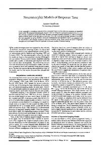
Fig. 1: Olfactory information processing2. Odorant molecules entering the nostrils bind to receptor neuron in the olfactory epithelium. Odor signals from the receptor neurons are then relayed to olfactory bulb where the bulk of signal processing takes place. Bulbar outputs are then passed onto olfactory cortex, where they are interpreted as different odors.
2
Adapted from: http://www.sfn.org/content/Publications/BrainBriefings/smell.html
I. Receptors
5
1 ORN
II. Olfactory Bulb
2
3
4
6
III. Olfactory Cortex
5
Fig. 2: Different anatomical stages and signal-processing primitives in the olfactory pathway (adapted from Mori et al. 1999): (1) population coding, (2) chemotopic convergence, (3) gain control, (4) contrast enhancement, (5) storage and association of odor memories and (6) bulbar modulation through cortical feedback. The first primitive is concerned with transduction of the chemical stimulus into an electrical signal. Odorants are volatile compounds with low molecular weight (30300 Dalton), typically organic, hydrophobic and polar (Schiffman and Pearce 2003).
6
Three notable theories have been proposed that relate molecular properties of an odorant with its overall quality: vibrational, steric, and odotope theories (Dyson 1938; Moncrieff 1949; Shepherd 1987). The vibrational theory first proposed by Dyson (1938) and later revisited by Wright (1982) and Turin (1996) (Lefingwell 2002), suggests that vibrations due to stretching and bending of odor molecules are the determinants of odor identity and quality. On the other hand, the steric theory initially put forth by Moncreiff (1949) and later extended by Amoore (1970) (Lefingwell 2002) proposes that odor quality is determined by the shape and size of the odorant molecules. More recently, the odotope or weak shape theory was proposed by Shepherd (1987). According to this theory, odor quality is determined by various molecular features of an odorant (commonly referred to as odotopes), such as carbon chain length or different functional groups. Though the precise relationship between the molecular properties and the odorant quality is still not known; much has been recently discovered about the olfactory transduction mechanism. Odorant molecules that enter the nostrils bind to olfactory receptor neurons, which belong to a family of G-protein coupled receptors (Axel 1991). As illustrated in Fig. 3, these receptors cross the cell membrane seven times (seventransmembrane) forming pockets where the odorants bind. The odorant-bound receptor triggers a cascade of molecular events that transform the chemical signal into a neural signal. A detailed illustration of this mechanism is shown in Fig. 4. First, tens of Gproteins are released by the activated receptor, which in turn activate the transducer Adenylyl cyclase (AC). Once activated the adenylyl cyclase converts the abundant Adenosine
TriPhosphate
(ATP)
intracellular
molecules
into
cyclic-3’,5’-
7
AdenosylMonoPhosphate (cAMP) secondary messengers.
The cAMP binds to the
cyclic nucleotide channel (CNG) and opens it to allow Na2+ and Ca2+ cations inside. This depolarizes the cell and, if the gates are open long enough, causes it to fire an action potential (Firestein 2001).
Outer Cell-membrane Inner Cell-membrane
Fig. 3:
G-protein coupled odorant receptors make seven loops through the cell
membrane, forming pockets for holding odor molecules. Each receptor type is specified by a particular sequence of a string of amino acids.
Rearranging the amino acid
sequence results in a different receptor type. Approximately 1,000 different receptors have been known to exist in the case of mammals. (reprinted from Mombaerts 2004; Laurent 2005).
8
A complete model of the transduction (Malaka 1995) is beyond the scope of this work; let it suffice that the spiking frequency of an ORN is a monotonically increasing function of the odorant concentration for a given receptor-odorant binding affinity. Each ORN responds to a range of odorants and each odorant is encoded by a large population of such cross-selective ORNs. To illustrate the combinatorial nature of the odor code available at the olfactory epithelium, Fig. 5 shows the response of sixty different ORNs to twenty odorants (Sicard and Holey 1982). Each receptor exhibits broad tuning and responds to a number of odorants.
Fig. 4: Olfactory signal transduction mechanism. Binding of an odorant molecule to a receptor triggers a cascade of molecular mechanisms, finally leading to depolarization of the neuron and generation of an action potential (reprinted from Firestein 2001).
9
Fig. 5: Combinatorial coding by ORNs. Columns indicate odors; rows indicate receptor cells identified by a serial number given in the leftmost column. ACE – acetophenone, ANI – anisole, BUT – n-butanol, CAM – DL-camphor, CDN – cyclodecanone, CIN – 1,8-cineole, CYM – p-cymene, DCI – D-critonellol, HEP– n-heptanol, ISO – isoamylacetate, IVA – isophenol, PHO – thiophenol, PYR – pyridine, THY – thymol, XOL – cyclohexanol, XON – cyclohexanone. The spot size is roughly proportional to spike frequency (spike/min). (Reprinted from Sicard and Holey 1982).
10
The next three signal-processing primitives take place at the olfactory bulb (OB). The second primitive involves massive convergence of ORN axons onto one or a few glomeruli (GL) [Mori et al. 1999; Laurent 1999], which are spherical structures of neuropil on which ORNs synapse mitral cells. Fig. 6 shows the convergence of ORNs expressing the same P2 receptor onto a single GL in the mouse OB [Bulfone et al. 1998]. This form of convergence serves two computational functions.
First, massive
summation of ORN inputs averages out uncorrelated noise, allowing the system to detect odorants below the detection threshold of individual ORNs. This is discussed later in section I.3.
Second, chemotopic organization leads to a more compact odorant
representation than that available at the epithelium, providing the means to decouple odor quality from odor intensity. This is the basis for the traditional view of GL as labeled lines (one GL: one odor) or, more recently, as odotope detectors (one GL: one molecular feature) [Mori et al. 1999]. The GL maps of four different odors: pentanoic acid, methyl pentanoate, pentanol, and pentanal, and a single analyte (methyl pentanoate) at different concentrations are shown in Fig. 7. These maps were obtained in rat olfactory bulb using optical imaging techniques involving 2-deoxyglucose uptakes. It can be seen that the identity of the odor is encoded by a unique spatial pattern across GLs, whereas the odor concentration is related to the intensity and spread of this pattern (Johnson and Leon 2000).
11
Fig. 6: Convergence of ORNs expressing P2 receptor onto a single GL in the mouse OB (Bulfone et al. 1998).
12
a) Glomerular maps across odors
pentanoic acid
methyl pentanoate
pentanol
pentanal
b) Glomerular maps across concentration (methyl pentanoate) Concentration
Fig. 7: Glomerular-layer activity patterns in rat olfactory bulb: identity is encoded by a unique spatial pattern across GLs (top row); concentration is related to the intensity and spread of this pattern (bottom row) (Johnson and Leon 2000). The initial glomerular image is further transformed in the olfactory bulb by means of two distinct lateral inhibitory circuits.
The first of these circuits (third
primitive in Fig. 2) takes place between proximal GLs through periglomerular (PG) cells.
As noted by Freeman (1999), the interaction through PG cells may serve as a
13
“volume control” mechanism, enabling the identification of odorants over several log units of concentration. Recently, local neurons in the moth antennal lobe (analogous to PG cells in the olfactory bulb of mammals) have been found to operate as multifunctional units, causing local inhibition at lower odor concentrations and global inhibition at higher concentrations (Christensen et al. 2001). This result is particularly interesting and will be discussed later in Chapter IV. The fourth primitive is represented by dendro-dendritic interactions between excitatory mitral/tufted (M/T) and inhibitory granule (GR) cells. These self and lateral inhibitory circuits form the negative feedback loops that are responsible for the observed oscillatory behavior in OB (Segev 1999). More importantly, local inhibition introduces time as an additional coding dimension by generating temporal patterning of the initial spatial code at the GL layer (Shepherd et al. 2003). The precise role of the granular lateral inhibition circuits is, however, under debate.
Two hypotheses have been
suggested for the role of these circuits. The first and more traditional view is that lateral inhibition sharpens the molecular tuning range of individual mitral cells with respect to that of their corresponding ORNs (Mori et al. 1999). This is illustrated in Fig. 8, where the GL unit (indicated by B) responds to a wide range of odorants (aldehydes with hydrocarbon chain length from five to nine), whereas the M cell receiving this input (indicated by D) exhibits a shaper tuning range (D responds to aldehydes with hydrocarbon chain length from six to eight) due to lateral inhibition from neighboring M cells through GR cells. Taken to the extreme, this function reduces to the Winner-TakeAll strategy of competitive learning. The second hypothesis for the role of lateral
14
inhibition is that it leads to a “global redistribution” of activity such that the bulb-wide representation of an odorant, rather than the individual tuning ranges, becomes specific and concise over time (Laurent 1999). Fig. 9 shows the odor trajectories formed by the spatio-temporal activity of projection neurons in the honeybee antennal lobe (analogous to M cells in mammalian OB); AL activity evolves over time, moving away and settling into odor specific regions. This neuro-dynamics view of lateral inhibition is thus heavily related to temporal coding. This temporal coding mechanism will be discussed further in Chapter V.
A ORN
3 4 5 6 7 8 9 10 11 n-CHO
B A
B
C GL
3 4 5 6 7 8 9 10 11 n-CHO
C
D
M/T
3 4 5 6 7 8 9 10 11 n-CHO
D GR
(+) (-) 3 4 5 6 7 8 9 10 11 n-CHO
Fig. 8: Sharpening of molecular tuning range through lateral inhibition. A, B, and C are GL units that respond to aldehydes with hydrocarbon chain length from three to eight, five to ten and seven to eleven, respectively. Mitral cell D, which receives input from B, exhibits a shaper tuning range than B and responds to aldehydes with hydrocarbon chain length from six to eight due to lateral inhibition from neighboring mitral cells (adapted from Yokoi et al. 1995).
15
Fig. 9: Odor trajectories formed by spatio-temporal activity in the honeybee AL. The spatio-temporal response of the twenty-one PNs was projected along their first three principal components for visualization purposes. The trajectories begin close to each other, and evolve over time to converge into odor specific attractors. (reprinted from Galan et al. 2003). The fifth primitive involves the formation of “odor objects” and their subsequent storage in the piriform cortex (PC). Pyramidal neurons (P), the principal cells in the PC, receive sparse, non-topographic, excitatory connections from M/T axons in the OB through the lateral olfactory tract (LOT). These projections are both convergent and divergent (many-to-many).
This suggests that P cells detect combinations of co-
occurring molecular features of the odorant, and therefore function as “coincidence
16
detectors” (Wilson and Stevenson
2003). The PC is also characterized by sparse,
distributed connections between P cells. These lateral connections have been shown to play an important role in storing odors with minimum interference and pattern completion of degraded stimuli (Wilson and Bower 1988).
Together, these two
anatomical features of the PC (many-to-many connection from OB and lateral association connections between P cells) form the basis for the synthetic processing of odors (Wilson and Stevenson 2003). The sixth primitive involves centrifugal connections from the cortex onto GR interneurons in the olfactory bulb.
Several computational functions have been
associated with these feedback connections, including odor segmentation and habituation (Li and Hertz 2000), hierarchical clustering (Ambrose-Ingerson et al. 1990), and chaotic bulbar dynamics (Yao and Freeman 1990). We have presented a review of our current understanding of information processing strategies in the biological olfactory system. Next, we present an overview of current sensing technologies and pattern recognition approaches in e-noses. I.2. The electronic nose An electronic nose is an instrument that combines an array of cross-selective chemical sensors and a pattern recognition engine to recognize odors (Persaud and Dodd 1982). The processing of multivariate sensor responses is usually performed by means of statistical pattern recognition (Gutierrez-Osuna 2002), as illustrated in Fig. 10 (Nagle et al. 1998).
17
Sensor array
Preprocessing
r r r u=v v ∆R
Dimensionality Reduction
Classification Regression Clustering
Validation
f2
R0
f1
Optimization feedback
Fig. 10: Building blocks of sensor-based machine olfaction architecture: (i) sensor array, (ii) signal preprocessing, (iii) dimensionality reduction, (iv) classification, and (v) validation (reprinted from Gutierrez-Osuna 2002). I.2.1. Review of sensor technologies A number of sensor technologies have been employed for the purpose of detecting and identifying chemicals, including metal-oxide (MOS) and conducting polymer (CP) chemoresistors, quartz microbalance (QMB) resonators, surface acoustic waves (SAW) devices, and optical-fiber based devices.
Fig. 11 provides an illustration of the
underlying principles used by these different types of sensors. MOS sensors detect odorants through changes in conductance of the sensing material due to oxidation/reduction reactions caused by the odorant (Nagle et al. 1998). In the case of CP sensors, the odorants interact with the polymer (usually polypyrole, polythiophene or polyaniline) by directly accepting ions from the polymer chain, interacting with the dopant ions (e.g., chloride ions) or diffusing into the polymer lattice causing it to swell (Nagle et al. 1998; Yinon 2003). These interactions change the conductivity of the material, which is read out as the sensor signal (Nagle et al. 1998).
18
(a)
(b)
(c)
(d)
Fig. 11: Chemical sensing technologies: (a) Metal-oxide sensors (MOS)/ Conducting Polymer (CP) chemoresistors; (b) Quartz crystal microbalance (QCM) resonators; (c) Surface Acoustic Waves (SAW) devices; (d) Optical fiber sensors (Nagle et al. 1998). QCM and SAW sensors employ a completely different sensing principle for detecting odorants compared to MOS and CP sensors. In the case of QCM, odorants adsorb to the surface of a piezoelectric quartz crystal, altering its mass and therefore shifting its resonant frequency (Nagle et al. 1998). On the other hand, in SAW sensors, an A.C voltage is applied to the input electrode, generating an acoustic wave that propagates through the surface of the piezoelectric material. Odorants adsorb to the
19
active material in the propagation path, which alters the surface characteristics and affects the velocity of the acoustic wave. The change in the velocity, measured by monitoring the phase shifts of the signal at the output electrode, becomes the sensor response (Nagle et al. 1998). In the case of optical fiber sensors, fluorescent dyes are immobilized in the polymer matrices placed on one end of the fibers. Exposure to odorants alters the microenvironmental polarity of the dyes in the polymer matrices. The dyes respond with a corresponding shift in their fluorescent spectrum, which becomes the sensor response (Dickinson et al. 1996). The reader is referred to (Nagle et al. 1998) for an introductory review of odor sensing technologies. The transduction principles for MOS sensor and optical fiber sensors, which are used in this dissertation, will be discussed in detail in Chapter II. I.2.2. Review of pattern recognition for chemical sensor arrays The multivariate sensor array response is then regarded as a fingerprint of the stimulus. These raw signals are first preprocessed to accomplish several functions, such as drift compensation, feature extraction and reduction of sample-to-sample variance (Nagle et al. 1998).
Preprocessing is followed by a dimensionality reduction stage.
Linear
techniques such as principal component analysis (PCA) and linear discriminant analysis (LDA), non-linear techniques such as Kohonen self-organizing maps (SOM) and several feature selection approaches have been widely used for this purpose (Nagle et al. 1998; Pearce 1997).
These lower-dimensional odor signals are then passed to a pattern
20
classification algorithm to predict the identity of the stimulus from among a finite set of previously learned classes. A number of pattern classifiers have been used with gas sensor arrays. Fig. 12 shows a summary of statistical methods that have been used for pattern analysis with gas sensor arrays. Readers are referred to (Schiffman and Pearce 2003; Gutierrez-Osuna 2002) for a thorough review of these methods. These statistical techniques have been used extensively for handling generic pattern recognition tasks such as dimensionality reduction, 1-of-m classification, and clustering (Pearce 1997; Gutierrez-Osuna 1998 and references therein). Problems unique to chemical sensors such as estimating chemical concentrations in a mixture (Ortega et al. 2000; Sundic et al. 2003), canceling background odors (Gutierrez-Osuna and Powar 2003), handling odor mixtures (Capone et al. 2001; Yamanaka 2004), drift compensation (Gutierrez-Osuna 2000; Holmberg and Arthursson 2002), event detection (Perera et al. 2003) and prediction of sensory scores (Gutierrez-Osuna 2002) have also been tackled using these methods. The last problem, that of predicting organoleptic properties of odorants from their response on a sensor array, is arguably the ultimate challenge of machine olfaction, but also the least successful to date.
21
MDS PCA Unsupervised
SOM ICA CA
Dimensionality Dimensionalityreduction reduction
LDA Supervised
PLS FSS PCR MLR
Regression
CCR MLP
Multivariate MultivariateAnalysis Analysis
Classifiers Classifiers
Neural Nets
RBF PNN K-NN
Others
SVM ART GA Fuzzy methods k-means
Clustering Clustering
HC SOM
Fig. 12: Statistical methods for multivariate pattern analysis techniques applied with gas sensor arrays (Schiffman and Pearce 2003; Gutierrez-Osuna 2000, 2002; DeCoste et al. 2001). MDS- Multi-dimensional scaling, PCA- Principal Component Analysis, SOMSelf-Organized Maps, ICA- Independent Component Analysis, CA- Cluster Analysis, LDA- Linear Discriminant Analysis, PLS- Partial Least Squares, FSS- Feature Selection Search, PCR- Principal Component Regression, MLR- Multi Linear Regression, CCRCanonical Correlation Regression, MLP- Multi-Layer Perceptron, RBF- Radial Basis Functions, PNN- Probabilistic Neural Network, k-NN- k-Nearest Neighbors, SVMSupport Vector Machines, ART- Adaptive Resonance Theory, GA- Genetic Algorithms, and HC- Hierarchical Clustering.
22
I.3. Neuromorphic processing for chemical sensor arrays Leveraging a growing body of knowledge from computational neuroscience (Davies and Eichenbaum 1991), neuromorphic models of the olfactory system have become a recent subject of attention for the purpose of processing data from chemical sensor arrays. Ratton et al. (1997) have employed the olfactory model of Ambros-Ingerson et al. (1990), which simulates the closed-loop interactions between the olfactory bulb and higher cortical areas. The model performs a hierarchical processing of an input stimulus into increasingly finer descriptions by repetitive projection of bulbar activity to (and feedback from) the olfactory cortex.
Ratton et al. (1997) have applied the model to
classify data from a micro-hotplate metal oxide sensor excited with a saw-tooth temperature profile. Sensor data was converted into a binary representation by means of thermometer and Gray coding, which was then used to simulate the spatial activity at the olfactory bulb.
Their results show that classical approaches (Gram-Schmidt
orthogonalization, fast Fourier transform and Haar wavelets) yield better classification performance. This result should come as no surprise given that the thermometer and Gray codes are unable to faithfully simulate the spatial activity at the olfactory bulb, where the most critical representation of an odor stimulus is formed. White et al.
(1998, 1999) have employed a spiking neuron model of the
peripheral olfactory system to process signals from fiber-optic sensor array. In their model, the response of each sensor is converted into a pattern of spikes across a population of ORNs, which then projects to a unique mitral cell.
Different odors
produce unique spatio-temporal activation patterns across mitral cells, which are then
23
discriminated with a delay line neural network (DLNN). Their OB-DLNN model is able to produce a decoupled odor code: odor quality being encoded by the spatial activity across units, and odor intensity by the response latency of the units. Pearce et al. (2001) have investigated the issue of concentration hyperacuity by means of massive convergence of ORNs onto GL. Modeling spike trains of individual ORNs as Poisson processes, the authors show that an enhancement in sensitivity of
n
can be achieved at the GL, where n is the number of convergent ORNs. Experimental results on an array of optical micro-beads are presented to validate the theoretical predictions. Otto et al. (2000) have employed the KIII model of Freeman et al. (1998) to process data from FT-IR spectra (Quarder et al. 2001; Claussnitzer et al. 2001) and chemical sensors (Otto et al. 2000). The KIII is a neurodynamics model that faithfully captures the spatio-temporal activity in the olfactory bulb, as observed in electroencephalogram (EEG) recordings. In (Quarder et al. 2001), the FT-IR spectrum of each analyte was decimated, Hadamard-transformed and normalized before being used as an input vector into the KIII model. The authors show that the principal components of the mitral cell state-space attractors can be used to discriminate different analytes. Their results, however, indicate that the KIII is unable to match the performance of a Regularized Discriminant Analysis classifier. Gill and Pearce (2003) have used an array of optical micro-bead sensors to investigate the issues of development, organization and maintenance of connections in the early olfactory pathway. Two populations of micro-bead sensors: active (exposed to
24
various odorants) and inactive (exposed only to air) were used to simulate the distribution of ORNs in the olfactory epithelium. Oja’s Hebbian learning rule was used to develop activity-dependent weights between the sensor (receptor) layer and the GL layer; a Mexican hat function was used to model the lateral interactions between GLs mediated by PG cells. Similar to experimental findings on mice (Zheng et al. 2000), their results show segregation of the active and inactive ORN populations into separate GLs suggesting the influence of odorant-evoked activity in the organization and maintenance of OB connections. Further their results suggest that the lateral interaction between GLs through PG cells play an important role in realizing the topological organization of the ORN projections. However, this predicted role of PG cells has not been confirmed through experimental studies. Gutierrez-Osuna et al. (2003a, 2003b) has investigated the use of habituation for processing odor mixtures with chemical sensor arrays. A statistical pattern recognition model was presented in (Gutierrez-Osuna and Powar 2003), where habituation is triggered by a global cortical feedback signal, in a manner akin to Li and Hertz (2000). A neuromorphic approach based on the KIII model was proposed in (Gutierrez-Osuna and Gutierrez-Galvez 2003), where habituation is simulated by local synaptic depression of mitral channels. Inspired by the role of GL as functional units (Pearce 1997), sensor array patterns are preprocessed with a family of odor selective discriminant functions before being fed to the KIII model. Their results showed that the KIII model is able to recover the majority of the errors, introduced in the sensor-array and discriminantfunction stages, by means of its Hebbian pattern-completion capabilities.
25
With the exception of prior work in our group, the use of neuromorphic models has focused on 1-of-m classification (Ratton et al. 1997; Otto et al. 2000; White et al. 1998) and sensitivity enhancement (Pearce et al. 2001). Problems of dimensionality reduction, gain control and intensity/quality coding have not been investigated using neuromorphic approaches.
In this dissertation, we address this issue and propose
neuromorphic solutions to these problems. I.4. Proposed work: Biologically-inspired computational models for machine olfaction Based on the computational view of the olfactory pathway presented in section I.1, this dissertation proposes a biologically-inspired architecture for the processing of gas sensor array signals.
Shown in Fig. 13, the architecture consists of six building blocks,
modeled after the six signal processing primitives identified in the olfactory pathway. First, a high dimensional odor signal is generated from the sensor arrays using a variety of methods that will be discussed in Chapter II. This high dimensional odor signal undergoes dimensionality reduction through chemotopic convergence, producing an odor image that decouples odor identity from intensity.
The odor images formed
through convergence are highly overlapping, and are subsequently processed by two lateral inhibitory circuits. The first circuit performs gain control, enabling identification of the odorant across a wide range of concentration. The second lateral inhibitory circuit enhances the initial contrast between odor images. The sharpened odor image is stored in a content addressable memory (CAM). Finally, interaction between the CAM and the
26
contrast enhancement circuits performs mixture segmentation and background suppression. In the following chapters we will propose computational models of these six signal-processing primitives, which are all novel to machine olfaction. We will validate these models on experimental datasets generated using sensor arrays employing MOS and optical fiber sensors and Infrared absorption spectroscopy. Olfactory Epithelium Sensor array
Olfactory Bulb
High-dimensional Dimensionality Reduction odor signal c2
VH
RH
Gain control
Olfactory Cortex Contrast Enhancement
Content Addressable Memory
r r r u=v v
RS
c1
Segmentation/ background suppression
Fig. 13: Building blocks for biologically-inspired pattern recognition in sensor-based machine olfaction. The six stages correspond to the six signal processing primitives identified in the olfactory pathway (refer to Fig. 2). I.5. Contributions of this work The principal contributions of this dissertation research can be summarized as follows: (1) We have developed computational models of key signal processing primitives in the olfactory system, and integrated them in a neuromorphic architecture suitable for machine olfaction with gas sensor arrays.
27
(2) We have characterized the proposed models and validated them on experimental datasets from temperature-modulated metal oxide chemoresistors and a large population of optical microbead sensors. (3) We have conducted a preliminary investigation to examine the relationships between molecular features of odorants detected by their infrared absorption spectra, and their olfactory bulb images, and their overall smell descriptors. I.6. Organization of this document The rest of this dissertation is organized as follows: Chapter II describes three separate methods that can be used to generate a high-dimensional, combinatorial input signal from gas sensor arrays. Chapter III presents a computational model of receptor neuron convergence that generates compact odorant representations similar to those observed in the olfactory bulb. Chapter IV presents a model of shunting lateral inhibition that removes concentration effects from the multivariate response of a gas sensor array. Chapter V presents an additive model of lateral inhibition with center-surround connections that improves contrast between odor images formed after chemotopic convergence. Chapter VI presents a model of bulbar-cortical interactions capable of achieving background suppression and mixture segmentation. Chapter VII integrates the six primitives to create a unified neuromorphic signal processing architecture for machine olfaction. Chapter VIII presents a summary of results and identifies directions for future research. Supplementary materials are provided as three separate appendices. Appendix A includes a table with the range of IR absorption spectra for different functional groups;
28
this reference material is useful for illustrating the IR principle in Chapter II. Appendix B presents a computational model for olfactory receptors that can be used to generate high-dimensional signals from the low-dimensional feature spaces typically obtained with e-nose instruments. Appendix C presents a spiking model of the OB; this model shows that the proposed primitives are not tied to any particular neural network model (e.g., spiking vs. rate model).
29
CHAPTER II HIGH-DIMENSIONAL ODOR CODING WITH PSEUDO-SENSORS
The first stage in the olfactory pathway consists of a large array (~10-100 million) of sensory neurons, each of which selectively expresses one or a few genes from a large (~1,000) family of receptor proteins (Buck and Axel, 1991). Each receptor is capable of detecting multiple odorants, and each odorant can be detected by multiple receptors, leading to a massively combinatorial olfactory code at the receptor level. It has been shown (Alkasab et al. 2002; Zhang and Sejnowski 1999) that this broad tuning of receptors may be an advantageous strategy for sensory systems dealing with a very large detection space.
This is certainly the case for the human olfactory system, which has
been estimated to discriminate up to 10,000 different odorants (Schiffman and Pearce, 2003). Further, the massively redundant representation improves signal-to-noise ratio, providing increased sensitivity in the subsequent processing layers (Pearce et al. 2002). Unlike the biological olfactory system, the artificial system uses very few sensors, commonly one replica of up to 32-64 different sensor types. This fundamental mismatch between the two systems in their input dimensionality must be overcome in order to be able to exploit the processing strategies employed by the biological olfactory system. In order to generate a combinatorial and high dimensional odor representation from chemical sensor arrays, similar to that available in the olfactory epithelium, we will adopt the following three mechanisms:
30
•
Temperature modulation in metal-oxide sensors,
•
Sensing with a large population of optical microbead arrays, and
•
Infrared absorption spectroscopy.
The objective of this chapter is to present and analyze each one of these dimensionality expansion techniques. II.1. MOS sensor array The first method to simulate a large population of cross-selective sensors involves temperature modulation of metal oxide (MOS) chemoresistors. The various components of a MOS sensor are shown in Fig. 14. The sensing material is a metal oxide (tin, zinc, titanium, or iridium) coated with a noble metal catalyst (palladium or platinum) (Nagle et al. 1998). The active material is placed on a substrate made of silicon, glass or plastic, and heated by applying a voltage to a resistive heating built into the device. When the heated
active
material
comes
in
contact
with
the
odorant,
it
undergoes
reduction/oxidation chemical reaction depending on the nature of the environment. In an oxidizing atmosphere, oxygen ions resulting from the decomposition of oxygen molecules in the ambient, or other electron acceptors adsorb to the surface of the material and trap free electrons from the conduction band of the semiconductor as shown in Fig. 15(a). This results in a decrease in the conductance of the sensing material. In a reducing atmosphere, on the other hand, the adsorbed oxygen atoms react with the reducing ambient molecules, releasing the trapped electrons to the sensing material as shown in Fig. 15(b). This results in an increase in the conductance of the sensing
31
material. The change in conductivity of the active material is measured by observing the change in resistance across the electrode pair below the active material.
Fig. 14: General structure of a metal-oxide semiconductor chemoresistor (Nagle et al. 1998).
32
(a) O2
O2 O2 + e- Æ O-2 ½O2 + e- Æ O½O2 + 2e- Æ O2-
SnO2 grains
O2
O-2 O-2 O-2 O-2 e O e e 2 O 2 - e- e- e e eee- O 2 O 2 - - - e- Oe 2 e e e O-2 e- e O O 2 2 O-2 eVs in air
electrons
(b) CO
O2
O2
CO
O2
eeee- e- eO e 2 e e e- e e eeee- e - e- ee e e e e- e- e eee
O-2 + CO Æ CO2 + eO- + CO Æ CO2 + eO2- + CO Æ CO2 + 2e-
eVs in the presence of reducing gas
Fig. 15: (a) Atmospheric oxygen adsorbed on the surface of the metal oxide trap free electrons from the conduction band of the semiconductor. This causes a potential barrier (eVs), which prevents electrons from moving freely, reducing the sensor conductance. (b) In the presence of reducing gas, the adsorbed oxygen atoms react with the reducing ambient molecules, releasing the trapped electrons.
The potential barrier (eVs)
decreases allowing electrons to move freely increasing the sensor conductance. (adapted from Figaro 1996).
33
II.1.1. Temperature modulation In the case of MOS materials, the relative selectivity to different volatiles is known to be a function of the operating temperature at the surface of the material (Lee and Reddy 1999).
This operating temperature is typically maintained at a constant set-point
(specified by the manufacturer). This form of excitation is commonly referred to as isothermal operation. However, due to the temperature-selectivity dependence of MOS devices, more information can be extracted from the sensor by simply modulating the heater voltage during exposure to a volatile and capturing the dynamic response of the sensor at each heater voltage. The process is illustrated in Fig. 16. A sinusoidal voltage is applied to the sensor’s heater, and the dynamic response of the sensing element is recorded simultaneously. If the heater voltage is modulated slowly enough relative to the thermal time constants of the device, the response of the sensor at each heater voltage can be considered a separate “pseudo-sensor”, and used to simulate a large population of ORNs.
34
VH
VH
RH
RS VS
time 1/RS
RL
VOUT pseudo sensor i
pseudo sensor j
time
Fig. 16: Temperature modulation for metal-oxide sensors. A sinusoidal voltage VH is applied to a resistive heather RH, and the sensor resistance RS is measured as a voltage drop across a load resistor RL on a half-bridge. Due to the temperature-selectivity dependence, the response of a sensor at a particular temperature can be treated as a separate “pseudo-sensor,” and used to simulate a large population of ORNs. II.1.2. Selectivity data set (Powar 2002) In order to generate a high-dimensional sensor response to overcome the dimensionality mismatch between the artificial olfactory system and its biological counterpart and validate the models presented in the following chapters, we perform temperature modulation of two Figaro MOS sensors (TGS 2600, TGS 2620) (Figaro 1996). A sinusoidal heater voltage (1-7 V range) with a 150 seconds time period, shown in Fig. 17, is used for this purpose. The sensor response is sampled at 10 Hz, leading to a population of 1500 pseudo-sensors from each sensor. The sensor array is exposed to the static headspace of mixtures from three analytes: acetone (A), isopropyl alcohol (B) and
35
ammonia (C), at three dilution levels in distilled water (the neutral). The lowest dilution of the analytes is 0.3 v/v% for acetone, 1.0 v/v% for isopropyl alcohol and 33 v/v% for ammonia. These baseline dilutions were chosen so that the average isothermal response (i.e., a constant heater voltage of 5V) across the two sensors was similar for the three analytes, thus ensuring that they could not be trivially discriminated (Gutierrez-Osuna and Raman 2004). Two serial dilutions by a factor of 1/3 were also acquired, resulting in 21 samples per day (4 mixtures × 3 concentrations). The process was repeated on three separate days, for a total of 63 samples. The temperature-modulated response of the two sensors to the three concentrations of the single analytes is shown in Fig. 18. Each analyte leads to a unique pattern, defined by the amplitude and location of a maximum in conductance. Two maxima are easily resolved in the case of isopropyl alcohol. 7
Voltage
6
5
4
3
2
1
20
40
60
80
100
120
140
Time (in sec)
Fig. 17: Sinusoidal heater voltage profile used for modulating the operating temperature of the MOS sensors.
36
Sensor 1
Sensor 2
1
Sensor conductance (normalized)
0.9
Isopropyl Alcohol
Ammonia
0.8 0.7 0.6 0.5 0.4 0.3
Acetone
0.2 0.1 0
500
1000
1500
2000
2500
3000
Pseudo-sensors Fig. 18: Temperature-modulated response of two MOS sensors (concatenated) to acetone (odor A), isopropyl alcohol (odor B) and ammonia (odor C) at three concentrations. Three replicates per analyte and concentration are shown in the figure to illustrate the repeatability of the patterns. The temperature-modulated response of one MOS sensors to binary and ternary mixtures at the highest concentration is shown in Fig. 19. It can be seen that the sensor responses show some degree of additivity with respect to the single analyte responses, particularly in the case of binary mixtures. We will show later that this type of additivity in the sensor response is necessary for segmenting mixtures into their constituents.
37
Sensor Conductance
1.2
(1)
Mixture (AB)
Acetone (A)
1
Iso-propyl alcohol (B) 0.8 0.6 0.4 0.2
200
400
600
800
1000
1200
1400
Pseudo-sensors
Sensor Conductance
1.2
Acetone (A)
(2)
Mixture (AC)
1
Ammonia (C)
0.8 0.6 0.4 0.2
200
400
600
800
1000
1200
1400
Pseudo-sensors
Fig. 19: Temperature-modulated response of a TGS 2620 MOS sensor to three pure analytes and their binary mixtures: (1) acetone (A), isopropyl alcohol (B) and their binary mixture (AB); (2) acetone (A), ammonia (C) and their binary mixture (AC); (3) isopropyl alcohol (B), ammonia (C) and their binary mixture (BC); (4)acetone (A), isopropyl alcohol (B), ammonia (C) and their ternary mixture (ABC).
38
1
Sensor Conductance
0.9 0.8
(3) Iso-propyl alcohol (B)
0.7
Mixture (BC)
Ammonia (C)
0.6 0.5 0.4 0.3 0.2 0.1 200
400
600
800
1000
1200
1400
Pseudo-sensors
Sensor Conductance
1.2 1 0.8
Acetone (A)
(4) Iso-propyl alcohol (B)
Mixture (ABC)
Ammonia (C)
0.6 0.4 0.2
200
400
600
800
1000
Pseudo-sensors
(Fig. 19: continued)
1200
1400
39
II.2. Optical microbead array Walt and colleagues at Tufts University have proposed a novel method for chemical sensing based on optical microbead sensors. The microbead arrays typically include hundreds of broadly-tuned bead sensors, each belonging to a discrete class, randomly dispersed across the tip of an optical fiber (Dickinson et al. 1999).
The high-
dimensional, combinatorial response generate by the microbead arrays to odorants makes them an attractive alternative for use with neuromorphic models. II.2.1. Microbead transduction principle The basic transduction mechanism of microarray bead sensor arrays is as follows. Each microbead is coated with a polymer matrix onto which a salvotochromic dye (e.g. Nile red) is immobilized. The microbead is then placed on the distal end of an individual optical fibers, as shown in Fig. 20(inset A). The salvotochromic dyes change their color based on the polarity of the microenvironment, i.e. polymer surface polarity or odor exposure. Immobilizing these salvotochromic dyes in polymer matrices that vary in polarity, hydrophobicity, porosity, elasticity, and swelling tendency, creates unique sensing regions that interact differently with odor molecules, giving unique response to various odors (Dickinson et al. 1996). Fig. 20 shows the basic odor sensing process using the microbead sensor arrays. Odor vapor diffuses into the polymer coated on the distal end of the fiber and modifies the microenvironment polarity.
This causes the dyes to change their fluorescence
intensity, which is captured with a CCD camera and plotted over time.
40
t1
t2
t3
(inset B)
(inset A)
Fig. 20: Odor sensing using microbead arrays: Odor vapor is delivered to the distal end of the fiber. Exposure to odor vapor induces a change in fluorescence that is recorded and plotted versus time. (inset A) microspheres coated with a polymer matrix, onto which a salvotochromic dye (e.g. Nile red) is immobilized, randomly fill the distal end of the fiber. (inset B) distal end of the optical fiber from which the response is read (adapted from Dickinson et al. 1996).
41
II.2.2. Illumina data set We will use a database from Illumina. Inc3, comprising of transient responses of 586 microbead sensors to five analytes: Acetone (A), Ethyl Alcohol (EA), Ethyl hydroxide (EtOH), Methyl hydoxide (MeOH), and Toulene. Fig. 21 shows the transient response of 100 microbead sensors to acetone. The odorant was introduced at t=14 sec and removed at t=35 sec.
The response of each sensor to the odorant is obtained by
computing the difference between its steady state response (t=34 s) and baseline value (t=13 s).
3
Data from Illumina microbead arrays, which are not commercially available, will be obtained through an
existing collaboration between Illumina and our research group.
42
Odor introduced
Odor removed
4500 4000
Sensor response
3500 3000 2500 2000 1500 1000 500 0
0
10
20
30
40
50
60
70
80
90
Time
Fig. 21: Response of 100 microbead sensors to acetone (courtesy of Illumina, Inc.). The odor, acetone in this case, is introduced at t=14sec and removed at t=35 sec. II.3. Infrared spectroscopy The third approach that will be used in this dissertation to generate a high-dimensional response involves infrared absorption spectroscopy. Though very little is known about the molecular determinants of an odorant, it is widely believed that each GL unit (to which similar ORNs converge) acts like a “molecular feature detector” that identifies a particular molecular property, such as type and position of a functional group (Mori et
43
al. 1999). In the realm of instrumental data, infrared (IR) absorption spectroscopy is the closest match to this form of molecular detection. II.3.1. IR principle IR spectroscopy is based on the fact that different inter-atomic bonds in a molecule absorb IR radiation at unique wavelengths in the mid-IR range (4000-0 cm-1). The absorption spectrum can be divided into two distinct regions: the so-called “functionalgroup” region (4000-1500 cm-1) and the “fingerprint” region (4) are primarily driven by inputs and hence show high stability (converge to a fixed-point attractor) and less variance. For large receptive fields (r≤4), the net value of the lateral connections becomes excitatory, and the system fails to converge into fixed-point attractors. Hence we will not consider them for determining the optimal parameter value for this odor database. Fig. 41(a,b) shows the separability between various odors (Jodor) and across different concentrations within each odor (Jconc ) as a function of the receptive field width (r). From these results, it is clear that that the separability between pairs of odors increases as the width of the receptive field increases, whereas maximum concentration separability is achieved with small receptive fields. The maximum of the objective function Jbalance, which combines concentration-invariant separability and concentration separability, occurs at r=5, as shown in Fig. 41(c). This receptive field width will be used to quantify the benefits of the proposed model.
87
3
(a )
Jodor
2 .5 2 1 .5 1 0 .5
20
12
8
6
5
6
5
r 2 .6
(b )
Jconc
2 .1 1 .6 1 .1 0 .6
20
12
8
r 4 .5
(c )
Jbalance
4 3 .5 3 2 .5 2
20
12
8
6
5
r
Fig. 41: Discriminatory information of GL patterns as a function of receptive field width: (a) separability between odors Jodor (b) separability between concentrations within an odor Jconc, and (c) separability across odors and across concentrations (Selectivity dataset).
88
The steady-state spatial patterns for various receptive field widths (r>4) are shown in Fig. 42. Global connections lead to sparse representation (fewer active mitral cells) since highly active GL regions are able to suppress activity in other regions in the lattice with weak activity. This causes reduction in the overlap across patterns and improves odor separability.
r=20
r=12
r=8
r=6
r=5
on-off surround
Odor A
Odor B
Odor C local
global
Fig. 42: Characteristics of the spatial odor code for various receptive-field widths of center on-off surround lateral connections. Global connections result in more sparse patterns that provide better odor separability.
89
V.2.2. Spatial patterning of MOS sensor responses
In this section we qualitatively analyze the improvements in pattern separability that result from the center on-off surround connections (r=5). Fig. 43 (top row of each block) shows the spatial pattern that result from sensory convergence at the input of the OB. As a result of the chemotopic mapping, each odor generates a unique spatial pattern across units in the SOM. However, these spatial patterns are highly overlapping due to the collinearity of the sensors. Fig. 43 (bottom row of each block) shows the resulting spatial activities following stabilization of the center-surround lateral interactions in equation (5.1). Odor A leads to heavy activation on two highly-localized regions (spatial code: 13).
Odor B produces similar activation in regions 1 and 3, but also high
activation in region 4 (spatial code: 134). This unique region 4 corresponds to pseudosensors in the smaller peak that occurs for odor B alone (refer Fig. 18). Odor C produces heavy activation of regions 1, 2 and 5 (spatial code: 125). It is important to note that the location of these activation regions is concentration-invariant, but their amplitude and spread increases with concentration, in consistency with recent finding in neurobiology (Friedrich and Korsching 1997).
90
1 ACETONE
3
ISOPROPYL ALCOHOL
1
3 4
Center Surround
SOM
Center Surround
SOM
Center Surround
SOM
Higher Higher concentrations Concentrations
1 AMMONIA
2
5
Fig. 43: Spatial maps generated from temperature modulated MOS sensor response at the input (top row of each block) and output (bottom row of each block) of the olfactorybulb network. Three blocks are shown corresponding to three odors: acetone (first block), isopropyl alcohol (second block) and ammonia (third block). Five sparse coding regions that emerge as a result of the lateral interactions are shown on the right.
91
V.2.3. Temporal evolution of the odor trajectories
The spatial patterns in Fig. 43 only describe the information content in the steady-state response of the model. To analyze the temporal trajectory of each dynamic attractor, the 400-dimensional (20x20) space was projected onto the first three principal components of the data, which are shown in Fig. 44. Trajectories for each odor and concentration originate at nearby locations in state space, which correspond to the highly overlapping spatial patterns at the input of OB, shown in Fig. 43 (top row). As a result of center onoff-surround lateral connections, the activity for each odor slowly moves away from the initial location and settle into odor-specific fixed-point attractors, which correspond to the localized spatial patterns in Fig. 43 (middle row). Visual inspection of the steady-state response in Fig. 43 and the transient trajectories in Fig. 44 clearly shows that the lateral inhibitory network is able to significantly increase the contrast between different odors. Parallels between this odor code and recent findings in neurobiology are discussed in section V.2.4. separability of these patterns is analyzed systematically in section V.2.5.
The
92
Trajectories originating close to each other
Fig. 44: Evolution of OB activity along the first three principal components of the data. Nine trajectories are shown, one per odor and concentration in the data. The initial points in the trajectories are the spatial maps at the input of the OB network. Odor separability is improved as a result of lateral inhibition. V.2.4. Discussion: Temporal coding in the biological olfactory system and our model
A recent study of spatio-temporal activity of projection neurons (PN) in the honeybee antennal lobe (analogous to M cells in mammalian OB) by Galan et al. (2003), reveals evolution and convergence of the network activity into odor-specific attractors. Fig. 45(a) shows the projection of the spatio-temporal response of the twenty-one PNs along their first three principal components. These trajectories begin close to each other, and evolve over time to converge into odor specific regions. These experimental results are consistent with the attractor patterns emerging from our model. Furthermore, in-vivo
93
experiments conducted by Stopfer et al. (2003), to study odor identity and intensity coding in the locusts show hierarchical groupings of spatio-temporal PN activity according to odor identity, followed by odor intensity.
Fig. 45(b) illustrates this
grouping in the activity of fourteen PNs when exposed to three odors at five concentrations. Again, these results closely resemble the grouping of attractors in our model, shown in Fig. 44. (b)
(a)
octanol
hexanol
nonanol
isoamylacetate
Fig. 45: (a) Odor trajectories formed by spatio-temporal activity in the honeybee AL (adapted from Galan et al. 2003). (b) Identity and intensity clustering of spatio-temporal activity in the locust AL (adapted from Stopfer et al. 2003); arrows indicate the direction of increasing concentration.
94
V.2.5. Temporal evolution of pattern separability
To illustrate the benefits of the proposed model, we compare the resulting patternseparability against that which is available (1) from raw sensor data, (2) following chemotopic convergence, (3) at the output of the OB network without lateral connections, and (4) at the output of the OB network with random lateral connections. Fig. 46(a-c) shows the temporal evolution of the separability measures Jodor, Jconc and Jbalance for each of these cases.
Fig. 46(a) indicates that chemotopic convergence
provides better concentration-invariant separability than raw temperature-modulated signals. On the other hand, Fig. 46(b) shows that random connections can in some cases provide better concentration discrimination than center-surround connections, but have significantly lower concentration-invariant separability as shown in Fig. 46(a). Overall, center on-off surround lateral connections (three repetitions are shown using different initial weights) provides maximum contrast between odor patterns amongst the compared schemes, and yields maximum value for the joint objective function Jbalance as shown in Fig. 46(c).
95
3
(a) 2.5 Center-Surround (3 curves)
Jodor
2
Input of OB
1.5 1 Random (3 curves)
0.5
Raw data, No lateral connections 0 0
100
200
300
400
500
Time (ms)
Fig. 46: Comparison of the additive model of OB lateral inhibition with center-surround lateral connections (three repetitions are shown) against (1) raw temperature-modulated data, (2) following chemotopic convergence, (3) at the output of OB with no lateral connections, and (4) at the output of OB with random lateral connections (three repetitions). (a) Concentration-invariant recognition measure Jodor, (b) concentration discrimination measure Jconc, and (c) balanced measure Jbalance.
96
3
(b)
Center-Surround (3 curves)
Input of OB
2.5
Random (3 curves)
Jconc
2 1.5 1 Raw data, No lateral connections
0.5 0 0
100
200
300
400
500
Time (ms) 5
(c)
Center-Surround (3 curves)
Jbalance
4.5 4
Input of OB
3.5 3
Random (3 curves)
2.5 Raw data, No lateral connections 2 0
100
200
300
400
500
Time (ms)
(Fig. 46: continued) V.3. Validation on the Illumina dataset
In this section, we characterize the center-surround lateral inhibition model on the Illumina dataset and present the improvements in odor separability achieved on this
97
dataset. The microbead array response is chemotopically projected onto a GL layer with 400 nodes, arranged as a 20x20 SOM lattice. The outputs of the convergence model are then used as the input for the neurodynamic OB model. The parameter a1 and a2 of the non-linear activation function are set to 0.0589 and 49.9999 respectively to match the dynamic range of the input signal from microbead arrays.
The appropriate lateral
inhibition spread (parameter r) is determined experimentally in a manner similar to the previous study on the Selectivity dataset. Results are shown in Fig. 47; separability between pairs of odors increases with the receptive field width till r=5. For receptive field width greater than r=5, small variations in the inputs are amplified considerably increasing the within-class scatter. 9 8
Jodor
7 6 5 4 3 2
20
12
8
6
5
4.5
4
r Fig. 47: Discriminatory information of GL patterns as a function of receptive field width (r).
Since the dataset contains the response of the optical microbeads to a single
concentration of five odors, the optimum center-surround width (r) can only be selected based on odor separability (Jodor).
98
V.3.1. Spatial patterning of microbead array responses
In this section, we qualitatively analyze the improvements in pattern separability that result from the center on-off surround connections (r=5). Fig. 48 (top row) shows the spatial patterns that result from sensory convergence at the input of the OB to five odors: (i) acetone (ACE), (ii) ehtyl alcohol (EA), (iii) ethyl hydroxide (Et-OH), (iv) methyl hydroxide (Me-OH) and (v) toluene (TOL). Each odor generates a unique spatial pattern across SOM units. Fig. 48 (middle row) shows the resulting spatial activities following stabilization of the center-surround lateral interactions. ACE leads to heavy activation on four highly-localized regions (spatial code: 123’4). EA and Et-OH produce similar activation as ACE in regions 2 and 4, but produce slightly different activation in regions 1 and 3 (spatial code: EA - 1’234; Et-OH - 1’234). Me-OH produces heavy activation of region 3 alone (spatial code: 3). TOL produces heavy activation of region 1, 2 and 4 (spatial code: 124). The spatial patterns after center-surround interactions are sparser than the chemotopic odor maps and provide better odor separability.
99
ETHYL METHYL TOLUENE HYDROXIDE HYDROXIDE
EA
Center Surround
SOM
ACETONE
1 4
2 3’
1’ 4
2 3
1’ 4
1
2 3
3
2
4
Fig. 48: Spatial maps at the input (top row) and output (middle row) of the OB network for the Illumina dataset. The bottom row shows the four sparse coding regions that emerge as a result of the lateral interactions. V.3.2. Temporal patterning
To study the temporal odor code, the 400-dimensional (20x20) OB model response is projected onto the first three principal components of the data, as shown in Fig. 49. Trajectories for each odor sample originate at nearby locations in state space. As a result of center on-off-surround lateral connections, the activity for each odor slowly moves away from the initial location and settles into odor-specific fixed-point attractors. The repeatability of the odor trajectories is illustrated by visualizing all twenty-five trajectories (five samples per odor) in the dataset. These results are qualitatively similar to those obtained on the Selectivity dataset (Fig. 44).
100
2 1.5
PC3
1 0.5
MeOH
Toluene
EA
0
EtOH -0.5 0
-2
-4
0 2
Acetone -6
-8
PC1
4 -10
6
PC2
Fig. 49: Evolution of OB activity for the Illumina dataset along the first three principal components. Twenty-five trajectories are shown, one per odor sample in the dataset. The initial points in the trajectories are the spatial maps at the input of the OB network, shown in Fig. 48 (top row).
Odor separability is improved as a result of lateral
inhibition. V.3.3. Temporal evolution of pattern separability
To illustrate the benefits of the proposed model, we compare the resulting patternseparability against that which is available (1) from raw sensor data, (2) following chemotopic convergence, (3) at the output of the OB network without lateral connections, and (4) at the output of the OB network with random lateral connections. Fig. 50 shows the temporal evolution of the odor separability for each of these cases. Similar to the results observed in the Selectivity dataset, center on-off surround lateral
101
connection provides maximum contrast between odor patterns amongst the compared schemes. 250
Center-Surround (3 curves)
Jodor
200
150
100
Input of OB, No lateral connections Raw data
50
Random (3 curves) 0
0
100
200
300
400
500
Time (ms)
Fig. 50: Comparison of the OB network with center-surround lateral connections (three repetitions are shown) against (1) raw temperature-modulated data, (2) following chemotopic convergence, (3) at the output of OB with no lateral connections, and (4) at the output of OB with random lateral connections (three repetitions). V.4. Summary
In this chapter, we have presented an additive model of lateral inhibition with center onoff surround receptive fields to model the circuits at the output of the bulb. This network is able to significantly reduce the overlap between the spatial odor patterns, and produces a sparser representation on a few selected mitral cells.
The spatial and
temporal odor code resulting from the center-surround interactions are consistent with
102
recent results from neurobiology.
The next stage of processing involves synthetic
processing of the odor signals in the cortex, and modulatory feedback to the bulb.
103
CHAPTER VI MIXTURE SEGMENTATION AND BACKGROUND SUPPRESSION THROUGH BULB-CORTEX INTERACTION
The last two olfactory primitives are concerned with the recognition of odorants against complex backgrounds, and the identification of the constituents in an odor mixture. Several studies have suggested that cortical feedback to the bulb may play an essential role in achieving these computational functions. Ambrose-Ingerson et al. (1990) have modeled the cortical feedback connections to account for hierarchical recognition of odors by humans. In this model, cues common to a subset of odorants are recognized before those that are odorant-specific. Li and Hertz (2000) have shown that centrifugal connections may cause odor-specific adaptation, leading to segmentation of odor mixtures. Grossberg (1976) has proposed that cortical connections to the bulb may selectively filter the bulb input and cause resonance between the two regions. Finally, Yao and Freeman (1990) have implicated these feedback connections with chaotic dynamics in the bulb. In this chapter, we will present a model of olfactory bulb–cortex interaction, and show that two different computational functions can be achieved (mixture segmentation, weaker odor/background suppression) depending upon the learning rule used to establish the cortical feedback connections to the bulb: antiHebbian or Hebbian, respectively. We validate these computational models to handle odor mixture signals on simulated odor patterns.
104
VI.1. Model of bulb-cortex interaction
The olfactory bulb sends non-topographic and many-to-many projections to the olfactory cortex. These convergent and divergent (many-to-many) projections suggest that cortical neurons detect combinations of co-occurring molecular features of the odorant, and therefore function as “coincidence detectors” (Wilson and Stevenson 2003). Fig. 51 illustrates the synthetic processing of odor signals through coincidence detection mechanism in the cortex. Since the number of possible combinations to be detected is extremely large, Laurent (1999) has suggested that these cortical cells perform a random sampling of this space. In our model with only few neurons, we simplify these circuits, and manually label the cortical cells to detect combinations of features for the odors in our datasets. Apart from these forward connections, the cortex is characterized by excitatory and inhibitory lateral connections that are known to play an important role in the storage of odors with minimum interference and pattern completion of degraded stimuli (Wilson and Bower 1988). Together, these two architectural features of the piriform cortex (many-to-many connection from OB, and lateral association connections between cortical cells) form the basis for the synthetic processing of odors (Wilson and Stevenson 2003).
105
Fig. 51: Synthetic processing by the cortical neurons through coincidence detection mechanism. (a) In response to a new odor the cortical neurons detect a particular combination of co-occurring molecular features identified by the mitral cells.
(b)
Adaptation of the afferent and association connections through learning enables the cortical neurons respond to odors as a whole when presented subsequently (reprinted from Wilson and Stevenson 2003). We model these olfactory circuits using an additive model, similar to the olfactory bulb model presented in Chapter V, as follows:
(
)
(
M dyiO (t ) yiO (t ) P =− + ∑ AC kiϕ y kO (t ) + ∑ FF jiϕ v Oj (t ) dt λi k =1 j =1
)
(6.1)
k ≠i
where yj is the activity of cortical pyramidal neuron i, λi is the time constant of the neuron, ACki is the synaptic weight between neurons k and i obtained through Hebbian learning, P is the number of neurons, FF is the feedforward connectivity matrix established through Hebbian learning, and vj is the activity of bulb neuron j.
106
Feedforward connections FF from bulb to cortex are established through a simple Hebbian learning rule as follows: FF = δ (VY T )
( Hebbian)
(6.2)
where Y is the matrix of cortical neuron outputs to different pure odors (row vectors manually labeled to recognized different odors), V is the matrix of bulb neuron outputs to pure odors (row vectors), and δ is a scaling parameter. Associational connections AC within cortex are established through a Hebbian update rule proposed in (Gutierrez-Galvez and Gutierrez-Osuna 2005) as follows: N
N
N
AC = α ⋅ ∑ Y O1 ⋅ (Y O1 ) T − β ⋅ ∑ ∑ Y O1 ⋅ (Y O2 ) T O1 =1
O1 =1 O2 =1 O2 ≠ O1
(6.3)
where Y O1 is the cortical response for odor O1, α and β are scaling parameters, which provide a necessary tradeoff between the first correlation term and the second decorrelation term. This form of update has been shown to enhance the contrast between input patterns (Gutierrez-Galvez and Gutierrez-Osuna 2005). In this case, this update rule results in associational connections such that neurons that code for at least one common odor have purely excitatory connections between them, and neurons that encode for different odors (no common odor) have purely inhibitory connections between them. Excitatory lateral connections perform pattern-completion of degraded inputs from the bulb (Wilson and Bower 1988), whereas the inhibitory connections introduce winner-take-all competition among cortical neurons (Xie et al. 2001). The last component of the model involves feedback connections from the cortex to the bulb. The cortical feedback is integrated to the OB model as follows:
107
dv Oj (t ) dt
=−
v Oj (t )
τj
(
)
(
P M O + ∑ Lkjϕ vkO (t ) + I O j + ∑ FBij ϕ yi (t ) k =1
i =1
)
(6.4)
where vj is the activity of bulb neuron j, τj is the time constant that captures the dynamics of the neuron, Lkj is the synaptic weight between neurons k and j, M is the number of neurons, Ij is the external input from the olfactory epithelium, FB is the feedback connectivity matrix, and yi is the activity of cortical neuron i. To model these feedback connections (FB) in equation (6.4), we use either antiHebbian or Hebbian rule as follows: FB = γ (−YV T )
(anti − Hebbian)
FB = γ (YV T )
( Hebbian)
(6.5)
where Y is the matrix of cortical neuron outputs to different pure odors (organized as row vectors), V is the matrix of bulb neuron outputs to pure odors (row vectors), and γ is a scaling parameter. In the case of anti-Hebbian learning, all connections are initialized to 0. The anti-Hebbian update forms feedback connections between the cortical and the bulb neurons that respond to at least one common odor. The resulting feedback from cortex inhibits bulbar neurons responsible for the cortical response, in a manner akin to the model proposed by Ambrose-Ingerson et al. (1990), resulting in the temporal segmentation of binary mixtures. In the case of Hebbian learning, all connections are initialized to –1. The Hebbian update retains only those connections between cortical neurons and bulb
108
neurons that respond to different odors (no common odor). The resulting feedback from cortex inhibits bulbar neurons other than those responsible for the cortical response, causing cortical activity to resonate with OB activity as suggested by Grossberg (1976). This type of resonance allows the model to lock onto a particular odor and suppress the background/weaker odor. VI.1.1. Illustration of the bulb-cortex interaction
Proof of concept for this model is best illustrated with an example. Let the encoding of two simulated odors at the bulb be OBA=[1,0,0,1,1,0]T and OBB=[0,1,1,1,0,0]T, and the encoding at the cortex be OCA=[1,1,0,0,0,0]T and OCB=[0,0,1,1,0,0]T, respectively. Using these patterns, lateral connections in the OB (not shown in Fig. 52) and associational connections within cortex (shown in Fig. 52 (a)) were established through Hebbian learning as described in the previous section. Time constants were set to 10ms and 5ms for bulb and cortical neurons, respectively. Model parameters were set as follows: γ=1 and δ=0.25.
109
(a) Feedforward and lateral connection
(b) Anti-Hebbian Feedback connection
(c) Hebbian Feedback connection
Cortex
Bulb
Cortex
M1A
C1A
M1A
C1A
M 2B
C 2A
M 2B
C 2A
M 2B
C 2A
M 3B
C 3B
M 3B
C 3B
M 3B
C 3B
M 4AB
C 4B
M 4AB
C 4B
M 4AB
C 4B
M 5A
Feedforward connections
C5
C6
M6
M 5A
M6
Feedback connection
C5
C6
M 5A
C5 Feedback connection
M6
A AB Excitatory A
Associational connections
Bulb
C1A
Associational connections
Cortex
M1A
Associational connections
Bulb
C6 Inhibitory
Fig. 52: Bulb-cortex interaction. (a) Lateral connections in OC are learned through Hebbian updates (single analytes used for training).
(b) Feedback connections
established through anti-Hebbian updates. (c) Feedback connections established through Hebbian updates. VI.1.2. Case 1: Anti-Hebbian learning leads to temporal segmentation
Anti-Hebbian feedback connections are shown in Fig. 52(b).
Note that these
connections are the reverse of the forward connections in Fig. 52(a). Following learning with pure odors, the model is exposed to a mixture of odor A and B [0.8, 0.5, 0.5, 0.6, 0.8, 0.0]T.
As a result of lateral inhibition, OB activity for the stronger odor A
suppresses the weaker activity of odor B. Hence odor A is first recognized by the cortex. Subsequently, feedback from cortex suppresses activity in the bulb due to odor A, allowing odor B to win the competition. To illustrate this effect, Fig. 53 shows the activity in the OB and the OC over the course of several periods. The activity of B1 and
110
B5, which code for odor A, become out of phase with B2 and B3, which code for odor B. The common mode B4 is removed. Further, the activity of C1 and C2, which code for odor A, becomes out of phase with C3 and C4, which code for odor B. Hence antiHebbian learning of centrifugal projections realizes temporal segmentation of odor mixtures in both bulb and cortex. Bulb Activity
Cortex Activity
B1 (A)
C1 (A)
B2 (B)
C2 (A)
B3 (B)
C3 (B)
B4 (AB)
C4 (B)
B5 (A)
C5
B6
C6 A B AB
A
B
A
A B A B
A
B
Fig. 53: Temporal segmentation of binary mixtures through anti-Hebbian feedback connections. In response to a mixture of odors A and B [0.8, 0.5, 0.5, 0.6, 0.8, 0.0]T., the cortex first recognizes the stronger odor A.
Subsequently, feedback from cortex
suppresses activity in the bulb due to odor A, allowing odor B to win the competition. This process is repeated, allowing recognition of mixture components in alternate cycles (see odor labels below).
111
VI.1.3. Case 2: Hebbian learning leads to background suppression
Hebbian feedback connections are shown in Fig. 52(c). Following learning with pure odors, the model is exposed to a mixture of odors A and B [0.8, 0.5, 0.5, 0.6, 0.8, 0.0]T. In this case, cortical feedback suppresses the weaker background odor (B) immediately and resonates with odor A, as shown in Fig. 54. Bulb Activity
B1 (A)
Odor B suppressed
Cortex Activity
C1 (A)
B2 (B)
C2 (A)
B3 (B)
C3 (B)
B4 (AB)
C4 (B)
B5 (A)
C5
B6
C6
Odor B suppressed
Fig. 54: Suppression of background/weaker odor through Hebbian feedback connections. In response to a mixture of odors A and B [0.8, 0.5, 0.5, 0.6, 0.8, 0.0]T, the cortical feedback suppresses the weaker background odor (B) and allows the stronger odor A to be easily detected.
112
VI.2. Summary
In this chapter, we have presented a neurodynamic model of bulbar-cortical interactions. The cortical neurons respond to odors as a whole, synthesizing the features detected by the OB model. Evidence for this kind of processing has emerged recently. Laurent and his colleagues (2005) have shown that Kenyon cells (cortical cells analogue in locusts) respond selectively to one or a few odors. Fig. 55 shows the response of a single KC cell over time (columns) to different repetition (rows) of ten different odors. The KC responds reliable to odor nine alone, clearly indicating that cortical neurons recognize one or at most a few odors (Laurent 2005).
This further supports synthetic odor
processing in the cortex. To model the feedback from cortex to bulb both Hebbian and anti-Hebbian learning mechanisms were used. Depending on the type of update rule used to learn these feedback connections, Hebbian or anti-Hebbian, the model realizes background suppression or mixture segmentation functions, respectively. Anti-Hebbian feedback connections result in the identification of binary mixture components as a time series (Liang and Jinks 2001). Hebbian feedback connections allow the olfactory cortex to selectively filter the background or weaker odor input from the bulb, in analogy with the selective attention mechanism proposed by Grossberg (1976).
113
Fig. 55: Response of a single Kenyon cell (analogue of mammalian pyramidal cell) to ten different odors in locust’s mushroom body (analogue of mammalian cortex). Rows show multiple repetitions to the same odor; columns show response of the cortical neuron over time. Gray bar denotes the duration of odor exposure. The recorded cell shows reliable response (shown as dots) only to odor nine, a result that suggests a more holistic processing occurs at the cortical level (reprinted from Laurent 2005).
114
CHAPTER VII INTEGRATION
The objective of this chapter is to integrate the computational models of the olfactory signal processing primitives presented in the earlier chapters.
This integration is
performed in two-stages. First, we integrate the olfactory bulb primitives: chemotopic convergence, shunting lateral inhibition and additive center-surround lateral interactions, and study the benefit of having two levels of lateral inhibition in the bulb. Next, we combine the integrated OB model with the cortical primitives to perform mixture segmentation and background suppression on experimental data.
We validate the
integrated model using the Selectivity dataset, which includes temperature-modulated MOS sensor responses to single analytes at different concentrations, and to their binary and ternary mixtures. VII.1. Integrated model of the bulb
A unified model of the olfactory bulb is shown in Fig. 56. The high-dimensional odor code from the sensors is first transformed into an organized spatial pattern (i.e., an odor image) using the model of chemotopic convergence presented in Chapter III. The odor images are further transformed in the olfactory bulb by means of two distinct lateral inhibitory circuits (Aungst et al. 2003). First, the outputs of the convergence mapping are input to the shunting lateral inhibition model with global connections (Sache and Galizia 2002), which performs gain control. The outputs of the gain control circuits are
115
subsequently input to the additive model of lateral inhibition with local center-surround connections (Sache and Galizia 2002).
These circuits enhance the sparseness and
contrast of the odor patterns.
Olfactory epithelium (transduction)
Receptor neuron PG cells
Olfactory bulb (signal processing)
Mitral neuron
(1) Chemotopic convergence (2) Global shunting inhibitory network
LOT
(3) Local Center-Surround lateral inhibition
Piriform cortex (storage/recognition)
(4) Coincidence detection
(5) Cortical feedback
Fig. 56: Structure of the integrated model. Receptor neurons in the olfactory epithelium converge onto the olfactory bulb in a chemotopic manner, forming the first organized representation of a stimulus: an olfactory image.
The odor images are further
transformed in the olfactory bulb by means of two distinct lateral inhibitory circuits: a global gain control circuit followed by a local center-surround contrast enhancement circuit (Sache and Galiza 2002). The output of the olfactory bulb is projected in a nontopographic, many to many fashion onto the cortex. These convergent and divergent (many-to-many) projections allow the cortical neurons to detect combinations of cooccurring molecular features of the odorant and function as “coincidence detectors”. Feedback from cortex modulates the activity in the bulb.
116
VII.1.1. Validation on the Selectivity dataset
To validate the integrated model of olfactory bulb, the temperature-modulated patterns for three analytes (acetone (A), isopropyl alcohol (B) and ammonia (C), at three different concentrations) are first chemotopically projected onto a GL layer with 400 nodes, arranged as a 20x20 SOM lattice. The outputs of the convergence model (i.e., activity across the SOM lattice) are first input to the shunting inhibition model in equation 4.1 with global connections (r=0.5), which performs pattern normalization. The outputs of the gain control circuits are subsequently input to the center-surround circuit in equation 5.1 with local connections (r=5). Fig. 57 (top row of each 3×3 image stack) shows the highly overlapping spatial patterns that result from sensory convergence at the input of the OB in response to the three analytes. The spatial pattern following stabilization of the center-surround lateral interactions in equation (5.1) are shown in the middle row of each block. As discussed earlier, the center-surround interaction improves the contrast between the spatial patterns. However, due to its local nature, center-surround does not suppress the activity of mitral cells weakly activated in regions far from the peak activity (e.g., region 1 in the acetone map). This makes the mechanism sensitive to noise. Further, since these circuits amplify differences between odor patterns, they require a preprocessing stage to perform noise reduction and pattern normalization of the inputs (Aungst et al. 2003). This is precisely what is accomplished in the integrated model, where the global shunting-inhibitory layer first performs pattern normalization and noise reduction before the center-surround layer attempts to improve sparseness and contrast. Fig. 57 (bottom
117
row of each block) shows the resulting spatial activity following stabilization of the global shunting inhibition and local center-surround lateral interactions.
It can be
observed that only those regions corresponding to peak activity are used to encode each odor. Note that the weakly activated region 1 for acetone and isopropyl alcohol, and region 5 for ammonia, are suppressed. Higher Higher concentrations
Integrated Model
Center Surround
SOM
Concentrations
1 ACETONE
3
Fig. 57: Spatial maps after (a) chemotopic convergence (top row of each block), (b) only center-surround inhibition (middle row of each block), and (c) integrated OB network with shunting inhibition (model parameters B=10, D=0.1, r=0.5) and center-surround inhibition (model parameters: a1=0.064, a2=45.99, r=5).
Three blocks are shown
corresponding to three odors: acetone (first block), isopropyl alcohol (second block) and ammonia (third block).
ISOPROPYL ALCOHOL
1
3 4
Integrated Model
Center Surround
SOM
Integrated Model
Center Surround
SOM
118
1 AMMONIA
2
5
(Fig. 57: continued) Fig. 58 compares the odor separability between the raw data, chemotopic convergence and the three forms of lateral inhibition (shunting, center-surround and the combination of both).
Chemotopic convergence of pseudo-sensors averages out
uncorrelated noise and enhances the signal-to-noise-ratio compared to that available in the raw data. The shunting-inhibitory layer performs pattern normalization (L1-norm), which results in a decrease of the within-class scatter and an improvement in odor
119
separability.
The center-surround, on the other hand, produces more sparse and
orthogonal patterns than those available at the input.
However, in the absence of
concentration normalization, the center-surround also tends to emphasize discrimination among the various concentration levels of each odor, which increases the within-class scatter of each odor. The integrated model combines the benefits of both inhibitory mechanisms and convergence, improving the separability between odor patterns significantly than those provided by any of those mechanisms individually. 10
3
Integrated model 10
2
tr(Sb ) tr(Sw ) 10
10
Shunting inhibition
1
0
Raw data Convergence
Center-surround
Fig. 58: Comparison of odor separability between (a) raw-data, (b) chemotopic convergence, (c) shunting inhibition, (d) center-surround lateral inhibition and (e) integrated model.
120
VII.2. Integration with cortical primitives
Next, we integrate the bulbar circuits with the cortical primitives presented in Chapter VI to perform mixture segmentation and background suppression on experimental data. The output of the integrated OB model is input to a cortical network with six manually labeled neurons. Cortical feedback to the bulb is modeled using either anti-Hebbian or Hebbian update rules presented in equation 6.5. VII.2.1. Mixture segmentation with anti-Hebbian feedback
In order to perform binary mixture segmentation on the experimental datasets, the OBOC network is initially trained using the three pure odors. Feedforward and feedback connections are learned by considering only the steady-state response of the bulb to the single analytes at their highest concentrations (Fig. 57; 3rd row of each block). The resulting Hebbian feedforward and anti-Hebbian feedback connections are shown in the Fig. 59; each image represents the connection from all bulbar units onto a particular cortical unit. Note that the anti-Hebbian connections are the reverse of the forward connections.
The activity of the trained network with anti-Hebbian feedback
connections when exposed to a binary mixture of isopropyl alcohol and ammonia and the ternary mixture is shown in Fig. 60. As mentioned in section VI.1, anti-Hebbian feedback results in the removal of bulb activity that is responsible for activity in the cortex. In the case of the binary mixture, isopropyl alcohol is first recognized in the cortex since it is the stronger odor in the mixture. Subsequently, feedback from cortex inhibits bulb neurons responsible for this cortical activity, allowing ammonia to be
121
detected. These segmentation results are in agreement with results from psychophysical studies on mixtures, which report recognition of components of some binary mixtures in series (Liang and Jinks 2001).
Feedforward connections
Anti-Hebbian feedback connections
C1
C2
C3
C1
C2
C3
C4
C5
C6
C4
C5
C6
Fig. 59: Feedforward connections from bulb (left) and anti-Hebbian feedback connections from cortex (right). Lighter areas in the Fig. identify bulbar neurons that send or receive connections from cortical neurons, which were manually labeled. These connections were obtained using the steady-state response of the bulb to single analytes at their highest concentration. Cortical neurons C1 and C2 detect Acetone, C3 and C4 detect Isopropyl alcohol, and, C5 and C6 detect Ammonia.
122
BC C1 C2 C3 C4 C5 C6
0.2 0.1 0 0.2 0.1 0 0.2 0.1 0 0.2 0.1 0 0.2 0.1 0 0.2 0.1 0
ABC
0
400
800
0
400
800
0
400
800
0
400
800
0
400
800
0
400
800
Mixture segmentation Fig. 60: Segmentation of binary mixture of isopropyl alcohol and ammonia and the ternary mixture by anti-Hebbian cortical feedback. Parameters are set as follows: τ= 10ms, λ=10ms, γ=40 and δ=0.1. Similar behavior can be observed in the case of the ternary mixtures. However, the region corresponding to acetone is inhibited at all times since it is common across all odors in the dataset. This prevents identification of acetone in the ternary mixture and in other binary mixtures containing acetone (not shown). Behavioral experiments in rats have shown that this kind of odor masking is also a common phenomenon while
123
processing some odor mixtures (Chandra and Smith 1998; Liang et al. 1989). The proposed anti-Hebbian feedback mechanism also appears to be limited to the segmentation of binary odor mixtures whose sensor responses are relatively additive. VII.2.2. Background suppression with Hebbian feedback
In order to perform background suppression, the OB-OC network is initially trained using the three pure odors at their highest concentration.
The resulting Hebbian
feedforward and feedback connections are shown in Fig. 61. Note that the Hebbian connections are complementary to the forward connections. The activity of the trained network when exposed to the each of three binary mixtures is shown in Fig. 62. In binary mixtures involving isopropyl alcohol, as well as in the ternary mixture, cortical feedback from the stronger odor (isopropyl alcohol) suppresses the weaker odor (acetone and ammonia, respectively). In the binary mixture containing acetone and ammonia, cortical cells detecting ammonia receive greater input than those that detect acetone. As a result, cortical activity suppresses acetone, in this case the weaker odor. The steady state OB activity for the three binary mixtures and the ternary mixture with and without cortical feedback is shown in Fig. 63. Without cortical feedback, the regions corresponding to different constituents show some activity.
The Hebbian
cortical feedback helps filter these inputs and lock on to the stronger odor in the mixture, in this case isopropyl alcohol.
124
Feedforward connections
Hebbian feedback connections
C1
C2
C3
C1
C2
C3
C4
C5
C6
C4
C5
C6
Fig. 61:
Feedforward connections from bulb onto cortex (left), and anti-Hebbian
feedback connections from cortex (right). Lighter areas in the Fig. identify bulb neurons that send or receive connections from cortical neurons.
These connections were
obtained using the steady-state response of the bulb to single analytes at their highest concentration. Cortical neurons C1 and C2 detect acetone, C3 and C4 detect isopropyl alcohol, and, C5 and C6 detect ammonia.
125
AB C1
1 0.5 0
C2
1 0.5 0
C3
1 0.5 0
C4
1 0.5 0
C5
1 0.5 0
C6
1 0.5 0
AC
BC
ABC
0
50
100
150
0
50
100
150
0
50
100
150
0
50
100
150
0
50
100
150
0
50
100
150
Weaker odor suppression
Fig. 62: Background/weaker odor suppression by Hebbian cortical feedback. Parameters were set as follows: τ= 10ms, λ=10ms, γ=1 and δ=0.1.
126
Without cortical feedback
AB
AC
BC
ABC
With Hebbian feedback
AB
AC
BC
ABC
Fig. 63: Comparison of activity in the bulb with and without Hebbian cortical feedback to the binary and ternary mixtures. Without cortical feedback, regions corresponding to different constituents show some activity.
With cortical feedback bulbar activity
resembles the response to the stronger odor alone. VII.3. Summary
In this chapter we have integrated the models of the six olfactory signal-processing primitives presented in the earlier chapters.
The model of bulb with chemotopic
convergence, shunting lateral inhibition and center-surround lateral inhibition enhances the separability between odor patterns significantly that those provided by any of those mechanisms individually.
This is a direct result of the global shunting network
complementing the local center-surround circuits, which allows the combined model to synergistically enhance the contrast of the odor patterns. Integration of the bulbar circuits with the cortical primitives allows the model to perform mixture segmentation and background suppression on experimental datasets.
127
CHAPTER VIII CONCLUSIONS
In this dissertation, I have proposed a biologically-inspired approach for pattern recognition for chemical sensor arrays. I have presented computational models of six signal processing primitives in the olfactory pathway: (i) population coding by olfactory receptor neurons (ORNs), (ii) dimensionality and noise reduction through chemotopic convergence of ORNs, (iii) gain control through lateral inhibition from periglomerular (PG) cells, (iv) contrast enhancement through lateral inhibition from granule (GR) cells, (5) storage of odors in the olfactory cortex, and, (6) mixture segmentation and background suppression through cortical feedback. These computational models were integrated into a neuromorphic architecture as shown in Fig. 64. Olfactory Epithelium Sensor array
Olfactory Bulb
High-dimensional Dimensionality Reduction odor signal c2
VH
RH
Gain control
Olfactory Cortex Contrast Enhancement
Content Addressable Memory
r r r u=v v
RS
c1
Segmentation/ background suppression
Fig. 64: Building blocks of a biologically inspired pattern recognition architecture for chemical sensor arrays. Each of the six stages corresponds to a signal processing primitive in the olfactory pathway.
128
Our approach can be summarized as follows. First a high dimensional odor signal was generated from chemical sensor arrays.
Three approaches have been
proposed to generate a combinatorial and high dimensional odor signal: temperature modulation of metal-oxide sensors, a large population of optical microbead sensors, and infrared spectroscopy.
These approaches overcome the dimensionality mismatch
between the artificial olfactory system and its biological counterpart. In addition to these approaches, a receptor model has also been presented in Appendix B to generate a high-dimensional response from a low-dimensional feature space, such as the one available in conventional datasets with small sensor arrays (2-32 sensors). Following combinatorial coding, the resulting high-dimensional odor signal was subject to dimensionality reduction using a self-organizing model of chemotopic convergence. This convergence transforms the initial combinatorial, high-dimensional code into an organized spatial pattern (i.e., an odor image), which decouples odor identity from intensity. Odor images formed through convergence are however highly overlapping due to collinearity of sensor input, and require further processing. Two lateral inhibitory circuits, subsequently process the overlapping odor images obtained after chemotopic convergence. The first shunting lateral inhibition circuits perform gain control enabling identification of the odorant across a wide range of concentration. We have shown that the spread of lateral inhibition can be used to control the degree of concentration removal performed by this circuit. The second circuit is modeled using additive model of lateral inhibition with center-surround connections. These lateral interactions improve contrast between odor images producing more sparse
129
and orthogonal patterns compared to that available at the input. Furthermore, we have shown that the odor-evoked responses evolve continuously and settle into odor-specific fixed-point attractors. These attractors have been shown to cluster by identity followed by intensity and are consistent with recent findings in neurobiology. Integration of these two lateral inhibitory mechanisms resulted in significant improvement in odor separability, better than those provided by any of these lateral inhibition mechanisms individually. This was a direct result of the global shunting network complementing the local center-surround circuits, which allows the combined model to synergistically enhance the contrast of the odor patterns. The sharpened odor image was stored in a simple cortical circuit, also modeled using an additive neurodynamics model. We showed that depending upon the learning rule used to establish the cortical feedback to bulb: anti-Hebbian or Hebbian, mixture segmentation and weaker odor/background suppression were achieved, respectively. The proposed models are not tied to a particular input representation. We have presented a receptor model in Appendix B, which allows these models to work with traditional feature space with fewer dimensions.
Also it should be noted that the
identified signal processing primitives are not tied to any particular neural network model. To illustrate this point, we have presented a spiking model of the olfactory bulb circuits in Appendix C. The neuromorphic approach to signal processing presented in this dissertation represents a unique departure from current practices in the e-nose community. We expect this approach to move the electronic nose technology beyond multivariate
130
chemical sensing and in the direction of true machine olfaction: relating sensor/instrumental signals to the perceptual characteristics of the odorant being sensed (structure-odor relationships). A preliminary study in this direction was included in this dissertation involving our chemotopic convergence model and IR absorption spectroscopy. Our results show that the chemical clusters obtained from the IR data match those from rat OB images. More interestingly, each of these clusters uniquely identified a specific smell descriptor: Fruity, Cheese or Sweat, Fat or Citrus and Nuts. These results provide evidence supporting the proposed biologically inspired approach for machine olfaction. VIII.1. Future work
The computational models presented can also be used to gain insight into and predict the functions of various olfactory processing mechanisms: •
The receptor model presented in Appendix B predicts that maximum separability is achieved using convergence mapping with receptor neurons whose receptive field width is neither too broad nor too narrow. This is in agreement with theoretical work on biological and artificial chemical sensors, which indicates that maximum mutual information between the sensor response and the set of odors to be identified is obtained with an array of receptors/sensors that are tuned to 25-35% of the entire stimuli set (Alkasab et al. 2002). Our model has employed a homogeneous receptor population. However, theoretical predictions by Alkasab et al., (2002) indicate that maximum mutual
131
information is achieved with a heterogeneous population of receptors/sensors. It is therefore possible to further improve pattern separability by employing a nonuniform distribution of receptor field widths. An additional but related study involves the trade-off between selectivity and generality. In (Raman et al., 2005), we argue that receptors with narrow receptive fields allow effective discrimination of odors in the training set, whereas broadly-tuned receptors allow detection of new, unknown odors. Therefore, we predict that a non-uniform distribution of receptor-field width is necessary to strike an appropriate balance between selectivity and generalization capabilities. A related prediction is that receptors may be sharply tuned if they detect odors in well-sampled regions of feature space to improve selectivity, whereas, receptors that identify odors in under-sampled regions may be broadly tuned to allow identification of new odors. These predictions are yet to be confirmed by experimental studies. •
Based on the results presented in Chapter III, we predict that convergence mapping combined with IR absorption spectra may be an appropriate method to capture perceptual characteristics of the odorants. Though encouraging, our results with IR data are preliminary at best. Further investigations are required to unveil the relationships that exist across the three representations of an odorant: stereo-chemical molecular features (Pelosi and Persaud 2000), olfactory bulb images (Johnson and Leon 2000), and organoleptic descriptors (Dravnieks 1985).
132
•
Results from our shunting-inhibition model suggest that the width of the lateral inhibition can be used to control the amount of concentration normalization achieved at the input of the OB. This prediction is consistent with recent work by Christensen et al., (2001), which suggests that local neurons in the antennal lobe (analogous to PG cells in the mammalian olfactory bulb) of sphinx moth can operate as multifunctional units, causing local inhibition at lower odor concentrations and global inhibition at higher concentrations. Their study is particularly relevant to our work as it identifies a possible biological mechanism for modulating inhibitory width. Our shunting inhibition model can therefore be used to predict the effect that modulation of inhibitory width may have during the processing of odor signals.
•
Results from the contrast-enhancement circuits indicate that removal of lateral inhibition between mitral cells through granule inter-neurons can reduce odor discriminability (refer to Figure 46, Figure 50). These predictions are similar to those made by Bazhenov et al., (2001), and are consistent with recent experimental results on locusts (Stopfer et al. 1997; Laurent 1999). Further, the model predicts that excitatory lateral connections are responsible for spreading mitral cell activity and moving odor-specific attractors (Galan et al. 2003) away from their initial coordinates. Hence removal of the glutamatergic (excitatory) lateral interactions between mitral cells should affect the temporal and spatial characteristics of the odor code, specifically causing
133
odor attractors to remain close to one another. This prediction has yet to be confirmed by experimental studies. •
The model of bulb-cortex interaction predicts two roles for the cortical feedback depending on the update rule used to establish these connections. Anti-Hebbian connections result in the identification of binary mixture components as a time series.
On the contrary, Hebbian feedback allows the olfactory cortex to
selectively filter the background or weaker odor input from the bulb, in analogy with the selective attention mechanism proposed by Grossberg (1976). Both mixture segmentation (Liang and Jinks 2001) and background suppression (Chandra and Smith, 1998; Liang et al. 1989) have been reported by psychophysical studies on the processing of odor mixtures.
A possible
explanation may be that both types of connections co-exist and the type of feedback may be determined by the importance of the odor to the animal. For example, cortical neurons that recognize odors of a prey or a predator may have Hebbian feedback to the bulb, whereas other less important odors may have antiHebbian feedback. This prediction has yet to be confirmed by experimental studies on animal models. Our modeling efforts in this dissertation research have focused on capturing the principal signal processing circuits in the early olfactory pathway. Incorporation of adaptation mechanisms such as neurogenesis (Cecchi et al. 2002) and synaptogensis (Jefferis et al. 2004)] will allow the models to deal with additional problems, such as sensor drift. Here, we anticipate that a specific case of synaptogenesis, the wiring of
134
newly born ORNs onto PNs (Jefferis et al. 2004), could be combined with disposable sensor arrays to prevent drift. This work has concentrated primarily on chemosensory signals. However the developed models have a broader application to problems with high-dimensional data, such as face recognition, image processing and DNA microarray analysis.
Future
research will investigate the issue of abstracting the models of chemotopic convergence and lateral inhibition circuits and formulating them as novel pattern recognition schemes.
135
REFERENCES Alkasab TK, White J, Kauer JS (2002) A computational system for simulating and analyzing arrays of biological and artificial chemical sensors. Chemical Senses 27:261-275 Ambros-Ingerson J, Granger R, Lynch G (1990) Simulation of paleocortex performs hierarchical clustering. Science 247:1344-1348 Amoore JE (1970) Molecular Basis of Odor. C.C. Thomas, Pub., Springfield, Illinois Aungst JL, Heyward PM, Puche AC, Karnup SC, Hayar A, Szabo G and Shipley MT (2003) Center-surround inhibition among olfactory bulb glomeruli. Nature 26:623- 629 Axel R (1995) The molecular logic of smell. Scientific American 273(4):154-159 Bazhenov M, Stopfer M, Rabinovich M, Heurta R, Abarbanel H, Sejnowski TJ, Laurent G (2001) Model of transient oscillatory synchronization in the locust antennal lobe. Neuron 30:553-567 Buck L (1996) Information coding in the vertebrate olfactory system. Annual Review of Neuroscience 19:517-544 Buck L, Axel R (1991) A novel multigene family may encode odor receptors: a molecular basis for odor recognition. Cell 65(1):178-187 Bulfone et al. (1998) An olfactory sensory map develops in the absence of normal projection neurons or GABAergic Interneurons. Neuron 21(6):1273-1282
136
Capone S, Siciliano P, Barsan N, Weimer U, Vasanelli L (2001) Analysis of CO and CH4 mixtures by using a micromachine sensor array. Sensors and Actuators (B) 78:40-48 Cecchi GA, Petreanu L, Alvarez-buylla A, Magnasco M (2002) Unsupervised learning and adaptation in a model of adult neurogenesis. Journal of Computational Neuroscience 11(2):175-182 Chandra S, Smith B (1998) An analysis of synthetic processing of odor mixtures in the honeybee (Apis Mellifera). The Journal of Experimental Biology 210:3113-3121 Christensen TA, D’Alessandro G, Lega J, Hildebrand JG (2001) Morphometric modeling of olfactory circuits in the insect antennal lobe: I. Simulations of spiking local interneurons. Biosystems 61:143-153 Claussnitzer U, Quarder S, Otto M (2001) Interpretation of analytical patterns from the output of chaotic dynamical memories. Fresenius Journal of Analytical Chemistry 369:698-703 Davis JL, Eichenbaum H (1991) Olfaction: A Model System for Computational Neuroscience. MIT Press, Cambridge DeCoste D, Burl MC, Hopkins A, Lewis NS (2001) Support vector machines and kernel Fisher discriminants: A case study using electronic nose data. In: Fourth Workshop on Mining Scientific Datasets held in conjunction with Knowledge Discovery and Data mining (KDD’01), San Francisco, California
137
Dickinson TA, Michael KL, Kauer JS, Walt DR (1999) Convergent, self-encoded bead sensor array in the design of an artificial nose. Journal of Analytical Chemistry, 71: 2192-2198 Dickinson TA, White J, Kauer JS, Walt DR (1996) A chemical detecting system based on cross-reactive optical sensor array. Nature 382(22):697-700 Dravnieks A (1985) Atlas of Odor Character Profiles, Data Series DS 61, ASTM, Philadelphia, PA Dyson GM (1938) The scientific basis of odor. Chem. Ind. 57:647-651 Figaro Engineering, Inc. (MOS Sensors), Osaka, Japan, 1996. Firestein S (2001) How the olfactory system makes sense of scents. Nature 413:211-218 Freeman W (1973) A model of the olfactory system. In: Brazier MAB, Walter DO, Schneider E (eds), Neural Modeling, Brain Information Service Report No.1, University of California Press, Los Angeles, pp 41-62 Freeman W (1999) Olfactory system: odorant detection and classification. In: Amit D, Parisi G (eds), Building blocks for intelligent systems: Brain components as elements of intelligent function, Academic Press, New York, pp 1-27 Friedrich RW, Korsching SI (1997) Combinatorial and chemotopic odorant coding in the zebrafish olfactory bulb visualized by optical imaging. Neuron 18:737-752 Fukunaga K (1990) Introduction to Statistical Pattern Recognition, Second Edition. Academic Press, New York
138
Galán RF, Sachse S, Galizia CG, Herz AV (2004) Odor-driven attractor dynamics in the antennal lobe allow for simple and rapid olfactory pattern classification. Neural Computation 16(5):999-1012 Georgopoulos A, Schwartz AB, Kettner RE (1986) Neuronal population coding of movement direction. Science 233(4771):1416-1419 Gerstner W, Kistler W (2002) Spiking Neuron Models: Single Neurons, Populations, Plasticity. University Press, Cambridge Gill DS, Pearce TC (2003) Wiring the olfactory bulb – activity dependent models of axonal targeting in the developing olfactory pathway. Reviews in Neuroscience 14:63-72 Grossberg S (1976) Adaptive pattern classification and universal recording: I parallel development and coding of neural feature detectors. Biological Cybernetics 23:121-134 Grossberg S (1976) Adaptive pattern classification and universal recording: II. feedback, expectation, olfaction and illusion. Biological Cybernetics 23:187-02 Gutierrez-Galvez A, Gutierrez-Osuna R (2005) Contrast enhancement and background suppression of chemosensor array patterns with the KIII model. International Journal of Intelligent Systems (in press) Gutierrez-Osuna R (1998) Signal processing and pattern recognition for an electronic nose. Ph.D. Dissertation, Department of Computer Engineering, North Carolina State University, Raleigh
139
Gutierrez-Osuna R (2000) Drift reduction for metal-oxide sensors using canonical correlation regression and partial least squares. In: Proc 7th International symposium on Olfaction & Electronic Nose, Brighton, England Gutierrez-Osuna R (2002) Pattern analysis for machine olfaction: A review. IEEE Sensors Journal 2(3):189-202 Gutierrez-Osuna R (2002) A self-organizing model of chemotopic convergence for olfactory coding. In: Proc 2nd Joint EMBS-BMES Conference, Houston, TX, pp 23-26. Gutierrez-Osuna R, Gutierrez-Galvez A (2003) Habituation in the KIII olfactory model with chemical sensor arrays. IEEE Transactions on Neural Networks 16:649-656 Gutierrez-Osuna R, Powar NU (2003) Odor mixtures and chemosensory adaptation in gas sensor arrays. International Journal on Artificial Intelligence Tools 12(1):116 Gutierrez-Osuna R, Raman B (2004) Cancellation of chemical backgrounds with generalized Fischer’s linear discriminants. In: Proc 3rd IEEE Sensors conference, Vienna, Austria Haykin S (1999) Neural Networks, A Comprehensive Foundation, 2nd edition. Prentice Hall, Upper Saddle River, NJ Hildebrand JG, Shepherd GM (1997) Mechanisms of olfactory discrimination: converging principles across phyla. Annual Reviews of Neuroscience 20:595-631 Holmberg M, Arthursson T (2002) Drift compensation, standards, calibration methods. In: Pearce TC, Schiffman SS, Nagle HT, Gardner JW (eds), Handbook of
140
Machine Olfaction: Electronic Nose Technology, Wiley-VCH, Weinhiem, Germany, pp 325-346 Jefferis GS, Vyas RM, Berdnik D, Ramaekers A, Stocker RF,Tanaka N, Ito K, Luo L (2004) Developmental origin of wiring specificity in the olfactory system of drosophila. Development 131:117-130 Joerges J, Küttner A, Galizia CG, Menzel R (1997) Representations of odours and odour mixtures visualized in the honeybee brain. Nature 387:285-288 Johnson BA, Leon L (2000) Modular representation of odorants in the glomerular layer of the rat olfactory bulb and the effects of stimulus concentration. Journal of Comparative Neurology 422:496-509 Kohonen T (1982) Self-organized formation of topologically correct feature maps. Biological Cybernetics 43:59-69 Kuffler SW (1953) Discharge patterns and functional organization of mammalian retina. Journal of Neurophysiology 16:37-68 Laaksonen J, Koskela M, Oja E (2003) Probability interpretation of distributions on SOM surfaces. In: Proc Workshop on Self-Organizing Maps (WSOM'03), Hibikino, Kitakyushu, Japan, pp 77-82 Laing DG, Panhuber H, Slotnick BM (1989) Odor masking in the rat. Phyisological Behavior 45(4):689-694 Laing DG, Jinks AL (2001) Psychophysical analysis of complex odor mixtures. Chimia 55:413-420
141
Lancet D, Sadovsky E, Seidemann E (1993) Probability models for molecular recognitionin biological receptor repertoires: Significance to the olfactory system. PNAS 90:3715-3719 Laurent G (1999) A systems perspective on early olfactory coding. Science 286(22):723728 Laurent G (2005) The sense of smell: A window into the brain and memory. Ernest C. Watson Lecture series, Cal Tech, Pasadena Lee AP, Reedy BJ (1999) Temperature modulation in semiconductor gas sensing. Sensors and Actuators (B) 60:35-42 Leffingwell JC (2002) Olfaction: A review. Leffingwell Reports 2(1):1-34 (available at http://www.leffingwell.com; accessed October 17, 2005) Lei H, Christensen T, Hildebrand JG (2004) Spatial and temporal organization of ensemble representations for different odor classes in the moth antennal lobe. The Journal of Neuroscience 24(49):11108-11119 Li Z, Hertz J (2000) Odor recognition and segmentation by a model olfactory bulb and cortex. Network: Computation in Neural Systems 11:83-102 Linstrom PJ, Mallard WJ (2003) NIST Chemistry WebBook. NIST Standard Reference Database Number 69, National Institute of Standards and Technology, Gaithersburg (http://webbook.nist.gov; accessed October 17, 2005) Luo M, Katz LC (2001) Response correlation maps of neurons in the mammalian olfactory bulb. Neuron 32:1165-1179
142
Malaka R, Ragg T, Hammer M (1995) A model for chemosensory reception. In: Tesauro G, Touretzky DS, Leen TK (eds), Advances in Neural Information Processing Systems 7, MIT Press, Cambridge, pp 61-68 Meister M, Bonhoeffer T (2001) Tuning and topography in an odor map on the rat olfactory bulb. Journal of Neuroscience 21(4):1351-1360 Mombaerts P (2004) Genes and ligands for odorants, vomeronasal and taste receptors. Nature reviews Neuroscience 5:263-278. Moncrieff RW (1949) What is odor. A new theory. Am. Perfumer 54:453 Mori K, Nagao H, Yoshihara Y (1999) The olfactory bulb: coding and processing of odor molecule information. Science 286:711-715 Nagle HT, Schiffman SS, Gutierrez-Osuna R (1998) The how and why of electronic noses. IEEE Spectrum 35(9):22-34 Ortega A, Marco S, Sundic T, Samitier J (2000) New pattern recognition systems designed for electronic noses. Sensors and Actuators (B) 69:302-307 Otto M, Quarder S, Claußnitzer U, Lerchner J (2000) A nonlinear dynamic system for recognizing chemicals based on chemical sensors and optical spectra. In: Proc World Multiconference on Systemics, Cybernetics and Informatics (SCI-2000), pp 413-418 Pearce TC (1997) Computational parallels between the biological olfactory pathway and its analogue ‘The Electronic Nose’: Part I. Biological olfaction. BioSystems 41:43-67
143
Pearce TC (1997) Computational parallels between the biological olfactory pathway and its analogue ‘The Electronic Nose’: Part II. Sensor-based machine olfaction. BioSystems 41:69-90 Pearce TC, Verschure PFMJ, White J, Kauer JS (2001) Robust stimulus encoding in olfactory processing: hyperacuity and efficient signal transmission. In: Wermter S, Austin J, Willshaw D (eds), Emergent Neural Computation Architectures Based on Neuroscience, Springer-Verlag, London, pp 461-479 Pelosi P, Persaud KC (2000) Physiological and artificial systems for odour recognition. In: Proc. 2nd Italian Workshop on Chemical Sensors and Biosensors, Rome, Italy, pp 37-55 Perera A, Papamichail N, Barsan N, Weimer U, Marco S (2003) On-line event detection by recursive dynamic principal component analysis and gas sensor arrays under drift conditions. In: Proc IEEE Sensors conference, pp 860-865 Persaud KC, Dodd GH (1982) Analysis of discrimination mechanisms of the mammalian olfactory system using a model nose. Nature 299:352-355 Powar N (2002) Temperature modulation and transient analysis for tin-oxide sensor arrays. M.S. Thesis, Department of Computer Science and Engineering, Wright State University, Dayton, Ohio Quarder S, Claussnitzer U, Otto M (2001) Using singular-value decompositions to classify spatial patterns generated by a nonlinear dynamic model of the olfactory system. Chemometrics and Intelligent Laboratory Systems 1248:45-51
144
Raman B, Sun P, Gutierrez-Galvez A, Gutierrez-Osuna R (2005), Processing of chemical sensor arrays with a biologically-inspired model of olfactory coding. IEEE Transactions of Neural Networks (to appear). Ratton L, Kunt T, McAvoy T, Fuja T, Cavicchi R, Semancik S (1997) A comparative study of signal processing techniques for clustering microsensor data (a first step towards an artificial nose). Sensors & Actuators (B) 41(1-3):105-120 Sache S, Galizia CG (2002) Role of inhibition for temporal and spatial odor representation in olfactory output neurons: a calcium imaging study. Journal of Neurophysiology 87:1106-1117 Schiffman SS, Pearce TC (2003) Introduction to olfaction: perception, anatomy, physiology, and molecular biology. In: Pearce TC, Schiffman SS, Nagle HT, Gardner JW (eds), Handbook of Machine Olfaction: Electronic Nose Technology, Wiley-VCH, Weinheim, Germany, pp 1-32 Segev I (1999) Taming the time in the olfactory bulb. Nature Neuroscience 12(12):10411042 Shepherd GM (1987) A molecular vocabulary for olfaction. In: Roper SD, Atema J (eds), Olfaction and Taste X, Annals of New York Academy of Sciences, NY, USA, pp 98-103 Shepherd GM, Chen WR, Greer CA (2003) The olfactory bulb. In: Shepherd GM (ed), The Synaptic Organization of the Brain (fifth edition), Oxford University Press, New York, pp 165-216
145
Sicard G, Holley A (1984) Receptor cell responses to odorants: Similarities and differences among odorants. Brain Research 292:283–296 Stopfer M, Baghavan M, Smith BH, Laurent G (1997) Impaired odor discrimination on desynchronization of odor-encoding neural assemblies. Nature 390:70-74 Stopfer M, Jayaraman V, Laurent G (2003) Intensity versus identity coding in an olfactory system. Neuron 39:991-1004 Sundic T, Marco S, Perera A, Pardo A, Hahn S, Barsan N, Weimer U (2003) Fuzzy inference systems for sensor array calibration: prediction of CO and CH4 levels in variable humidity conditions. Chemometrics and Intelligent Laboratory Systems 64:103-122 Turin L (1996) A spectroscopic mechanism for primary olfactory reception. Chemical Senses 21(6):773-791 Vassar R, Chao SK, Sitcheran R, Nunez JM, Voshall LB, Axel R (1994) Topographic organization of sensory projections to the olfactory bulb. Cell 79:981-991 White J, Dickinson TA, Walt DR, Kauer JS (1998) An olfactory neural network for vapor recognition in an artificial nose. Biological Cybernetics 78:245-251, 1998. White J, Kauer JS (1999) Odor recognition in an artificial nose by spatio-temporal processing using an olfactory neuronal network. Neurocomputing 26-27:919-924 Wilson HR (1999) Spikes Decision and Actions, Dynamical Foundations of Neuroscience. Oxford University Press, New York Wilson MA, Bower JM (1988) A computer simulation of olfactory cortex with functional implications for storage and retrieval of olfactory information. In:
146
Anderson DZ (ed), Neural Information Processing Systems, MIT Press, Cambridge, pp 114-126 Wilson DA, Stevenson RJ (2003) The fundamental role of memory in olfactory perception. Trends in Neurosciences 26(5):243-247 Wright RH (1982) The Sense of Smell. CRC Press, Boca Raton Xie XH, Hahnloser R, Seung HS (2001) Learning winner-take-all competition between groups of neurons in lateral inhibitory networks. In: Leen TK, Dietterich TG, Tresp V (eds), Advances in Neural Information Processing Systems 13, MIT Press, Cambridge, pp 350-356 Yamanaka T (2004) Study of smell reproduction using chemical sensing system. Ph.D. Dissertation, Tokyo Institute of Technology, Tokyo, Japan Yao Y, Freeman WJ (1990) Model of biological pattern recognition with spatially chaotic dynamics. Neural Networks 3:153-170 Yinon J (2003) Detection of explosives by electronic noses. Analytical Chemistry 75:99A-105A Yokoi M, Mori K, Nakanishi S (1995) Refinement of odor molecule tuning by dendrodendritic synaptic inhibition in the olfactory bulb. PNAS 9:3371–3375 Zhang K, Sejnowski TJ (1999) Neuronal tuning: to sharpen or broaden. Neural Computation 11: 75-84 Zheng C, Firestein P, Mombarets T, Rodriguez I, Mombarets P (2000) Peripheral olfactory projections are differentially affected in mice deficient in a cyclic nucleotide channel subunit. Neuron 26:81-91
147
APPENDIX A IR ABSORPTIONS FOR DIFFERENT FUNCTIONAL GROUPS6
Functional Class Alkanes
Alkenes
Alkynes
Arenes
Range (wave numbers) 2850-3000
Assignment CH3, CH2 & CH 2 or 3 bands
1350-1470
CH2 & CH3 deformation
1370-1390
CH3 deformation
720-725
CH2 rocking
3020-3100
=C-H & =CH2 (usually sharp)
1630-1680
C=C (symmetry reduces intensity)
1900-2000
C=C asymmetric stretch
880-995
=C-H & =CH2
780-850
(out-of-plane bending)
675-730
cis-RCH=CHR
3300
C-H (usually sharp)
2100-2250
C≡C (symmetry reduces intensity)
600-700
C-H deformation
3030
C-H (may be several bands)
1600 & 1500
C=C (in ring) (2 bands) (3 if conjugated)
690-900
C-H bending & ring puckering
6
Alcohols &
3580-3650
O-H (free), usually sharp
Phenols
3200-3550
O-H (H-bonded), usually broad
970-1250
C-O
1330-1430
O-H bending (in-plane)
650-770
O-H bend (out-of-plane)
http://www.cem.msu.edu/~reusch/VirtualText/Spectrpy/InfraRed/infrared.htm
148
Amines
3400-3500 (dil. soln.)
N-H (1°-amines), 2 bands
3300-3400 (dil. soln.)
N-H (2°-amines)
1000-1250
C-N
1550-1650
NH2 scissoring (1°-amines)
660-900
NH2 & N-H wagging (shifts on H-bonding)
Aldehydes &
2690-2840(2 bands)
C-H (aldehyde C-H)
Ketones
1720-1740
C=O (saturated aldehyde)
1710-1720
C=O (saturated ketone)
1690
aryl ketone
1675
α, β-unsaturation
1745
cyclopentanone
1780
cyclobutanone
1350-1360
α-CH3 bending
1400-1450
α-CH2 bending
1100
C-C-C bending
Carboxylic
2500-3300 (acids) overlap
O-H (very broad)
Acids &
C-H
C=O (H-bonded)
Derivatives
1705-1720 (acids)
O-C (sometimes 2-peaks)
1210-1320 (acids) 1785-1815 ( acyl halides)
C=O
1750 & 1820 (anhydrides)
C=O (2-bands)
1040-1100 1735-1750 (esters) 1000-1300 1630-1695(amides)
O-C C=O O-C (2-bands) C=O (amide I band)
1395-1440 1590-1650
C-O-H bending
1500-1560
N-H (1¡-amide) II band N-H (2¡-amide) II band
149
Nitriles
2240-2260
C≡N (sharp)
Isocyanates,Isot
2100-2270
-N=C=O, -N=C=S
hiocyanates, Diimides, Azides & Ketenes
-N=C=N-, -N3, C=C=O
150
APPENDIX B RECEPTOR MODEL
Our computational model has been validated on high-dimensional data from three chemical sensor arrays.
In this appendix we propose a computational model for
olfactory receptors that can be used to generate high-dimensional signals from the lowdimensional feature spaces typically obtained with e-nose instruments. To simulate an ORN population from a low-dimensional feature space, we present the following receptor model. The receptor model transforms a n-dimensional
[
]
sensor response S A = S1A , S 2A ,..., S nA , where S jA is the response of sensor j to odor A,
[
]
onto an m-dimensional response R A = R1A , R2A ,..., RmA across a population of m (m>>n) ORNs. The selectivity of each simulated ORN is given by a n-dimensional unit-vector
[
]
Vi = V1 ,V2 ,...,Vn defined in feature space, as illustrated in Fig. 65(a). The response of receptor i to odor A is then given by
(
(
R iA = σ S A ⋅ cos θV , S A i
)) p
(B.1)
where |SA| is the length of the odor vector, which captures concentration information,
θV , S is the angle between the vectors Vi and S A , which is related to the identity of the i
A
odor, p defines the receptive field width of this receptor (refer Fig. 65(b)), and σ (⋅) is a logistic function that models saturation. The cosine weighting of the form shown in
151
equation (B.1) is common in the primary motor neurons used to code movement directions (Georgopoulos et al. 1986), and has been suggested to be a primary requirement for performing vector computations on sensory inputs (Wilson 1999). Let us illustrate this mapping with an example. Consider a synthetic problem with two gas sensors (1 and 2) and three receptors (A, B, and C). The surface plot in Fig. 66 shows the response of each simulated ORN to all possible combinations of sensor 1 and sensor 2 responses. Receptor A is selective to odors that produce high response in sensor 2 and low response in sensor 1. Receptor B and C, which have similar selectivity, respond maximally to odors that generate high response in sensor 1 but low response in sensor 2. Furthermore, the response of the receptors increases with an increase in concentration (represented by an increase in the amplitude of the sensor response) until saturation sets in. By sampling the sensor space with a population of such simulated receptors, a high dimensional odor signal can be obtained that preserves the topology and proximity relationships of the sensor space.
1
(a)
(b)
0.9
SA
Vi θV ,S A i
Receptor response
Sensor 2
152
0.8 0.7 0.6
p=1 p=1
0.5
w
p=2 p=2
0.3
p=10 p=10
0.2
Receptive field
p=30
0.1
Sensor 1
p=4 p=4
0.4
0 -50
-40
-30
-20
-10
0
10
20
30
40
50
θ (degrees)
Fig. 65: (a) Illustration of the receptor model: The selectivity of receptor neuron i is defined by the unit-vector Vi in a two-dimensional sensor space. The response of this receptor to odor A depends on the angle θ
Vi , S A
between Vi and the sensor response to the
odor SA=[S1, S2]T. (b) Effect of parameter p on the cosine weights: increasing values of p correspond to narrower receptive field widths.
153
1
0.8 0.6
B A
0.4
C
0.2 0 2 1
Sensor 2
0
0
0.5
1
1.5
2
Sensor 1
Fig. 66: Illustration of the receptor mapping: Three receptors and their receptive field defined in a synthetic two dimensional sensor space.
Experimental results In order to evaluate the proposed receptor model on experimental datasets, we use the temperature-modulated MOS sensor response from the Selectivity dataset. To generate a low dimensional sensor response each transient is now decimated into 10 equally spaced measurements per sensor, generating a 20-dimensional input signal.
The sensor
response (only one out of three replicates) to each of the three analytes (acetone (A), isopropyl alcohol (B) and ammonia (C)) at their highest concentration is used to train the system. A population of 5,000 ORNs is simulated by aligning the ORNs in the direction of the three training odor vectors with the addition of uniformly distributed noise to each
154
dimension (±25% of the maximum value). This is done to overcome the difficulty in uniformly sampling the 20-dimensional space with 5,000 ORNs and also to prevent overfitting.
Subsequently, the high dimensional ORN response is chemotopically
projected onto a GL layer with 400 nodes, arranged as a 20x20 SOM lattice. Fig. 67 shows the simulated glomerular images (SOM activity) for the three analytes at three concentration levels. The SOM learns three odor-specific loci corresponding to the three odors. The concentration information is captured by the amplitude and spread of this pattern. These results are qualitatively similar to those obtained in Chapter III.
Acetone (A) C1
C2
C3
Isopropyl Alcohol (B)
Ammonia (C)
Fig. 67: Glomerular images of the three analytes generated using an experimental database of temperature-modulated MOS sensors exposed to acetone, isopropyl alcohol, and ammonia at three different concentrations levels (Selectivity database).
A
population of 5,000 sharply tuned receptor neurons (p=30) and a 20×20 SOM lattice was used to generate these spatial maps.
155
Broad vs. sharp tuning of receptors
Next we use the model to study the relationship between receptor neuron tuning width and odor separability. The tuning width of the simulated ORNs can be controlled by adjusting the value of the parameter p in equation B.1. Large p values correspond to sharply tuned ORNs, whereas small p values correspond to broad receptive field widths. Fig. 68 shows the separability between the three analytes (all concentrations included) when computed from raw sensor data (20 dimensions), principal components (first two eigenvectors), and following convergence mapping. Maximum separability is achieved using convergence mapping with receptor neurons whose receptive field width is neither too broad nor too narrow (p=8 to p=12). This is in agreement with theoretical work on biological and artificial chemical sensors, which indicates that maximum mutual information between the sensor response and the set of odors to be identified is obtained by using an array of receptors/sensors that are tuned to 25-35% of the entire stimulus set (Alkasab et al. 2002). Furthermore, our results show that convergence (for 6≤p≤15) leads to an increase in odor separability when compared with the raw signals or the PCA projection. This improvement in signal-to-noise-ratio is again a direct result of the supervised nature of the convergence mapping, which leads to more orthogonal patterns than those available at the input.
156
1.8
Convergence
1.6 1.4
PCA
1.2
tr(Sb ) tr(Sw )
1
Raw data
0.8 0.6 0.4 0.2
Wide tuning range 0
1
2
4
6
Sharp tuning range 8
10
12
15
20
25
30
Receptive field width (p) Fig. 68: Comparison of pattern separability using (a) raw sensor data, (b) PCA, and (c) convergence (maximum separability is achieved in the region p=8 to p=12).
157
APPENDIX C SPIKING MODEL OF THE OLFACTORY BULB NETWORK
The proposed signal-processing primitives have been demonstrated on a rate model of the olfactory pathway. These primitives, however, are not tied to a particular neural network model. To illustrate this point, this section presents a spiking model of the olfactory bulb circuits described in Chapter V. Each M cell is now modeled using a leaky integrate-and-fire spiking neuron (Gerstner and Kitler 2002). The input current I(t) and change in membrane potential u(t) of a neuron is now given by: I (t ) =
u (t ) du +C R dt
du τ = −u (t ) + R ⋅ I (t ) dt
(4.1) [τ = RC ]
Each M cell receives current Iinput from ORNs and current Ilateral from lateral connections with other M cells: I input ( j ) = ∑ Wij ⋅ ORN i i
(4.2)
I lateral ( j , t ) = ∑ Lkj ⋅ α (k , t − 1) k
where Wij indicates the presence/absence of a synapse between ORNi and Mj, as determined by the chemotopic mapping, Lkj is the efficacy of the lateral connection between Mk and Mj, and α(k,t-1) is the post-synaptic current generated by a spike at Mk:
158
α (k , t − 1) = − g (k , t − 1) ⋅ [u ( j , t − 1) + − E syn ]
(4.3)
g(k,t-1) is the conductance of the synapse between Mk and Mj at time t-1, u(j,t-1) is the membrane potential of Mj at time t-1 and the + subscript indicates this value becomes zero if negative, and Esyn is the reverse synaptic potential. The change in conductance of post-synaptic membrane is: dg (k , t ) − g (k , t ) = + z (k , t ) dt τ syn dz ( k , t ) − z ( k , t ) z& (k , t ) = = + g norm ⋅ spk (k , t ) dt τ syn g& (k , t ) =
(4.4)
where z(.) and g(.) are low pass filters of the form exp(-t/τsyn) and t ⋅ exp(−t / τ syn ) , respectively, τsyn is the synaptic time constant, gnorm is a normalization constant, and spk(j,t) marks the occurrence of a spike in neuron i at time t: ⎧1 u ( j , t ) = Vspike ⎫ spk ( j , t ) = ⎨ ⎬ ⎩0 u ( j , t ) ≠ Vspike ⎭
(4.5)
Combining equations (4.3) and (4.4), the membrane potential can be expressed as: du ( j , t ) − u ( j , t ) I lateral ( j , t ) I input ( j ) = + + dt RC C C ⎧u ( j , t − 1) + u& ( j , t − 1) ⋅ dt u ( j , t ) < Vthreshold ⎫ u ( j, t ) = ⎨ Vspike u ( j , t ) ≥ Vthreshold ⎬⎭ ⎩ u& ( j , t ) =
(4.6)
When the membrane potential reaches Vthreshold, a spike is generated, and the membrane potential is reset to Vrest. Any further inputs to the neuron are ignored during the subsequent refractory period. Model parameters are summarized in Table 1.
159
Table 1. Parameters of the OB spiking neuron lattice Parameter
Value
Parameter
Value
Peak synaptic conductance (Gpeak) Capacitance (C) Resistance (R) Spike voltage (Vspike) Threshold voltage (Vthreshold) Synapse Reverse potential (Esyn)
0.01 1 nF 10 MOhm 70 mV 5 mV 70 mV
Synaptic time constants (τsyn) Total simulation time (ttot) Integration time step (dt) Refractory period (tref) Number of mitral cells (N) Normalization constant (gnorm)
10 ms 500 ms 1 ms 3 ms 400 0.0027
Experimental Results
The temperature-modulated sensor patterns for three analytes acetone (A), isopropyl alcohol (B) and ammonia (C), at three different concentrations are chemotopically projected onto a GL layer with 400 nodes, arranged as a 20x20 SOM lattice, based on the convergence model described in Chapter III. The 400 outputs of the convergence model are used as the inputs to the spiking OB model. Fig. 69 shows the projection of membrane potential of the 400 M cells along their first three principal components. Three trajectories are shown per analyte, which correspond to the sensor response to the highest analyte concentration on three separate days of data collection. Similar to the results from the firing rate model, the trajectories originate close to each other, but slowly migrate and converge into unique odor-specific attractors, as illustrated by the insets in Fig. 69.
160
Odor B
20 15
Odor C
10 5 0 -5 -10 -15 -200 -150 -100 -50
100 50
0 0 -50
50 -100 100
-150 -200 150
-250
Odor A
Fig. 69: Odor-specific attractors from experimental sensor data. Three trajectories are shown per analyte, corresponding to the sensor response on three separate days. To illustrate the coding of identity and intensity performed by the model, Fig. 70 shows the trajectories of the three analytes at three concentrations. The OB network activity evolves to settle into an attractor, where the identity of the stimulus is encoded by the direction of the trajectory relative to the initial position, and the intensity is encoded by the length along the trajectory. This emerging code is consistent with the results generated using the firing rate model presented in Chapter V. These results show that that the proposed signal-processing primitives are not tied to any particular neural network model.
161
B3 B2 B1 200
A3
150
A2
PC3
A1 100
50
C1 C2 C3
0
50
-50
0
350 -50
300 250
-100 200
PC2
-150
150 100
-200 50
PC1
-250
0 -50
-300
Fig. 70: Identity and intensity coding using dynamic attractors.
162
VITA Baranidharan Raman was born in Madras, India on June 20, 1979, the son of R. Raman and R. Sundaralakshmy. He received his Bachelor of Engineering in computer science with distinction from the University of Madras in 2000. He received the M.S. degree from the Department of Computer Science at Texas A&M University in May 2003 and his Ph.D. in computer science in December 2005. He is currently a member of the Pattern Recognition and Intelligent Sensor Machines (PRISM) Laboratory in the Department of Computer Science, Texas A&M University.
His research interests
include Sensor based Machine Olfaction, Intelligent Systems, Machine learning, Neural Computation, and Robotics.
Permanent Address: 73 Dhanalakshmy colony, 9/4 Natarajan Street, Vadapalani Chennai, Tamilnadu, India-600026 E-mail:
[email protected] Web: http:/students.cs.tamu.edu/barani