Sensor-Enhanced Mobility Prediction for Energy-Efficient Localization Chuang-wen Youa, Yi-Chao Chena, Ji-Rung Chianga, Polly Huangb,c, Hao-hua Chua,b, Seng-Yong Lauc Department of Computer Science and Information Engineeringa Graduate Institute of Networking and Multimediab Department of Electrical Engineeringc National Taiwan University
{f91023, b89066, hchu}@csie.ntu.edu.tw,
[email protected],
[email protected],
[email protected] Abstract — Energy efficiency and positional accuracy are often contradictive goals. We propose to decrease power consumption without sacrificing significant accuracy by developing an energy-aware localization that adapts the sampling rate to target's mobility level. In this paper, an energy-aware adaptive localization system based on signal strength fingerprinting is designed, implemented, and evaluated. Promising to satisfy an application's requirements on positional accuracy, our system tries to adapt its sampling rate to reduce its energy consumption. The contribution of this paper is three-fold. (1) We have developed a model to predict the positional error of a real working positioning engine under different mobility levels of mobile targets, estimation error from the positioning engine, processing and networking delay in the location infrastructure, and sampling rate of location information. (2) In a real test environment, our energy-saving method solves the mobility estimation error problem by utilizing additional sensors on mobile targets. The result is that we can improve the prediction accuracy by as much as 37.01%. (3) We implemented our energy-saving methods inside a working localization infrastructure and conducted performance evaluation in a real office environment. Our performance results show as much as 49.76 % reduction in power consumption. Index Terms — Position measurement, Power demand, Quality assurance
I. INTRODUCTION Advances in sensor network technologies enable an array of applications in consumer electronics. Emerging from this trend are an increasing number of commercial and experimental deployments of sensor networks for object tracking, such as asset tracking in warehouses, patient monitoring in medical facilities, and using location to infer activities of daily living (ADL) at home. Location information of the objects is essential for these types of applications. Traditional localization research [13][15][16][19] concentrated on improving the accuracy of pinpointing the spatial position of a target. However, practical de-
ployment of localization systems shows that positional accuracy and energy efficiency are of equal importance, especially in the context of sensor networks where energy is a premium. Energy efficiency of mobile units (e.g., tags or badges) attached to the tracked targets is critical for any practical deployment. A highly accurate localization system may be of little use if it requires frequent recharging of the mobile units. Therefore, both positional accuracy and energy efficiency are necessary in the design of localization systems. Recent work addressed the issue of energy efficiency in localization systems. For examples, object-tracking sensor network systems [1][2][18] found that energy efficiency and positional accuracy are often two contradictory goals. By changing sampling rate 1 of location information, a localization system can trade higher energy consumption for better positional accuracy. Sampling rate here is defined as the rate at which the localization infrastructure and its mobile units are triggered to perform necessary communication and computation in determining positions. Furthermore, these systems have identified a number of basic energy-saving solutions that adaptively reduce the sampling rate with little impact on positional accuracy. Their general mechanisms are to (1) detect or predict the mobility pattern of a tracked target, and (2) then dynamically adjust the sampling rate accordingly to a changing mobility pattern. For example, when a tracked target changes its position slowly, the sampling rate can be reduced for better energy conservation without losing much positional accuracy. There are two main drawbacks in the existing solutions. First, current adaptation mechanisms, although dynamic, 1 Sampling rate is defined as the rate at which the localization infrastructure and its mobile units are triggered to perform necessary communication and computation in determining positions.
calculate the sampling rate based on heuristics. There is no formal analysis of positional error due to signal noise, communication delay, and sampling delay such that given the required positional error-bound specified by the applications, the system can derive the just right sampling rate to provide accurate enough position information, minimizing the sampling rate, and in turn minimizing the energy consumption. Second, the mobility prediction of current solutions is based on the estimated position information. The velocity is obtained by taking the two most recent estimations and dividing the distance moved by the time elapsed. The predicted moving velocity is inherently inaccurate due to the position estimation errors. The adverse effect is particularly significant when the object is static. The network might continue to sample frequently thinking the object is moving due to differences between consecutive position estimations. Furthermore, existing solutions have been implemented and tested only in simulations. Given a lack of real deployment, assessing actual performance of their solutions in real environments is difficult. In this work, we not only propose a positional error model and a mechanism to improve the mobility prediction, but also provide an implementation and evaluation of our energy-saving methods within a real localization system, tested in a real office environment. More specifically, our energy-saving methods (1) enable an application to specify an error tolerance requirement and then (2) dynamically adapt the sampling rate for quasi-optimal energy saving while meeting the application’s error tolerance requirement. This paper makes the following three contributions:
We developed an accurate positional error model to predict the positional error of a real working positioning engine under different mobility levels of mobile targets, estimation error from the positioning engine, processing and networking delay in the localization infrastructure, and sampling rate of location information. This model forms the basis for developing our energy-saving methods on how to adapt sampling rate of location information while conforming to application’s positional requirement. In real test environment, we found that even a small amount of estimation error from a positioning engine can significantly impact the prediction accuracy of a target’s mobility, therefore, causing poor results in sampling rate adaptation. Our energy-saving method solves the problem by utilizing additional sensors on mobile targets. The result is that we can improve the mobility prediction accuracy by as much as 37.01%.
We implemented our energy-saving methods inside a working localization infrastructure and conducted a performance evaluation in a real office environment. Our performance results shown as much as 49.76 % reduction in power consumption while the positional accuracy is maintained at the same level.
The remainder of this paper is organized as follows. Section II formulates the energy-saving problem and develops an accurate positional error model to predict the positional accuracy in our localization system. Section III presents the design and implementation of our energy-saving solutions based the developed positional error model. Section IV describes experimental setups and shows performance results of our systems in a real working environment. Section V discusses related work. Section VI draws our conclusion and future work. II. RATIONALE In this section, we first formulate the problem of our study. Following a brief description of the positioning engine used in the system, we present the model to predict positional error in our localization system. This model is then used to derive our energy-saving methods. A. Problem Formulation Given a tracked object (O), an application can specify a tolerable amount of positional error (D) measured in distance. The positional error is defined as the difference between the actual (ground-truth) position and the reported from a positioning engine. Problem statement: Given the specified positional error tolerance D from an application on a tracked object O, develop energy saving methods that provide the maximum amount of energy saving while minimizing the probability of exceeding the positional error bound D. Our energy-saving methods reduce energy consumption by dynamically adapting the sampling rate of location information based on a positional error model. Our rate adaptation can achieve good performance by accurately predicting the mobility level of the tracked object using sensors attached on mobile targets. Note that no prediction is 100% correct; therefore, there will be probability of occasionally exceeding the specified positional error bound. Our energy-saving methods aim at minimizing this nonconformance rate. Performance metrics: We can define the following two performance metrics from the above problem statement:
Energy consumption: it measures the amount of power consumption on a tracked mobile target under an energy-saving method; and
Non-conformance rate: it is computed as the probability of occurrences when the positional error exceeds the application’s error tolerance requirement.
B. Positional Error Model The overall positional error comes from two error sources in a localization system shown in Figure 1. The first source is the estimation error from a positioning engine when it calculates the position of a tracked object. The engine may think the object is at Pe1 instead of Pt1 because of measurement problems. The second source is similar to the freshness problem of location sample within a sampling interval. This is illustrated in Figure 1. Two consecutive position samples pe1 and pe2 are calculated for a moving target at times t1 and t2. If an application requests the position of this moving target at time ta and t1 < ta < t2, the position provided to the application is pe1, which is no longer the most up-to-date position of this mobile target. In other words, even when the position information estimated by a positioning engine is perfect at the sampling time, the application might still experience positional error that is proportional to the length of the sampling interval, also called the delay access error. delay access error estimation error pt1 pe1
overall_error = estimation_error + (pn_delay + sleep_time) * target_velocity
pe2 ground-truth position at ta
Figure 1.Sampling error sources
Before deriving the model for positional error, we provide a brief description of how our localization system works and explain any associated parameters that impact its positional accuracy. Our localization system is composed of infrastructure and mobile components. The infrastructure component consists of beacon nodes installed on the ceiling of a deployed environment. These beacon nodes are made of Taroko motes 2 . These beacon nodes use Zigbee radio to periodically broadcast beacon packets containing their beacon-IDs. Since beacon nodes are hardwired to the 2
building’s power source, energy saving for the infrastructure component is not our target. The mobile component consists of MicaZ motes 3 carried as badges by tracked persons. Since each badge runs on battery, its energy consumption is our target. Each MicaZ mote has the same Zigbee radio as in the infrastructure component. Each badge can take out a record of the receiving power of beacon packets, and a sensor network infrastructure relays this record, pairs of beacon-id and signal-strength back to our positioning engine which is running on a remote server. This positioning engine was developed previously in our lab. It runs a hybrid algorithm combining signal strength (SS) fingerprint and SS propagation model. Once the positioning engine collects enough SS information from a mobile badge, it estimates the badge’s current position. The current position is forwarded to a location middleware, which then reports the current position to the application. At the same time, our energy-saving methods calculate a sleep time for a mobile badge, during which the radio interface on the mobile badge can be turned off to conserve power. The details of positioning algorithm [17] are not the focus here. Instead, the points are (1) our localization system is not perfect and it produces estimation error, and (2) there is a processing and networking delay between the time when a mobile badge takes SS measurements and the time when the positioning engine calculates the badge’s current position. Based on the above description, we develop the following model to predict the positional error in our localization system:
http://www.chnds.com.tw/index_e.html
(1)
The estimation_error measures the difference in length between the ground-truth position and the estimated position from our positioning engine. The pn_delay denotes the processing and networking delay between the time of SS measurements on a mobile badge and the time a position is calculated on a server. Based on our experimental measurement, this delay is relatively small. Therefore, the pn_delay is considered as a known constant given by a localization infrastructure. On the other hand, estimation_error is an unknown variable that can dynamically change based on a localization infrastructure. In our current implementation, we use an average positional error of 3 meters for our localization system. The performance of our localization system is plotted in Figure 3, 3
http://www.xbow.com/
showing its position error cumulative probability distribution. The target_velocity denotes the current moving speed of a mobile badge. Since it is an unknown dynamic variable, we need to develop a prediction heuristic to estimate its current value. The sleep_time is a time interval in which the badge turns off its radio interface to conserve power. At the end of the time interval, the badge wakes up for the next position sampling. The sleep_time is a control parameter in which our energy-saving methods trade higher energy reduction for less positional accuracy. The second term on the right-hand side of Equation (1) estimates the distance that a mobile badge traveling at target_velocity can move away from the last sampled position. Note that the second term reaches peak at the end of a sampling interval. Therefore, the overall_error approximates an upper bound on the positional error within a sleep_time interval. C. Energy-Saving Solutions By setting the error tolerance (D) from an application equal to the overall error in Equation (1), we obtain the longest possible sleep_time for a mobile badge while meeting the specified positional error tolerance. The reason for choosing the longest sleep time is to maximize the amount of power saving since the radio on the mobile badge is turned off. Therefore, this longest sleep_time is calculated using the following equation: sleep_time = (error-tolerance – estimation-error) – target_velocity pn_delay
(2)
There is one unknown variable in Equation (2): target_velocity. Since this unknown variable is dynamic over time, our energy-saving methods need to continuously predict target_velocity’s current value before using this equation. In addition, our energy-saving methods also need to change sleep_time based on current predicted values of target_velocity. We provide a summary of all parameters in the positional error model in Table 1. These parameters are categorized into a control parameter, known system parameters, an unknown variable requiring prediction, and application specified input. III. DESIGN AND IMPLEMENTATION OF POWER-SAVING METHODS
In this section, we describe the design and implementation of our energy-saving localization system. The system architecture is shown in Figure 2. It consists of three components: a positioning engine, a mobility pre-
dictor, and a sampling rate adaptor. The system has three main steps. In the first step, a positioning engine is invoked to estimate a mobile badge’s position based on its SS measurements. In the second step, the mobility predictor estimates the mobile badge’s current velocity. The inputs to the velocity prediction come from two sources: (a) recent location history and (b) acceleration readings from an accelerometer sensor attached to a mobile badge. In the third step, the sampling rate adaptor computes a sleep time based on the positional error model defined in Equation (2). If the mobility prediction is accurate, this time interval is also the longest possible sleep time that meets the positional accuracy required by an application. TABLE 1. PARAMETERS IN THE POSITIONAL ERROR MODEL
Description
Parameters
Control parameter (adjusted by our energy-saving methods)
sleep_time
Known system parameter (given by a localization system)
pn_delay, estimation_error
Unknown variable (required prediction)
target_velocity
Application specified input
error_tolerance
We have developed three possible energy-saving methods for calculating the sleep time interval: (1) periodic sampling, (2) adaptive sampling, and (3) sensor-assisted adaptive sampling. These three methods are described in details below. A. Periodic Sampling This method calculates a fixed sleep time regardless of changing mobility level of a tracked object. This sleep time is calculated by first setting the badge’s velocity to an application-specific value, and then applying Equation (2) to compute a fixed period for the sleep time. This application-specific value should be a conservative estimation that approximates a fast moving velocity capable of a tracked object. For example, if the tracked object is a person in an office environment, the velocity is set at a fast walking speed of a sporty office worker, which is 1.5 meters per second. Given that periodic sampling uses a conservative velocity (i.e., an upper bound velocity), it can achieve good conformance rate; however, this achievement is at the expense of much higher power consumption as shown in the experimental section. Since periodic sampling does not attempt to predict a user’s current mobility level, this fixed sleep-time is likely to be much lower than the optimal sleep-time computed from the tracked object’s
current mobility. Mobile Badge RSS Measurements Positioning Engine Position Estimation Mobility Predictor
Accelerometer
Velocity
Sleep time
In another case, the positioning engine can produce different direction of errors in two subsequent position estimations. The most recent estimation is the coordinate (20 – error, 20), and the previous one taken at one second ago is (21 + error, 20). The predicted velocity would be over-estimated by twice the amount of errors. If the error is large, applying Equation (2) results in a very short sleep_time close to zero. This illustrates a need to set a lower bound to prevent a mobile target from sleeping too little and wasting energy.
Sampling Rate Adaptor
Figure 2. System architecture.
B. Adaptive Sampling with Constant-Velocity This method is based on a constant velocity model to predict the current velocity of a mobile badge. The current velocity is calculated as the instantaneous velocity from the most recent two location samples according to the following equation: target_velocity =
position(t i ) − position(t i −1 ) . (3) t i − t i −1
A potential problem with this prediction heuristic is that a small amount of estimation error from the positioning engine significantly impacts the prediction accuracy, causing either under-estimation or over-estimation of velocity. Consider the example that our positioning engine tracks a moving person at a normal walking velocity over an office building corridor. Our positioning engine can produce estimation error. Figure 3 shows its accuracy and precision profile. It can limit positional error to 4 meters with 80 % probability of accuracy. In the case of this moving person, we have observed common occurrences. For example, in one case, the positioning engine is not sensitive enough; it estimates this moving person’s position at the coordinate (10, 10) at current time and the same coordinate one second before. The predicted velocity becomes zero with constant-velocity prediction. Plugging this zero velocity into Equation (2) returns an infinite sleep-time, meaning that the mobile target would turn off its radio interface forever, which is obviously wrong. This illustrates a need to set an upper bound to prevent a mobile target from sleeping too long and missing application’s positional accuracy requirement, either due to prediction error or due to the tracked objects temporarily staying stationary.
Figure 3. Position error cumulative probability distribution
There are many ways to obtain the upper and lower bounds. One possibility is for application users to provide a reasonable mobility bound on the tracked objects. For examples, if the tracked objects are people, we can use a fast person’s running speed as an upper bound. A second possibility is to learn the upper and lower bounds of the tracked objects by observing their mobility patterns over time. We can start by choosing conservative values for upper and lower bounds, and then gradually adjust to the correct values. C. Sensor-assisted Adaptive Sampling Sensor-assisted adaptive sampling solves the problem of estimation errors from a positioning engine, especially when tracked objects are in a stationary mode. Since stationary mode offers the highest opportunity for energy saving, this adaptive sampling method is developed specifically for this purpose. Consider the example of typical office workers who spends most of their days sitting in front of their computer. Given a lack of movement, their mobility or velocity should be zero or close to zero most of the time. Again, since our positioning engine produces estimation errors, their estimated positions from a position engine can
commonly jump around within a radius of 2~4 meters at each subsequent location sampling. Assume that the sleep_time is set to be 2~4 seconds, the predicted velocity is one meter per second. To address this issue, we look for low-cost and low-energy sensors to assist mobility prediction. Our chosen sensors are accelerometers. Readings from an accelerometer are interpreted as a 1-bit state indicator that tells whether the mobile target is moving or not. This can be done through simple comparisons of accelerometer readings if they exceed a certain movement threshold and persist over a time window. If the accelerometer shows a stationary target, the badge can continue to sleep to conserve power. If the accelerometer detects movement on a mobile target, it triggers the badge to perform location sampling based on the previous adaptive method.
We incorporated our energy-saving methods in a Zigbee-based localization system developed prior to this work and described earlier in Section II. The floor layout of the experimental environment is shown in Figure 4. The triangles mark the locations of beacon nodes. They are placed approximately 6 meters apart. The current mobile badge is shown in Figure 5.
IV. PERFORMANCE EVALUATION In this section, we describe experimental setting and analyze performance results of our energy-saving localization system in a real working environment. A. Experimental setup To evaluate our adaptive sampling methods, we have conducted experiments to show and compare the effectiveness of periodic and adaptive sampling methods by changing values in the impact factors. These impact factors are (1) application-specified error tolerances and (2) the mobile target’s mobility levels. Two performance metrics below are measured and compared:
Unit power consumption: It measures the average power consumption per second on a tracked badge using a power-saving method. We have considered two approaches to measure unit power consumption in a real working environment. The first approach is to connect a mobile badge to a power meter. The size and the weight of the power meter, however, make this approach infeasible. The second approach is to collect real data and code traces from mobile badge while it is running in a real environment and then feed the traces to a realistic power estimation tool for MicaZ called PowerTOSSIM [6]. Importantly, we would like to stress that our performance results and collected traces are not based on simulation, but on real implementations. Non-conformance rate: It measures the percentage where the reported location from our localization system to an application exceeds the specified error tolerance.
Our experimental environment is on the third floor of National Taiwan University’s CS department building.
Figure 4. Test environment
During the experiment, a tracked person wears a mobile badge and conducts his/her activities only within the shaded area. The area includes corridors, a meeting room, a lab office, and a restroom. Table 2 shows six different scenarios with different levels of user mobility. For example, scenario #3 corresponds to relatively high user mobility of 70%. In such a scenario, a user typically walks along a corridor, bumps into a friend, and chats with him/her for a short time. Note that each scenario involves a time length of at least 15 minutes (900 seconds). A 70% user mobility level means that a user moves 70% of the time or 630 seconds at a leisurely walking velocity of 0.5 meter per second. He/she is stationary, i.e., standing to chat with a friend, 30% of the time (270 seconds). Scenario #5 corresponds to a low 30% mobility case, in which a user walks to a meeting room to have a discussion with friends. He/she occasionally moves to a white board to explain an idea. However, he/she sits and listens to friends most of the time.
Figure 5. Mobile badge (MicaZ) and beacon node (Taroko).
TABLE 2. TEST SCENARIOS WITH DIFFERENT USER MOBILITY LEVELS.
Scenarios
Mobility levels
1
100%
A person jogged repeatedly from one end of corridor to the other end.
2
90%
A person walked along a corridor, entered his/her office, briefly sat down to check his/her calendar, and then hurried off to a meeting room.
3
70%
A person walked along a corridor, bumped into a friend, and stopped to chat for a short time.
4
50%
A person leisurely walked and browsed through posters displayed on a wall along a corridor.
5
30%
A person walked to a meeting room to have a discussion, occasionally moved to a white board to explain an idea. but most of the time, sat and listened to friends.
6
10%
Scenario description
Figure 6. Power consumption given different mobility levels under an application-specified error tolerance of 7 meters
A person walked to a seminar room, sat and listened to a long lecture.
For each of six scenarios shown in Table 2, we run three power-saving methods repeatedly with different application error tolerance at 5, 6, 7, 8, 9, and 10 meters. B. Impact on Mobility Levels A fourth theoretical method optimizes savings. The optimal curve plots the maximum possible energy saving by measuring the target’s real velocity from external observation and then applying the positional error model to compute the most optimal sleep time value. The optimal method is used as a baseline for comparing with other three energy-saving methods. The first set of experiments compares of the four energy-saving methods under different mobility levels, i.e. optimal, periodic sampling, adaptive sampling, and sensor-assisted adaptive sampling Figure 6 plots four energy consumption curves for the four methods. We observe the following general performance trends. Among the three energy-saving methods, periodic sampling has the worst performance, followed by adaptive sampling. Sensor-assisted adaptive sampling has the best performance. Sensor-assisted sampling outperforms periodic sampling in energy saving by a significant margin of 49.76% at the 10% mobility level and 6.88% at the 90% mobility level. Sensor-assisted adaptive sampling also outperforms adaptive sampling by a significant 37.01% at the 10% mobility level and 1.97% at the 90% mobility level.
In both adaptive and sensor-assisted adaptive sampling methods, energy consumption rises with an increasing mobility level. The reason is that to maintain the same error tolerance, a higher mobility level requires a higher sampling rate, resulting in a higher level of power consumption. For the sensor-assisted adaptive sampling method, the amount of energy-saving improvement over the periodic sampling method also rises with a decreasing mobility level. The reason is that periodic sampling does not exploit many opportunities for energy saving since the tracked target is stationary most of the time at the lower mobility level.
Figure 7 shows the measured non-conformance rate for each energy-saving method under different mobility lev-
Figure 7. Non-conformance rate v.s. different mobility levels given an application-specified error tolerance of 7 meters.
(a)
(b)
(c)
Figure 8. Tradeoff between power consumption and error tolerance under different mobility levels (70%, 50%, and 30%).
els. Non-conformance rate measures the probability of positional error exceeding the application’s error tolerance requirement. Figure 7 shows that these energy-saving methods can conserve power while most of the time meeting the application’s requirement. In addition, these methods have comparable non-conformance rate. Note that even the optimal method still produces non-conformance due to the unavoidable estimation error from the positioning engine. C. Impact on Application Error Tolerance The second set of experiments show the tradeoff relations between energy consumption and error tolerance for each of the three energy-saving methods and under different positional error tolerance. Figure 8 (a-c) plots four energy consumption curves, corresponding to the optimal, periodic, adaptive, and sensor-assisted adaptive methods, with the mobility levels of 70%, 50%, and 30%. The general trends observed are:
Similar to the results in the first experiment, periodic sampling has the worst performance, followed by adaptive sampling, and sensor-assisted adaptive sampling. Sensor-assisted adaptive sample has the best performance. At the 70% mobility level shown in Figure 8 (a), the sensor-assisted sampling method outperforms the periodic sampling method by 16.50% at the 5 meters error tolerance and by 22.12% at the 10 meters error tolerance. The sensor-assisted adaptive sampling method also outperforms the adaptive sampling method by 9.20% at the 5 meters error tolerance and by 7.29% at the 10 meters error tolerance. For the sensor-assisted adaptive sampling method, its energy-error tradeoff curve shifts closer to the optimal curve with a decreasing mobility level. The reason is that sensor-assisted adaptive sampling method can predict the tracked object’s velocity
more accurately at a low mobility level than adaptive sampling method. For example, Figure 8 (a-c) shows that at the 5 meters error tolerance level, the sensor-assisted sampling method consumes 24.93% more power than the optimal method for the 70% mobility level. This amount is reduced to 10.65% for the 50% mobility level, and further down to 6.25% for the 30% mobility level. However, adaptive sampling does not follow this trend. V. RELATED WORK Our idea is initially inspired by the notion of adaptive sensing or adaptive sampling in sensor network research. Energy efficient design is related to mechanisms at various levels of the wireless network protocol suite. The range estimation techniques are related to the localization error estimation. Sampling rate adaptation techniques are related to the energy-aware localization. Computation reduction techniques for fingerprinting-based localization are related to the efficient localization. In the following subsections, we review and discuss how this work is relevant or complimentary to the above mentioned research domains. A. Energy-Efficient Design Communication has always been the main energy consumer in wireless systems; therefore, the energy-efficient issue has received much attention [8]. This leads to low-power design within the physical layer in order to reduce the sources of power consumption within mobile terminals. Adaptive error and power control are applied to energy efficient protocols within the MAC layer of wireless networks and power conserving protocols within the LLC layer. Power-aware protocols within the network layer exploit the trade-off between frequent topology updates (resulting in improved routing) and precious bandwidth consumed by increased update messages. Opportunities for saving battery power within the transport layer lie in sensitivity to wireless environment.
Selective acknowledgements and explicit loss notification are used to handle losses. At application layer, techniques are developed specifically for different applications. Our work, the adaptive sampling mechanism, focuses on improving energy efficiency to support location-aware applications. B. Range Estimation Techniques There are different techniques developed for range estimations. These techniques commonly require signal transmissions between the observer and the target observed. The major differences are the properties of calibration methods and the usage of signal sources. Our adaptive sampling mechanism is independent of and complementary to the range estimation techniques in that the frequency of range estimations can be optimized for energy-efficiency. Most of the techniques use sonic, ultrasonic, and RF as signal sources. Given the assumption that signal propagates with constant velocity, TOA (time of arrival), by measuring the signal propagation time, is the most common method for estimating the distance. AOA (angle of arrival) is a network-based technique exploiting the geometric property of the arriving signal. By measuring the angle of the signal’s arrival at more then one receiver, AOA is able to give a more precise location. TDOA (time difference of arrival) [9] is also network-based. It measures the time difference instead of the angle to infer distance. Some hybrid approaches of TOA, AOA, and TDOA are also proposed, and this is still an active research topic in the field of localization. Another class of techniques measures the received signal strength indication (RSSI). These techniques exploit the decaying model of electronic-magnetic field to translate RSSI to the corresponding distance [10] [11]. Also, the frequency bands used for transmission vary. For example, the well-known RADAR system [12] uses the radio frequency (RF). LADAR and SONAR use the visible light and the audible sound bands respectively. RADAR, SONAR, and MoteTrack [13], for instances, analyze the signal reflected from the object to estimate location. A recent innovation, Cricket [14], takes a hybrid approach, using both the RF and ultrasonic bands. C. Sampling Rate Adaptation Techniques Prediction-based energy saving scheme [1] is the closest to our work. Their system accepts an application request for a report of tracked objects’ locations every T seconds in an object-tracking sensor network. Then, their energy-saving scheme tries to meet this application request with minimum energy consumption and missed tracking rate. Their energy-saving scheme adapts location
sampling frequency based on predicted object movement. In addition, their system also needs to consider energy consumption of sensor network infrastructure which also runs on battery. Their energy-saving scheme can dynamically turn off sensor nodes that are not in proximity of any tracked object. There are several differences between our system and their system. The largest difference is that their system works only in simulation, whereas our system works in a real working environment. Hence, we believe that our performance results are more realistic. The second difference is that their system assumes that estimation error from a positioning system is ignorable or zero. However, in real environment, no positioning engine is perfect; therefore, our prediction heuristics must overcome this estimation error using accelerometers. Finally, the application requirement of positional accuracy is also different; their system adapts a coarse-grained reporting period whereas our system uses fine-grained positional error tolerance. Tilak et al. [2] propose adaptive and predictable protocols for adapting the sampling frequency based on mobility patterns of tracked objects. They have evaluated three protocols: (1) the static fixed rate (SFR) protocol with a fixed sampling frequency, (2) the dynamic velocity monotonic (DVM) protocol which adapts the sampling frequency based on a tracked object’s mobility pattern, and (3) the mobility-aware dead-reckoning driven (MADRD) protocol which uses a dead-reckoning localization method on a prediction mobility model. Their experiment results have shown that MADRD protocol can provide good energy efficiency with sufficiently accurate location given that the mobility of tracked objects follows predictable moving patterns. Our system differs from their work in similar ways as the prediction-based energy-saving schemes described previously. Their system works only in simulation, whereas our system works in a real working environment. D. Computation Reduction Techniques The Horus system [3] proposes a so-called joint clustering technique that can significantly reduce the computational cost of searching for the radio map in a WiFi fingerprinting-based localization system. Computation reduction comes from partitioning location areas into clusters. In each cluster, only a subset of most access points with most distinguishable received signal strength (RSS) signature is selected as its cluster key. Chen et al. [4] proposes a similar idea by combining information theory, clustering, and decision tree algorithms to reduce the computational cost. Their system makes further improvement in computation reduction over Horus by selecting even a smaller subset of access
points and signals. One unique aspect of their system is that the positioning engine is moved to the client-side execution, rather than on the server-side execution. This client-side execution can reduce communication cost to a server, translating into better energy savings on a mobile client device. Our work differs from these systems by focused on reducing the number of invocations of location sampling rather than reducing the amount of work in each invocation of location sampling (i.e., the positioning engine).
system can provide a positional error bound given a target mobility level. REFERENCES [1]
[2]
[3]
VI. CONCLUSION & FUTURE WORK In this paper, we present our design, implementation and evaluation of a sensor-enhanced, energy-efficient adaptive localization system based on our definition of a formal positional error model that accurately predicts positional error of a real working positioning engine. Given a specified positional error tolerance from an application, our localization system can dynamically adapt the sampling rate of location information to achieve better energy saving while conforming to application’s error tolerance. Furthermore, our energy-saving method utilizes additional sensors on mobile targets to solve the estimation error problem in positioning engines. We have implemented our energy saving methods in a working localization system and conducted performance evaluation in a real office environment. Our results have shown that prediction accuracy can be improved by as much as 37.01%. As the mobility level increases, our sensor-assisted adaptive sampling method reduces power consumption by as much as 49.75%. Our future work will further improve energy efficiency in our localization system. In the current implementation, we use an average value to approximate the estimation_error in our positioning engine. However, estimation error is dynamic depending on several factors in the environment, such as coverage area, temperature, humidity, human clusters, etc.. Based on a confidence model [17], estimation error can be modeled and prediction heuristics introduced. This enables our adaptive sampling localization to determine a more precise sleep_time for better energy consumption and improved conformance to the error tolerance requirement. Our future work will extend application’s requirement specification to include not only the positional error tolerance but also an energy budget for a mobile target. This can be done by creating profiles on mappings between positional error and energy consumption under different mobility levels. These profile mappings can be obtained through offline or online calibrations. Then, when applications specify their desirable energy budgets, our
[4]
[5]
[6]
[7]
[8]
[9]
[10] [11] [12]
[13]
[14]
[15]
[16]
[17]
[18]
[19]
J. Winter, Y. Xu, and W.-C. Lee, “Prediction Based Strategies for Energy Saving in Object Tracking Sensor Networks,” Proc. IEEE Int’l Conf. Mobile Data Management (MDM 04), Jan. 2004, pp. 346-357. S. Tilak, V. Kolar, N.B. Abu-Ghazaleh, K.D. Kang, “Dynamic Localization Control for Mobile Sensor Networks,” Proc. IEEE Int’l Workshop on Strategies for Energy Efficiency in Ad Hoc and Sensor Networks (IWSEEASN 05), Apr. 2005. M. Youssef, A. Agrawala, and A.U. Shankar, “WLAN Location Determination via Clustering and Probability Distributions,” Proc. IEEE Int’l Conf. Pervasive Computing and Communications (PerCom 03), Mar. 2003. Y. Chen, Q. Yang, J. Yin and X. Chai, “Power-Efficient Access-Point Selection for Indoor Location Estimation,” IEEE Tran. Knowledge and Data Eng. (TKDE 2006), vol. 18, no. 7, July 2006, pp. 877- 888. J. Polastre, R. Szewczyk, D. Culler, “Telos: Enabling Ultra-Low Power Wireless Research,” Proc. 4th Int’l Conf. Information Processing in Sensor Networks: Special track on Platform Tools and Design Methods for Network Embedded Sensors (IPSN/SPOTS 05), Apr. 2005 V. Shnayder, M. Hempstead, B.-R. Chen, G. Werner-Allen, and M. Welsh, “Simulating the Power Consumption of Large-Scale Sensor Network Applications,” Proc. 2nd ACM Conf. Embedded Networked Sensor Systems (SenSys 04), Nov. 2004, pp. 188-200. E. Vildjiounaite, E.-J. Malm, J. Kaartinen, P. Alahuhta, “Location Estimation Indoors by Means of Small Computing Power Devices, Accelerometers, Magnetic Sensors, and Map Knowledge,” Proc. 1st Int’l Conf. Pervasive Computing, Lecture Notes In Computer Science, vol. 2414, Aug. 2002, pp. 211-224. C.E. Jones, K.M. Sivalingam, P. Agrawal, and J.C. Chen, “A survey of energy efficient network protocols for wireless networks,” ACM Wireless Networks, vol. 7, no. 4, Aug. 2001, pp. 343-358. L. Cong and W. Zhuang, “Hybrid TDOA/AOA mobile user location for ideband CDMA cellular systems,” IEEE Tran. Wireless Communications, vol. 1, no. 3, July 2002, pp. 439-447. N. Patwari, “Relative location estimation in wireless sensor networks,” IEEE Tran. Signal processing, vol. 51, no. 8, Aug. 2003, pp. 2137-2148. D. Niculescu, “Positioning in ad hoc sensor networks,” IEEE Networks, vol. 18, no. 4, July 2004, pp. 24-29. P. Bahl and V. Padmanabhan, “An in building RF-based user location and tracking system,” Proc. Conf. Computer Communications (IEEE Infocom 00), March 2000, pp. 775-784 K. Lorincz and M. Welsh, “Motetrack: A robust, decentralized approach to RF-based location tracking,” Proc. Int’l Workshop on Location- and Context-Awareness (LoCA 05) at Pervasive 2005, May 2005. N. Priyantha, A. Charkraborty, and H.Balakrishnan, “The cricket location support system,” Proc. 6th Annual ACM Int’l Conf. Mobile Computing and Networking, Aug. 2000. M. Youssef and A. Agrawala, “Handling samples correlation in the horus system,” Proc. 23rd Annual Joint Conf. IEEE Computer and Communications Societies (Infocom 04), vol. 2, Mar. 2004, pp. 1023-1031. D. Madigan, E. Elnahrawy, and R. Martin, “Bayesian indoor positioning systems,” Proc. 24th Annual Joint Conf. IEEE Computer and Communications Societies (Infocom 05), vol. 2, May 2005, pp. 1217-1227. L.-W. Chan, J.-R. Chiang, Y.-C. Chen, C.-N. Ke, J. Hsu, H.-H. Chu, “Collaborative Localization -- Enhancing WiFi-Based Position Estimation with Neighborhood Links in Clusters,” Proc. Int’l conf. Pervasive Computing (Pervasive 06), May 2006. T.-H. Lin, P. Huang, H.-H. Chu, H.-H. Chen, J.-P. Chen, “Enabling Energy-Efficient and Quality Localization Services,” Proc. IEEE Int’l Conf. Pervasive Computer and Communications (PerCom 06), Work In Progress Session, Mar. 2006, pp. 624- 627. Y.-C. Chen, J.-R. Chiang, H.-H. Chu, P. Huang, A. W. Tsui, “Sensor-Assisted Wi-Fi Indoor Location System for Adapting to Environmental Dynamics,” Proc. ACM Int’l Symp. Modeling, Analysis and Simulation of Wireless and Mobile Systems (MSWIM 05), Oct. 2005.