Bekheïra Tabbache1,2, Mohamed Benbouzid1, Abdelaziz Kheloui2 and Jean-Matthieu Bourgeot3. 1University of Brest, EA 4325 LBMS, Rue de Kergoat, 29238 ...
Sensor Fault-Tolerant Control of an Induction Motor Based Electric Vehicle Bekheïra Tabbache1,2, Mohamed Benbouzid1, Abdelaziz Kheloui2 and Jean-Matthieu Bourgeot3 1 University of Brest, EA 4325 LBMS, Rue de Kergoat, 29238 Brest Cedex 03, France 2 Electrical Engineering Department, Polytechnic Military Academy, 16111 Algiers, Algeria 3 ENIB, EA 4325 LBMS, 945, Avenue Technopole, 29280 Plouzané, France Tel.: +33 2 98 01 80 07 Fax.: +33 2 98 01 66 43 E-mail: Mohamed.Benbouzid@univ-brest URL: http://www.lbms.fr
Keywords Electric Vehicle (EV), Induction motor, Sensor fault, Fault-tolerant control (FTC), Direct torque control (DTC), Extended Kalman filter (EKF).
Abstract This paper deals with sensor fault detection within a reconfigurable direct torque control of an induction motor-based electric vehicle. The proposed strategy concerns current, voltage and speed sensors faults that are detected and followed by control reconfiguration in order to allow the vehicle continuous operation. The proposed approach is validated through experiments on an induction motor drive and simulations on an electric vehicle using a European urban and extra urban driving cycle.
Introduction Fault tolerance is gaining interest as a means to increase the reliability, the availability, and the continuous operation of electromechanical systems among them automotive ones [1-2]. In the automotive context, electric vehicle is a key application where the propulsion control depends on the availability and the quality of sensor measurements. Measurements, however, can be corrupted or interrupted due to sensor faults. If some sensors are missing, the controllers cannot provide the correct control actions for the EV propulsion. It is therefore compulsory to have a sensor fault detection and isolation system to improve the reliability of the electric drive. Thereafter, reconfiguration should be achieved with equivalent observed signals. This will allow fault-tolerant operation. In this context, an FTC approach is proposed for an induction motor-based EV experiencing sensor faults (current, voltage, and speed) [3]. As DTC is recognized as a high-performance control strategy for EVs electric propulsion, it has been adopted [4-5]. In general, DTC-based induction motor drives use two current sensors, two voltage sensors and a speed sensor. For sensor faults tolerance purposes, the tendency is to use three currents sensors and introduce observers and estimation techniques for the currents and speed [6-7]. The proposed FTC approach is based on a bank of observers that provides residuals for fault detection and replacement signals for the reconfiguration [8]. To detect and isolate sensor faults, nonlinear observers are used to guarantee the redundancy [9]. In this paper, an extended Kalman filter is adopted, to obtain the system state variable estimates (stator flux and rotational speed) and to generate the current and the speed residuals.
Induction motor-based EV DTC The basic idea of the method is to calculate flux and torque instantaneous values only from the stator variables. Flux, torque, and speed are estimated. The input of the motor controller is the reference
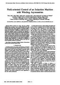
speed, which is directly applied by the pedal of the vehicle. Control is carried out by hysteresis comparators and a switching logic table selecting the appropriate voltage inverter switching configurations [4]. Figure 1 gives the global configuration of a DTC scheme and also shows how the EV dynamics is taken into account. 3-Phase Inverter V+ +
+bat.
Braking Braking Chopper Chopper
Battery Battery
V- _
-bat.
Isa Isb Isc
λs* + _
Concordia Concordia Transform Transformation
ωr
Vsd Vsq Isd Isq
Vehicle Dynamics
ωr
Ubus
Encoder
S a , Sb , S c
ωr * +
Induction Motor
PI
_
Tem* +
λs_est
_
Tem_est
Stator Stator Flux Flux & & Torque Torque Esimator Estimator
Fig.1. DTC block diagram.
Sensor fault detection and isolation – SFDI SFDI is based on two parts. The first one generates sensor residuals. The second part detects and isolates the faulty sensors (current, voltage, or speed sensors).
EKF for residual generation In previous works, multi-observer schemes have been obtained for fault detection and isolation [8]. Unfortunately, these schemes cannot be implemented due to the limited sampling period even with recently developed digital signal processors. For that purpose, it has been adopted only one observer. In this context an EKF is adopted to obtain the system state variable estimates (stator flux and rotational speed) and to generate the current and the speed residuals [10]. The Kalman filter, is a special class of linear observer (deterministic type), derived to meet a particular optimality stochastic condition. The Kalman filter has two forms: basic and extended. The EKF can be used for nonlinear systems where the plant model is extended by extra variables, in our case by the mechanical speed [11]. In an induction motor drive, the Kalman filter is used to obtain unmeasured state variables (rotor speed ωr, rotor flux vector components λrα and λrβ) using the measured state variables (stator current is and voltage components Vs in the Concordia frame α-β). Moreover, it takes into account the model and measurement noises. The induction motor state model used by the EKF is developed in the stationary reference frame and summarized by equation (1) [4], [10], where R is the resistance, L is the inductance, Lm is the magnetizing inductance. The implementation of the Kalman filter is based on a recursive algorithm minimizing the error variance between the real variable and its estimate.
⎧ ⎡ KR 0 ⎪ ⎢− K L ⎪ ⎢ ⎪ ⎡isα ⎤ ⎢ KR ⎪ ⎢i ⎥ ⎢ 0 − KL ⎪ ⎢ sβ ⎥ ⎢ d ⎪ ⎢λ rα ⎥ = ⎢ Lm 0 ⎪⎪ dt ⎢ ⎥ ⎢ ⎨ ⎢λ rβ ⎥ ⎢ Tr ⎪ ⎢ω ⎥ ⎢ Lm ⎪ ⎣ r ⎦ ⎢ 0 Tr ⎢ ⎪ ⎢ 0 ⎪ 0 ⎣ ⎪ ⎪ K L ⎛ Rs 1 − σ ⎞ =⎜ + ⎪ ⎟ , Tr = ⎪⎩ K R ⎝ Ls σTr ⎠
Lm Rr Lm ωr ⎤ 0 L2r K1 Lr K L ⎥ ⎥ Lm ωr Lm Rr ⎥ ⎡isα ⎤ ⎡1 0 ⎤ 0⎥ ⎢ ⎥ ⎢0 1 ⎥ Lr K L L2r K1 ⎥ ⎢isβ ⎥ ⎢ ⎥ ⎡Vsα ⎤ 1 ⎥ ⎢λ rα ⎥ + 0 0⎥ ⎢ ⎥ 1 ⎢ − −ωr 0 ⎥ ⎢ ⎥ K L V ⎢ 0 0 ⎥ ⎣ sβ ⎦ Tr ⎥ ⎢ λ rβ ⎥ ⎢ ⎥ ⎥ ⎢ω ⎥ ⎣0 0 ⎦ 1 0⎥ ⎣ r ⎦ ωr − Tr ⎥ 0 0 1 ⎥⎦
(1)
Ls L2m Lr , Ts = and σ = 1 − Rr Rs Ls Lr
Let us consider a linear stochastic system whose discrete state model is given by: ⎧⎪ x ( k + 1) = Ax ( k ) + Bu ( k ) + w ( k ) ⎨ ⎪⎩ y ( k + 1) = Cx ( k ) + v ( k )
(2)
where w(k) represents the disturbances vector applied to the system inputs. It also represents the modeling uncertainties; v(k) corresponds to system output measurement noises. It is supposed that the random signals v(k) and w(k) are Gaussian noises not correlated and with null average value. They are characterized by covariance matrixes, Q and R respectively, which are symmetrical and positive definite. The initial state vector x0 is also a random variable with covariance matrix P0 and average value x0 . The Kalman filter recursive algorithm is illustrated by Fig. 2.
u
y
System + _ B
+
C
+ A Q R
z-1
+
+
K
⎧ P(k + 1 k ) = A P(k k ) AT + Q ⎪⎪ −1 T T ⎨ K (k + 1) = P ( k + 1 k ) C [C P (k + 1 k ) C + R ] ⎪ ⎪⎩ P (k + 1 k + 1) = [ I n − K (k + 1) C ] P (k + 1 k )
Fig. 2. The Kalman filter recursive algorithm. For an induction motor, the Kalman filter must be used in its extended version. Therefore, a nonlinear stochastic system discrete state equation is given by:
⎧ xk +1 = f ( xk , uk ) + wk ⎨ ⎩ yk = h( xk ) + vk
(3)
where f and h are vector functions.
⎧ ⎡⎛ ⎤ Lm Rr Lm ωr KR ⎞ 1 Vsα ⎥ λ rβ + T ⎪ ⎢⎜ 1 − T ⎟ isα + T 2 λ rα + T KL ⎠ Lr K1 Lr K L KL ⎪ ⎢⎝ ⎥ ⎪ ⎢⎛ ⎥ ⎪ ⎢⎜ 1 − T K R ⎞⎟ isβ − T Lm Rr λ rα + T Lm ωr λ rβ + T 1 Vsβ ⎥ ⎪ ⎢⎝ ⎥ KL ⎠ L2r K1 Lr K L KL ⎪ ⎢ ⎥ ⎛ ⎪ 1⎞ ⎢ Lm ⎥ isα + ⎜ 1 − T ⎟ λ rα − T ωr λ rβ ⎪ f = ⎢T ⎥ T Tr ⎠ ⎨ ⎝ ⎢ r ⎥ ⎪ ⎢ L ⎥ ⎛ ⎞ 1 ⎪ ⎢T m isβ + T ωr λ rα + ⎜1 − T ⎟ λ rβ ⎥ ⎪ Tr ⎠ ⎢ Tr ⎥ ⎝ ⎪ ⎢ ⎥ ⎪ ⎣ ωr ⎦ ⎪ ⎡isα ⎤ ⎪h = C x = ⎢i ⎥ d k k 1 + ⎪ ⎣ sβ ⎦ ⎩ The notation k + 1 is related to predicted values at (k + 1)th instant and is based on measurements up to kth instant. T is the sampling period. The EKF equations are similar to those of the linear Kalman filter with the difference that A and C matrices should replaced by the Jacobians of the vector functions f and h at every sampling time as follows. ⎧ ∂f i ⎪ Ak [i, j ] = ∂x j x = xˆ(k k ) ⎪ ⎨ ∂hi ⎪ ⎪Ck [i, j ] = ∂x x = xˆ (k k − 1) j ⎩
(4)
The covariance matrices Rk and Qk are also defined at every sampling time. For the induction motor control, the EKF is used for the speed real-time estimation. It can also be used to estimate states and parameters using the motor voltages and currents measurements.
Sensor fault detection and isolation Current sensor faults
Three sensors are used to measure the motor currents. To detect current sensor faults, the following equation is used. isum = iasm + ibsm + icsm
(5)
Indeed, if one or two sensors fail, isum will be a non-zero sinusoidal signal. Therefore, additional logic and information (redundancy) are required to isolate the failed sensor. The required redundancy can be obtained from the EKF which is driven by the scheduled test input sets: ⎧TIS (1) = {iasm , ibsm , icsm1} when icsm1 = − ( iasm + ibsm ) ⎪ ⎨ m m2 m m2 m m ⎪⎩TIS ( 2 ) = {ias , ibs , ics } when ibs = − ( ias + ics )
(6)
TIS (1) is used to isolate a faulty current sensor in phase c and TIS (2) is used to isolate a faulty current sensor in phase a or b. It should be noticed that the two current residuals are calculated using Concordia components to isolate the faulty current sensor.
Voltages sensor faults
The fault detection may be performed using a simple threshold test on the parity equation (7), which describes the three-phase simple voltage equivalence. Vsum = Vasm + Vbsm + Vcsm
(7)
Speed sensor faults
The fault detection is achieved by comparing the measured speed with the estimated one. The encoder fault detection is given by the following residual. ˆ mm rϖ = ϖ mm − ϖ
(8)
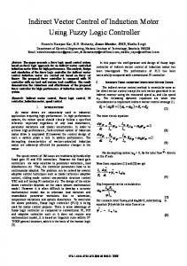
Figure 3 illustrates the SFDI principle. It includes the EKF, the residual generation and the Concordia transforms. Vαs iαs iβ s λαs λβs
EKF
iβ
i1αs or i2αs
i1βs or i2βs ˆm ω
Fault Isolation & Switching
iα
Residual Generation
Concordia Transform
iα
ˆr ω
Sensor (a) fault Sensor (b) fault Sensor (c) fault Sensor fault indicator Speed sensor fault
Vas
Vβs
Vbs Vcs imas imbs
icsm1 = − ( iasm + ibsm ) imas
ibsm 2 = − ( iasm + icsm ) imcs
iasm3 = − ( ibsm + icsm ) imbs
iβ
imcs
ωm
Fault Detection
Vas Vbs Vcs imas imbs imcs
Fig. 3. Sensor fault detection and isolation scheme.
Sensor fault-tolerant control scheme Figure 4 describes the proposed fault-tolerant control scheme in terms of current, voltage, and speed sensor faults.
Validation results Induction motor sensor fault-tolerant control Experimental tests have been first carried-out to check the sensor fault-tolerant control performances on a 1-kW induction motor drive (Fig. 5). Figures 6 and 7 show experimental results for current and speed sensors, respectively. The obtained results confirm the effectiveness of the proposed FTC approach.
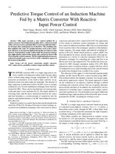
EV sensor fault-tolerant control The induction motor-based EV fault-tolerant control performances are then evaluated on a European urban and extra urban driving cycle. For that purpose, two sensor faults are introduced: a current sensor fault in phase a (an offset) at 2-sec and a speed sensor fault (a signal disconnection) at 7-sec. Figure 8 show the fault-tolerant performances in term of speed (via a single gear).
3-Phase Inverter
Induction Motor
Sa , Sb , S c
Vehicle Dynamics
λs*
_
λs_est
Vcs Vbs Vas
ics ibs ias
iαs
ω*
+
ωm
_
Tem*
PI
+
_
Tem_est
Current, Voltage, and Speed Sensor Fault Detection & Isolation
Iβs λαs λβs
SFDI
ωr Encoder
+
EKF
ωr_EKF
ωr
Fig. 4. The proposed sensor fault-tolerant control scheme.
Gearbox Wheel Induction Motor
Sa,Sb,Sc Control Unit Scope
Analog Output
Power Control Interface
Sensor Interface
Digital Output
TMS320F2407 DSP Development Board
Fig. 5. Schematic description of the experimental bench.
(Sensor fault indicator (green), Motor speed (orange), Speed sensor output (blue), Reference speed (Purple))
Fig. 6. Induction motor drive FTC performance under a current sensor fault.
Fig. 7. Induction motor drive FTC performance under a speed sensor fault. 160
140
Induction motor speed (rad/sec)
120
100
80
60
40
20
0
-20
× 10
0
2
4
6
8
10
12
14
16
18
20
Time (sec)
Fig. 8. EV FTC performances: Measured speed (red), Estimated speed (blue), and Reference speed (green).
Conclusion This paper dealt with a fault-tolerant control for an induction motor-based EV experiencing sensor faults (current, voltage, and speed). The carried-out simulations and experiments confirm that the proposed sensor FTC approach is effective and provides a simple configuration with high performance in term of speed response. Moreover, the obtained results show the global consistency and effectiveness of the proposed FTC strategy in comparison to previous studies, even with other type of electric propulsions [2].
References [1] Campos-Delgado D.U. et al.: Fault-tolerant control in variable speed drives: a survey, IET Electric Power Applications, vol.2, n°2, pp. 121-134, March 2008.
[2] Benbouzid M.E.H. et al.: Advanced fault-tolerant control of induction-motor drives for EV/HEV traction applications: From conventional to modern and intelligent control techniques, IEEE Trans. Vehicular Technology, vol. 56, n°2, pp. 519-528, March 2007. [3] Benbouzid M.E.H. et al.: Electric motor drive selection issues for HEV propulsion systems: A comparative study, IEEE Trans. Vehicular Technology, vol. 55, n°6, pp. 1756-1764, November 2006. [4] Tabbache B. et al.: An adaptive electric differential for electric vehicles motion stabilization, IEEE Trans. Vehicular Technology, vol. 60, n°1, pp. 104-110, January 2011. [5] Lee K.S. et al.: Instrument fault detection and compensation scheme for direct torque controlled induction motor drives, IEE Proc. Control Theory Applications, vol. 150, n°4, pp. 376-382, July 2003. [6] Rothenhagen K. et al.: Doubly fed induction generator model-based sensor fault detection and control loop reconfiguration, IEEE Trans. Industrial Electronics, vol. 56, n°10, pp. 4229-4238, October 2009. [7] Rothenhagen K. et al.: Current sensor fault detection, isolation, and reconfiguration for doubly fed induction generators, IEEE Trans. Industrial Electronics, vol. 56, n°10, pp. 4239-4245, October 2009. [8] Bennett S.M. et al.: Sensor fault-tolerant control of a rail traction drive, Control Engineering Practice, vol. 7, n°2, pp. 217-225, February 1999. [9] Akrad A. et al.: Design of a fault-tolerant controller based on observers for a PMSM drive, IEEE Trans. Industrial Electronics, vol. 58, n°4, pp. 1416-1427, April 2011. [10] Akın B. et al.: Simple derivative-free nonlinear state observer for sensorless AC drives, IEEE/ASME Trans. Mechatronics, vol. 11, n°5, pp.1083-4435, October 2006. [11] Harnefors L.: Instability phenomena and remedies in sensorless indirect field oriented control, IEEE Trans. Power Electronics, vol. 15, n°4, pp. 733-743, July 2002.