2000). Global stabilization of the zero solution of the KSE (e.g., Christofides and Armaou, SCL, 2000). Boundary control (e.g., Liu ... xs(t) = Psx(t), xf (t) = Pf x(t).
OPTIMAL ACTUATOR/SENSOR PLACEMENT FOR NONLINEAR CONTROL OF THE KURAMOTO-SIVASHINSKY EQUATION
Yiming Lou and Panagiotis D. Christofides
Department of Chemical Engineering University of California, Los Angeles
KURAMOTO-SIVASHINSKY EQUATION • Kuramoto-Sivashinsky equation with distributed control: l
∂U ∂4U ∂2U ∂U X bi ui (t) = −ν 4 − −U + ∂t ∂z ∂z 2 ∂z i=1
• Boundary conditions:
∂j U ∂j U (−π, t) = (+π, t) , j = 0, . . . , 3 ∂z j ∂z j
• The stability of steady-state U (z, t) = 0 depends on ν.
INTRODUCTION • Important systems described by the Kuramoto-Sivashinsky equation: ¦ Falling liquid films. ¦ Unstable flame fronts. ¦ Interfacial instabilities between two viscous fluids. • Feedback control of the Kuramoto-Sivashinsky equation: ¦ Finite-dimensional output feedback controller design based on Galerkin’s method (e.g., Armaou and Christofides, CES and Physica D, 2000). ¦ Global stabilization of the zero solution of the KSE (e.g., Christofides and Armaou, SCL, 2000). ¦ Boundary control (e.g., Liu and Krstic, NA, 2001). • Optimal actuator/sensor placement for the Kuramoto-Sivashinsky equation?
BACKGROUND ON ACTUATOR/SENSOR PLACEMENT • Optimal actuator placement for linear controllers and PDE models. ¦ Controllability measures (e.g., Arbel, 1981). ¦ Optimal controller gain/actuator location to minimize cost on system response and control action (e.g., Rao et al, AIAA J., 1991). • Optimal sensor placement for linear estimators and PDE models. ¦ Observability measures (e.g., Yu and Seinfeld, IJC. 1973; Waldraff et al, JPC, 1998). ¦ Minimum estimation error under worst measurement noise (e.g., Kumar and Seinfeld, IEEE TAC, 1978; Morari and O’Dowd, Automatica 1980). Review paper: Kubrusly and Malebranche, Automatica, 1985. • Optimal actuators/sensors placement for nonlinear dissipative PDE systems (Antoniades and Christofides, C&CE, 2000; CES, 2001; C&CE, 2002).
PRESENT WORK (Lou and Christofides, IEEE CST, 2002) • Optimal actuator/sensor placement for nonlinear control of the Kuramoto-Sivashinsky equation. ¦ Order reduction using linear/nonlinear Galerkin’s method. ¦ Computation of optimal location of actuators and sensors through minimization of a cost that includes penalty on the closed-loop response and the control effort. ¦ Nonlinear output feedback controller design using geometric methods. • Illustration of theoretical results through computer simulation of the closed-loop system using a high-order discretization of the KSE.
KURAMOTO-SIVASHINSKY EQUATION • Kuramoto-Sivashinsky equation with distributed control: l
∂U ∂4U ∂2U ∂U X −U = −ν 4 − + bi ui (t) ∂t ∂z ∂z 2 ∂z i=1 ∂j U ∂j U (−π, t) = (+π, t) , j = 0, . . . , 3 ∂z j ∂z j
• Boundary conditions:
• Representation in Hilbert space: x=Ax ˙ + Bu + f (x), x(0) = x0 ym =kx A: linear operator. f (x): nonlinear function.
EIGENSPECTRUM / OPEN-LOOP DYNAMICS • Eigenvalue problem: Aφn
• Eigenvalues:
∂ 4 φn ∂ 2 φn − = λn φn , n = 1, . . . , ∞ = −ν ∂z 4 ∂z 2 ∂ j φn ∂ j φn (−π) = (+π) , j = 0, . . . , 3 j j ∂z ∂z
λn = −νn4 + n2 , n = 1, . . . , ∞:
Structure of Eigenspectrum
Open-loop profile of U (z, t)
Im
6 4 2
U
ν = 0.2 −35.2
−7.2
0.8
Re
ν = 0.2
0 −2 −4 −6 0 2
3 2 4
1 0 6
−1 −2
t
8
−3 z
GALERKIN’S METHOD • Hs = span{φ1 , φ2 , . . . , φm }, Hf = span{φm+1 , φm+2 , . . . , }. xs (t) = Ps x(t),
xf (t) = Pf x(t)
Ps , Pf : orthogonal projection operators. • Set of infinite ODEs. dxs dt ∂xf ∂t
=
As xs + bs u + fs (xs , xf )
=
Af xf + bf u + ff (xs , xf )
• Finite-set of ODEs. d˜ xs dt
= As x ˜s + Bs u + fs (˜ xs , 0)
• Order reduction using Galerkin’s method and approximate inertial manifolds is also possible.
NONLINEAR CONTROL DESIGN d˜ xs dt
=
As x ˜s + Bs u + fs (˜ xs , 0)
• Assumption: l = m (i.e. number of manipulated inputs is equal to the number of slow modes) and Bs is invertible. • Nonlinear state feedback controller: u =
Bs−1 ((Λs − As )˜ xs − fs (˜ xs , 0)) Λs is a stable matrix.
• Closed-loop ODE system: x ˜˙ s = Λs x ˜s • Response depends on Λs and xs (0), but not on actuator locations: x ˜s = eΛs t xs (0)
OPTIMAL POINT ACTUATOR PLACEMENT • Performance criterion (sum is over a set of m linearly independent xis (0)): Jˆs
=
m Z ∞ X 1 ((˜ xs (xis (0), t), Qs x ˜s (xis (0), t)) m i=1 0
+uT (˜ xs (xis (0), t), za )Ru(˜ xs (xis (0), t), za ))dt • However, system’s response does not depend on the actuator locations: m Z ∞ X 1 Jˆxs = (˜ xs (xis (0), t), Qs x ˜s (xis (0), t))dt m i=1 0 • Performance criterion reduces to: m Z ∞ X 1 Jˆus = uT (˜ xs (xis (0), t), za )dt xs (xis (0), t), za )Ru(˜ m i=1 0 • Computation of optimal actuator locations: " #T ∂ Jˆus ∂ Jˆus ∂ Jˆus ... = [0 0 ∂za1 ∂za2 ∂zal
...
• Near-optimal solution for distributed system as ² =
T 0] , ∇za za Jˆus (zam ) > 0
|λ1 | |λm+1 |
→ 0.
OPTIMAL LOCATION OF POINT SENSORS d˜ xs dt y˜m
=
As x ˜s + Bs u + fs (˜ xs , 0)
=
Sx ˜s
• Assumption: p = m(i.e. the number of sensors is equal to the number of slow modes) and S is invertible. • Computation of estimate of x ˜s from the measurements: x ˆs = S −1 ym ym : sensor measurements, x ˆs estimate of x ˜s . • Compute point sensor locations to minimize the estimation error in the closed-loop system: m Z ∞ X 1 ˆ J(e) = (||xs (xis (0), t) − x ˆs (xis (0), t)||2 )dt m i=1 0 xs : slow state of infinite set of ODEs,
e(t) = ||xs − x ˆs ||2
• Near-optimal solution for distributed system as ² → 0.
KURAMOTO-SIVASHINSKY EQUATION • Kuramoto-Sivashinsky equation with distributed control: l
∂U ∂4U ∂2U ∂U X bi ui (t) = −ν 4 − −U + ∂t ∂z ∂z 2 ∂z i=1
• Boundary conditions:
∂j U ∂j U (−π, t) = (+π, t) , j = 0, . . . , 3 ∂z j ∂z j
• The stability of steady-state U (z, t) = 0 depends on ν.
CONTROLLER SYNTHESIS Kuramoto-Sivashinsky equation, ν = 0.2 • ν = 0.2 → Two unstable eigenmodes. • Order of ODE model used for controller design:2 Number of control actuators:2; Number of measurement sensors:2 • Approximate two-dimensional ODE system used for controller design. " # " #" # (x ˜˙ s1 , φ1 ) (x ˜˙ s2 , φ2 )
=
λ1
0
(˜ xs1 , φ1 )
0
λ2
(˜ xs2 , φ2 )
#"
" +
φ1 (za1 )
φ1 (za2 )
u1
φ2 (za1 )
φ2 (za2 )
u2
#
" +
#
(f1 (˜ xs , 0), φ1 ) (f2 (˜ xs , 0), φ2 )
za1 , za2 : location of point actuators.
CONTROLLER SYNTHESIS • Nonlinear state feedback controller: " # " u1 u2
=
φ1 (za1 )
φ1 (za2 )
φ2 (za1 )
φ2 (za2 )
#−1
#"
Ã" ∗
−α − λ1
0
(˜ xs1 , φ1 )
0
−β − λ2
(˜ xs2 , φ2 )
" −
#
#! (f1 (˜ xs , 0), φ1 ) (f2 (˜ xs , 0), φ2 )
α and β are positive real numbers. • The structure of the closed-loop finite-dimensional system under the feedback control : " # " #" # (x ˜˙ s1 , φ1 ) (x ˜˙ s2 , φ2 )
=
−α
0
(˜ xs1 , φ1 )
0
−β
(˜ xs2 , φ2 )
which is independent of the actuator locations.
OPTIMAL LOCATION OF ACTUATORS • Cost for optimal location of control actuators: Jˆs
=
2 Z X 1
2
i=1
∞
((˜ xTs (xis (0), t), Qs x ˜s (xis (0), t)) 0
+uT (˜ xs (xis (0), t), za )Ru(˜ xs (xis (0), t), za ))dt
#
" Qs = R =
1
0
0
1
, x1s (0) = [ φ1
2 0 ], xs (0) = [ 0
φ2 ].
Optimal actuator locations: za1 = 0.31π and za2 = 0.69π.
OPTIMAL LOCATION OF SENSORS • Cost for optimal location of measurement sensors: ˆ = J(e)
2 Z X 1
2
∞
(||xs (xis (0), t) − x ˆs (xis (0), t)||2 )dt
0
i=1
where xs can be obtained from the simulation of the high order system, and x ˆs is calculated from the output: "
# x ˆs1 x ˆs2
" =
#" φ1
0
φ1 (zs1 )
φ1 (zs2 )
0
φ2
φ2 (zs1 )
φ2 (zs2 )
#−1 "
Optimal sensor locations: zs1 = 0.35π and zs2 = 0.64π.
# ym1 (zs1 , t) ym2 (zs2 , t)
SIMULATION RESULTS • State feedback control with two actuators. Case
Actuator locations
Jˆs
Optimal
.31π, .69π
3.3705
2
.30π, .80π
4.1536
3
.40π, .60π
5.2238
4
.20π, .80π
5.1089
• Closed-loop norm of ||u|| for the optimal case (solid line), case 2 (long-dashed line), case 3 (short-dashed line), and case 4 (dotted line). Left plot: xs (0) = [ φ1 0 ]. Right plot: xs (0) = [ 0 φ2 ].
10
10
||u||
15
||u||
15
5
0
5
0
1
2
3
4 t
5
6
7
8
0
0
1
2
3
4 t
5
6
7
8
SIMULATION RESULTS • Output feedback control with two sensors (optimal actuator locations). Case
Sensor locations
ˆ J(e)
Jˆs
Optimal
.35π, .64π
2.86e-4
3.8748
2
.20π, .80π
1.841e-3
3.8830
3
.20π, .50π
5.020e-3
3.9273
• Closed-loop norm of the closed-loop estimation error kek versus time, for the optimal actuator/sensor locations. Dotted line: xs (0) = [ φ1 0 ]. Solid line: xs (0) = [ 0 φ2 ]. −4
7
x 10
6
5
e
4
3
2
1
0
0
1
2
3
4 t
5
6
7
8
SIMULATION RESULTS • Profiles of the evolution of U under output feedback control, for optimal actuator/sensor locations, for xs (0) = [ φ1 0 ] (left figure), and xs (0) = [ 0
φ2 ] (right figure).
0.6 0.6
0.4 0.4
0.2 0.2
0 U
0 U
−0.2
−0.2
−0.4
−0.4
−0.6
−0.6
−0.8 0
−0.8 0
2
3
2
3
2 4
1
2 4
1 0
0 6
6
−1
t
8
−1 −2
−2 −3 z
t
8
−3 z
SIMULATION RESULTS • Profiles of KSE under output feedback control, for the optimal actuator/sensor locations, for xs (0) = [ φ1 0 ] and uncertainty in ν. Manipulated input profiles - Solid line u1 and dashed line u2 0.5
0 0.6 0.4
−0.5 0.2
U
u1, u2
0 −0.2
−1
−0.4
−1.5
−0.6 −0.8 0 5
3
−2
2 10
1 0 15
−1 −2
t
20
−2.5
−3 z
0
2
4
6
8
10 t
12
14
16
18
20
SIMULATION RESULTS • Profiles of KSE under output feedback control, for the optimal actuator/sensor locations, for xs (0) = [ 0 φ2 ] and uncertainty in ν. Manipulated input profiles - Solid line u1 and dashed line u2 2
1.5
0.6
1
0.4
0.5
0.2
U
u1, u2
0 −0.2 −0.4
0
−0.5
−0.6
−1
−0.8 0 10
3
20
−1.5
2 30
1 0
40
−1
50 t
−2
−2 60
0
10
20
30
−3 z
t
40
50
60
CONCLUSIONS • Optimal actuator/sensor placement for nonlinear control of the KSE. ¦ Order reduction using Galerkin’s method ¦ Nonlinear output feedback controller design using geometric methods. ¦ Computation of optimal actuator/sensor location through minimizing a cost that includes penalty on the close-loop response and control effort. ACKNOWLEDGMENT • Financial support from the National Science Foundation, CTS-0002626, and the Air Force Office of Scientific Research is gratefully acknowledged.