Separable Approximate Optimization of Support

Separable Approximate Optimization of Support Vector Machines for Distributed Sensing Sangkyun Lee, Marco Stolpe, and Katharina Morik Fakult¨ at f¨ ur Informatik, LS VIII Technische Universit¨ at Dortmund 44221 Dortmund, Germany {sangkyun.lee,marco.stolpe,katharina.morik}@tu.dortmund.de

Abstract. Sensor measurements from diverse locations connected with possibly low bandwidth communication channels pose a challenge of resource-restricted distributed data analyses. In such settings it would be desirable to perform learning in each location as much as possible, without transferring all data to a central node. Applying the support vector machines (SVMs) with nonlinear kernels becomes nontrivial, however. In this paper, we present an efficient optimization scheme for training SVMs over such sensor networks. Our framework performs optimization independently in each node, using only the local features stored in the respective node. We make use of multiple local kernels and explicit approximations to the feature mappings induced by them. Together they allow us constructing a separable surrogate objective that provides an upper bound of the primal SVM objective. A central coordination is also designed to adjust the weights among local kernels for improved prediction, while minimizing communication cost. Keywords: distributed features, support vector machines, separable optimization, primal formulation, approximate feature mappings

1

Introduction

Sensor networks have been a very active research topic in recent machine learning and data mining [12, 13]. Sensors are adopted to monitor certain aspects of objects or phenomena that we are interested in, often located in such places hardly accessible by human beings. Various applications include factory control, traffic monitoring, and climate warning, where sensors must communicate with each other or with a central arbitrator in order to provide useful information for decision making. Challenges arise in sensor networks when we try to build a predictor collecting information from all sensors, where sensors can afford only minimal communication due to their distance to a central station or low-power requirements. If this is the case, we might prefer to perform learning in a distributed fashion, where each separated part of learning relies on the locally stored measurements only. It will require, however, a learning approach whose computation can be

2

S. Lee, M. Stolpe and K. Morik

distributed in a well-defined way, equipped with a global arbitration that can maximize prediction performance without incurring too much information transfer from sensors. In this paper we suggest a variant of the support vector machines (SVMs) using nonlinear kernels on sensor data. We define kernels that use only locally stored features in sensors, computing explicit forms of approximations to the feature mappings that correspond to each local kernel. For typical error functions for SVMs, we then create a separable surrogate objective function that forms an upper bound on the original primal SVM objective. Each separated part in the objective is designed to use a single local kernel, and therefore can be optimized locally at the sensors. We also provide an additional central optimization that uses inner product results from the sensors, without requiring an access to local kernel functions or their approximations. The central optimization provides local kernels new weights, that can be fed to the sensors and generate possibly improved local solutions.

2

Separable Optimization

In this section we begin with a general description of the support vector machines (SVMs), shaping it progressively to a form which can be optimized separately for local features in each network node. 2.1

Support Vector Machines

We consider a given data set {(xi , yi )}m i=1 which consists of pairs of input feature vectors xi ∈ Rp and their labels yi , where yi ∈ {−1, +1} for classification and yi ∈ R for regression. The SVMs for 1- and 2-class classification and regression can be formulated as an unconstrained convex minimization, min w∈H,ρ∈R

m " 1 # λ! 2 #w#H + ρ + # ($w, φ(xi )%, yi , ρ) 2 m i=1

(1)

where λ > 0, and the convex loss function # and the scalar ρ are chosen by the task of interest, as in Table 1. For readability we ignore the intercept term of a decision plane without loss of generality, which can be easily included by augmenting vectors w and x. We call φ : Rp → H, for a Hilbert space H, a feature mapping induced by a positive semidefinite kernel k, with the relation that k(xu , xv ) = $φ(xu ), φ(xv )%. 2.2

Multiple Localized Kernels

Now, we consider that the input features are stored in a distributed fashion among n nodes, possibly with overlaps among them. We suppose that there are p unique features in total, denoting the subset of feature indices stored in the

Separable Optimization of SVMs for Distributed Sensing

3

Table 1. The choices of the loss function ! and a scalar ρ in the canonical objective of SVMs in the equation (1). Setting ρ = 0 implies we essentially ignore ρ in optimization. Task !(zi , yi , ρ) range of ρ Classification (1-class) max{0, ρ − zi } R Classification (2-class) max{0, 1 − yi zi } 0 Regression max{0, |yi − zi | − #} 0

jth node by Sj ⊂ {1, 2, . . .$ , p}, and its cardinality by pj := |Sj | > 0, so that n ∪nj=1 Sj = {1, 2, . . . , p} and j=1 pj ≥ p. For convenience, we refer to the feature subvector of xi stored in the jth node as xi [j] ∈ Rpj . For each node we make use of an individual kernel which depends on only the features stored locally in nodes. We denote the kernel for the jth node by kj : Rpj ×pj → R and its corresponding feature mapping by φj : Rpj → Hj . Then we can construct a composite kernel k as a conic combination of local kernels, that is, k(xu , xv ) :=

n # j=1

µ2j kj (xu [j], xv [j]), ∀u, v ∈ {1, 2, . . . , m}.

(2)

(It will become clear why we use µ2j rather than µj ≥ 0, as we progress.) The weights for local kernels µj will be optimized, which defines our central optimization problem to be discussed later. This setting is very similar to the multiple kernel learning (MKL) and boosting, but our resulting framework will not be exactly the same, as we discuss later in Section 3. We note that using multiple kernels alone does not lead to a separable objective for SVMs. From the representer theorem [19], the optimal weight w of SVM (1) is expressed as a linear span of the representers k(xi , ·). That is, w(·) =

m # i=1

(2)

αi k(xi , ·) =

n #

µ2j

j=1

m # i=1

αi kj (xi [j], ·[j]),

(3)

Replacing w into (1) results in the following objective:   n m m m n m λ # 2## 1 # # 2 # min µj αu αv kj (xu , xv )+ # µj αu kj (xu , xi ), yi , ρ . α∈Rm 2 m i=1 u=1 v=1 u=1 j=1 j=1

We can see all optimization variables α1 , α2 , . . . , αm are coupled with each node j = 1, 2, . . . , n, therefore cannot be split over nodes. This also indicates that we would need alternative ways to incorporate kernels rather than relying on the representer theorem, to achieve separability. 2.3

Approximating Feature Mappings

One observation of the original SVM formulation (1) is that the terms #w#2 and $w, φ(xi )% would be separable over the components of w, if w was in a finite

4

S. Lee, M. Stolpe and K. Morik

dimensional space1 . Motivated by this, we introduce explicit finite-dimensional approximations to the feature mappings φ ∈ H that correspond to kernel functions k(x, x# ) = $φ(x), φ(x# )%. This step is necessary, since the explicit form of φ is unavailable in general. For each node j, suppose that we have obtained an approximate feature mapping ϕj : Rpj → Rdj to the original mapping φj , where dj ∈ (0, ∞) is a predefined (possibly small) integer, so that $ϕj (x[j]), ϕj (x# [j])% ≈ kj (x[j], x# [j]) = $φ(x[j]), φ(x# [j])%. $n If d := j=1 dj is sufficiently large, we can consider the following d-dimensional approximation problem to the original SVM (1): min

w∈Rd ,ρ∈R

m " " 1 # ! T λ! #w#22 + ρ + # w ϕ(xi ), yi , ρ . 2 m i=1

(4)

Regarding the representation (3), we impose a weight for the feature mappings for every node:     w[1] µ1 ϕ1 (xi [1]) n  w[2]   µ2 ϕ2 (xi [2])  #     T µj w[j]T ϕj (xi [j]). ϕ(xi ) :=   , w :=  ..  ⇒ w ϕ(xi ) = ..  .    . j=1 w[n] µn ϕn (xi [n]) (5) Here we denote by w[j] ∈ Rdj the subvector of w ∈ Rd for the node j. Again, by xi [j] ∈ Rpj we denote the attributes of xi ∈ Rp stored in the node j. In the expansion for wT ϕ(xi ) above, we have µj but no µ2j as in (2) or (3). The reason is that we do not have any inner product between images of ϕj (·): this becomes a crucial property for deriving a separable optimization problem. There have been largely two types of approaches to find approximate feature mappings ϕ. The first type of approaches is based on computing low-rank factor matrices that approximate the original kernel matrices [4, 3, 6]. Although this type allows to use any positive semidefinite kernel matrices, it requires matrix factorization with comparably large memory footprint. In the second type, we make use of random projections and construct approximate mappings directly [16]. These methods tend to require larger approximation dimensions than the first type [11], but they are much simpler and easier to parallelize. In this paper we focus on the second type approximation of Gaussian kernels k(xu , xv ) = exp(−γ#xu − xv #22 ) without loss of generality, for which the approximation is given by / 1T 2 0 ϕj (x[j]) = cos(zT1 x[j] + e1 ), cos(zT2 x[j] + e2 ), . . . , cos(zTdj x[j] + edj ) , dj (6) 1

The loss functions ! in Table 1 are not separable as well. We will discuss them as a next step in the following section.

Separable Optimization of SVMs for Distributed Sensing

5

for each node j, where zk ∈ Rpj and ek ∈ R are i.i.d. random samples from the Gaussian distribution N (0, 2γI), I is an identity matrix, and from the uniform distribution on [0, 2π], respectively. These are derived from the Fourier transform of the kernel function kj (for more details see [16]). Note that ϕj uses only local features stored in the jth node, represented as a subvector x[j]. 2.4

A Separable Surrogate Objective

Our final step is to make the loss functions # in Table 1 separable over nodes, using their convexity $ in the first and the last arguments. Without loss of genern ality, we impose that i=1 µj = 1 in addition to µj ≥ 0. Then we can derive an upper bound for the hinge loss # of 2-class classification tasks as follows, #(wT ϕ(xi ), yi , ρ) = max{0, 1 − yi wT ϕ(xi )} n # = max{0, µj (1 − yi w[j]T ϕj (xi ))} j=1

≤

n # j=1

µj max{0, 1 − yi w[j]T ϕj (xi ))}

(7)

where #j is listed in the second row of Table 2. Upper bounds for 1-class classification and regression tasks can be derived similarly and are$presented in the n table as well. (For 1-class problems, we define ρj so that ρ = j=1 µj ρj .) Summing the inequality (7) over training indices i = 1, 2, . . . , m leads to an upper bound of the objective function in (4): m " " 1 # ! T λ! 2 #w#2 + ρ + # w ϕ(xi ), yi , ρ 2 m i=1 2 3 n m # " ! " λ! 1 # 2 T ≤ #w[j]#2 + µj ρj + µj #j w[j] ϕj (xi ), yi , ρj . 2 m i=1 j=1

(8)

The expression in the right hand side is separable in terms of nodes. Therefore, in each node we can solve the following separated problem for each node j = 1, 2, . . . , n, m

(Local)

min

w[j]∈Rdj ,ρj ∈R

" ! " 1 # λ! #w[j]#22 + µj ρj + µj #j w[j]T ϕj (xi ), yi , ρj . 2 m i=1

(9)

Although it is possible to construct a global classifier by transferring all solutions w∗ [j] and ρ∗j of (9) for j = 1, 2, . . . , n, it may not be desirable since then the central node should know about ϕj and the random basis vectors consisting it. Therefore, for a (test) vector x, whose components are assumed to be stored in a distributed fashion, each node can compute and transfer w∗ [j]T ϕj (x[j]) and $n ρ∗j to a central node, where the summations w∗ T ϕ(x) = j=1 µj w∗ [j]T ϕj (x[j]), $n and ρ∗ = j=1 µj ρj can be used for a global prediction.

6

S. Lee, M. Stolpe and K. Morik Table 2. The jth summand in the upper bounds for the loss functions. T Task !j (w[j] ϕj (xi ), yi , ρj ) " range of ρj ! Classification (1-class) max 0, ρj − w[j]T ϕj (xi ) R Classification (2-class) max{0, 1 − yi w[j]T ϕj (xi ))} 0 Regression max{0, |yi − w[j]T ϕ(xi )| − #} 0

2.5

Minimization of Approximation Gaps

We discuss the quality of two approximations we have made, in using approximate feature mappings and an inequality due to convexity of loss functions, to arrive the separated local optimization (9) from the nonseparable SVM formulation (1), assuming that both are using multiple localized kernels. Approximation in Feature Mappings The first approximation has been applied when we use approximate feature mappings in Section 2.3. In the case of the mapping ϕj : Rpj → Rdj in (6) approximating a local Gaussian kernel kj (x[j], x# [j]) = exp(−γj #x[j] − x# [j]#22 ), x[j] ∈ Rpj , the following result from [16] quantifies its quality: 3 2 5 66 5 4 4 1 2 dj T # # 4 4 , P sup ϕj (x[j]) ϕj (x [j]) − kj (x[j], x [j]) ≥ ) ≤ O 2 exp −) ) pj x[j],x! [j]∈M where M ⊂ Rpj is a compact set containing all subvectors xi [j], i = 1, 2, . . . , m. Therefore, ϕj will grants us good approximation as long as we use sufficiently large dj for its approximation dimension.

Approximation in the Convex Inequality Another approximation takes place in (7) and (8), where we construct separable upper bounds of the nonseparable loss # functions in Table 1. Since the inequality is constructed using the convex combination parametrized by µ1 , µ2 , . . . , µn , we can reduce the gap in the inequality by minimizing the right hand side expression of (8) in terms of µj ’s. This defines an optimization problem in a central node, m

n

1 ## Lij µj + Ψ (µ) µ:=(µ1 ,µ2 ,...,µn )T m i=1 j=1   n n n # # # (Central) subject to Lij µj ≥ #  Zij µj , yi , µj ρj  , min

j=1

n # j=1

j=1

(10)

j=1

µj = 1, µj ≥ 0, j = 1, 2, . . . , n.

Here we have defined 7 Zij := w[j]T ϕj (xi [j]) , i = 1, 2, . . . , m, j = 1, 2, . . . , n. Lij := #j (Zij , yi , ρj )

(11)

Separable Optimization of SVMs for Distributed Sensing

7

These remain constant in the central optimization (10), whose elements can computed in local nodes independently and transferred to a central node. The last term Ψ in the objective is an optional convex regularization term. This can be chosen as Ψ (µ) = σ#µ#22 for a given σ > 0 to produce a unique or an evenly distributed solution, Ψ (µ) = σ # #µ#1 to induce elementwise sparsity in µ (thereby selecting few local kernels important for prediction, similarly to MKL), $G or Ψ (µ) = σ ## g=1 #µ[g]#2 for subvectors µ[g] to promote groupwise sparsity (e.g. selecting few clusters of nodes, rather than individual nodes).

3

Related Works

We present two most closely related learning approaches to our framework. 3.1

Multiple Kernel Learning

The multiple kernel learning (MKL) is an extension of the support vector machines for employing multiple kernel functions, instead of a single one as in the standard settings. The current forms and efficient learning methods for MKL have been established in [10, 9, 1, 2]. In MKL we consider a combination of n kernels n # k(xu , xv ) = βj kj (xu , xv ), (12) j=1

$n

where βj ≥ 0, j=1 βj = 1, and kj are defined on a certain subset of features. Plugging the composite kernel k(xu , xv ) into the standard SVM formulation leads to a semi-definite program (SDP) [10], which is much harder to solve than the standard SVMs. When kernels kj are normalized, i.e. kj (x, x) = 1, it can be reduced to a quadratically constrained quadratic program [9], which can be solved slightly more efficiently than SDPs. Modifications to the SVM formulations lead to further improvement, resulting in a semi-infinite linear program [18], a quadratic program [17], and a much faster interleaved optimization using #p -norms [8]. The main difference of MKL to our framework is that the objective function of MKL is not separable over nodes. For instance, the MKL formulation in [17] solves the dual problem max − α

s.t.

n m m m # 1 # ## βj αu αv kj (xu , xv ) + αu 2 j=1 u=1 v=1 u=1

m #

u=1

αu yu = 0, 1/(mλ) − αu − νu = 0, ∀u = 1, 2, . . . , m.

Similar to our discussion in Section 2.2, all variables αu in this objective are coupled with each node j, therefore the optimization cannot be separated over nodes. Another difference is the ways to form convex combinations of kernels. 8 Comparing the convex combinations in (12) and (2), we can interpret µ as βj , j $n $n and our framework imposes j=1 µj = 1 rather than j=1 µ2j = 1.

8

3.2

S. Lee, M. Stolpe and K. Morik

Boosting

Boosting with an additive model [5] is also quite similar to our model and the MKL. In boosting, we find a linear combination of n basis functions or weak learners of the form n # h(x) = ζj hj (w; x), j=1

where ζj ∈ R and hj can be set hj (w; x) = w[j]T ϕj (x[j]) to resemble our setting. The optimal w∗ [j] can be found independently for each node j = 1, 2, . . . , n, and the best combination of hj ’s can be found as follows,   m n # # min # ζj hj (w∗ ; xi ), yi , ρ . n ζ:=(ζ1 ,...,ζn )∈R

i=1

j=1

This looks similar to our central problem (10). Despite its similarity, however, the objective of the central problem does not provide an upper bound of the MKL loss as in our formulation (7), thereby losing its connection to the MKL. Also, unlike our setting and MKL, the local problems in boosting do not depend on the weights ζj . That is, the solutions from separated problems cannot be improved any further through new weight values of ζj obtained from a central optimization. Our framework and MKL share the property that subproblem (separated problems in our case, and the nonseparable problem obtained after fixing weights in MKL) are dependent on such weights, therefore improved solutions can be obtained using adjusted weight values.

4

Algorithm

We describe our algorithm that solves the separated problem (9) at each local node, and the additional central optimization (10) that determines an optimal convex combination. The outline of the entire framework is presented in Algorithm 1. 4.1

Local Optimization

To find the solutions of each separated local optimization problem, we use the stochastic gradient descent (SGD) approach. In particular, we adapt the “robust” version of SGD suggested by Nemirovski and Yudin [15], for which a simplified analysis [14] or a regret-based online analysis [20] can be found. We sketch the robust SGD algorithm here and refer to the ASSET approach [11] for details, which implements essentially the same idea for the standard SVMs. To simplify our notation we denote the objective function of the jth separated local problem in (9) by fj : m

" ! " λ! 1 # fj (w[j], ρj ) := #w[j]#22 + µj ρj + µj #j w[j]T ϕj (xi ), yi , ρj . 2 m i=1

Separable Optimization of SVMs for Distributed Sensing

9

Algorithm 1: Separable SVM with Approximations to Local Kernels input : A data set {(xi , yi )}m i=1 , the number of iterations K (K > 1 only if we use central optimization), T , and T0 , and a constant µ0 > 0. Initialize: µj ← µ0 , for j = 1, 2, . . . , n; for k = 1, 2, . . . , K do Transmit µj to all nodes j = 1, 2, . . . , n; (local in parallel) // Solve a separated local problem in each node j, using ASSET input : a weight µj and local measurements {(xi [j], yi )}m i=1 . ¯ Initialize iterates and averages: w[j]1 ← 0, ρ1j ← 0 w[j] ← 0, ρ¯j ← 0; Estimate an optimization constant θj > 0; for t = 1, 2, . . . , T do Select a random training index ξt ∈ {1, 2, . . . , m}; √ Compute a steplength ηt = θj / t; t+1 Update w[j]t+1 and ρj via (13); end ¯ output: weighted averages of iterates, w[j] and ρ¯j , for the last (T − T0 ) iterations. ¯ T ϕj (xi ) for i = 1, 2, . . . , m and output: (optional) transfer Zij := w[j] ρ¯j to a central node. (end) (optional central) // Solve the additional central problem using CPLEX input : Zij and ρ¯j for i = 1, 2, . . . , m, j = 1, 2, . . . , n Compute Lij := # !j (Zij , yi , ρ¯j ) for all i = 1, 2, . . . , m, j = 1, 2, . . . , n; Compute ρ = n ¯j ; j=1 µj ρ Solve the equivalent formulation (14); output: new weights µ1 , µ2 , . . . , µn . (end) end

Then in each iteration of the local optimization, we update the variables w[j] and ρj as follows, 6 59 : 9 : w[j]t+1 w[j]t (13) − ηt Gt , t = 1, 2, . . . , T, ← PW ρtj ρt+1 j where PW (z) := arg minv∈W { 12 #z − v#22 } is an Euclidean projection of a vector z onto a convex set W, Gt is an estimate subgradient of fj at (w[j]t , ρtj ), constructed using a random training example chosen by ξt ∈ {1, 2, . . . , m}, and ηt √ is a steplength of the form ηt = θj / t for some θj > 0. The set W guides the optimization to avoid having new iterates with too large norm values, for which the formulation can be derived from strong duality. θ The convergence of the robust SGD algorithm is O(c(T0 /T ) √jT ) in terms of objective function values, where c(·) is a simple function depending on the ratio T0 /T only [14].

10

S. Lee, M. Stolpe and K. Morik

4.2

Central Optimization

The central problem (10), for the loss functions # in Table 1, can be formulated as a linear program (LP) or a quadratic program (QP) depending on the choices of the regularizer Ψ . When we consider 2-class problems with Ψ (w) = σ#w#22 for σ ≥ 0, we can write an equivalent formulation to (10) as follows, 1 (L1m )T µ + σµT µ, m s.t. (L + Dy Z)µ ≥ 1m , 1Tn µ = 1, µ ≥ 0.

min

µ∈Rn

(14)

where the elements of the matrices L ∈ Rm×n and Z ∈ Rm×n are defined by (11), Dy is a diagonal matrix with elements y1 , y2 , . . . , ym , and 1m := (1, 1, . . . , 1)T ∈ Rm . Similar formulations can be derived for 1-class and regression tasks. The solutions of (14) can be obtained using linear program (LP) solvers when σ = 0, or using quadratic program (QP) solvers for σ > 0. In our experiments we use σ = 0.5, since it has produced slightly better solutions than using σ = 0. For the solution method we adopt the IBM ILOG CPLEX Optimization Studio Academic Research Edition v.12.4, which provides one of the fastest LP/QP solvers for free for academic institutes. The total number of elements to be transferred to a central node is O(m) for each node j = 1, 2, . . . , n. (These elements compose the matrix Z.) This cost can be reduced, trading some potential prediction improvement, by transferring information for a small subsample of size m# < m, rather than for the entire training set of size m. This also reduces the number of constraints in the central problem (14) from m to m# . We have used m# = 5000 for our experiments.

5

Experiments

We implemented Algorithm 1 based on the open-source C++ program ASSET [11]2 . In all runs, we randomly partition the set of features into equal-sized n groups and assign each group to one of n nodes. We use an overlap parameter to specify the percentage of features in each node that are sampled from other nodes, simulating peer-to-peer information exchange among nodes. The purpose of such communication will be amending the loss of information due to partitioning. We use Gaussian kernels of the form k(x, x# ) = exp(−γ#x−x# #22 ) in all experiments, where the parameter γ is tuned by a cross validation using SVMLight [7] for real-world data sets. The parameter λ is tuned in the same way, and both are shown in Table 3. For artificial data we use λ = 0.133 and γ = 0.001 found by the Single code. Whenever we have localized kernels kj = exp(−γj #x[j] − x# [j]#22 ), we set their parameters by γj = nγ. The purpose here is to compensate the difference between #x[j] − x# [j]#22 ∈ O(pj ) and #x − x# #22 ∈ O(p), in a way that makes the arguments for exponential functions similar, i.e. p γj = γ ≈ nγ ⇒ γj #x[j] − x# [j]#22 ∈ O(p). pj 2

Available at http://pages.cs.wisc.edu/~sklee/asset/.

Separable Optimization of SVMs for Distributed Sensing

11

Table 3. Data sets and their training parameters. Name m (train) test p (density) λ ADULT 40701 8141 124 (11.2%) 3.07e-08 MNIST 58100 11900 784 (19.1%) 1.72e-07 CCAT 89702 11574 47237 (1.6%) 1.28e-06 IJCNN 113352 28339 22 (56.5%) 8.82e-08 COVTYPE 464809 116203 54 (21.7%) 7.17e-07

γ 0.001 0.01 1.0 1.0 1.0

For creating approximate feature mappings for kernels, we set their dimensions to 1000 for all experiments. All experiments have been performed on 64-bit multicore Linux systems, where a thread is created to simulate a node optimizing a separated objective. 5.1

Data

We use an artificial data set and five real-world benchmark data sets. Artificial Data A data set is created by sampling 7500 (training) and 2500 (testing) p = 64 dimensional random vectors from two multivariate Gaussian distributions, denoted by N−1 (µ−1 , Σ) and N+1 (µ+1 , Σ) for two classes −1 and +1. We set µ−1 = (−1, . . . , −1)T and µ+1 = (1, . . . , 1)T . The shared covariance matrix Σ is constructed to contain a controlled number of nonzero off-diagonal entries, for which the ratio is specified by the correlation ratio r ∈ [0, 1]. To construct a positive semidefinite matrix Σ, we first sample a random matrix S ∈ Rp×p , computing its QR decomposition, S = QR. Then we replace a fraction r of the rows of Q by normalized random vectors of length p. Finally we set Σ = QQT , so that Σ will contain up to rp(p − 1) + p nonzero entries. Real-World Data Sets Five real-world benchmark data sets3 in Table 3 are prepared as follows. ADULT is from the UCI machine learning repository, randomly split into training and test set. MNIST is prepared for classifying the digits 0-4 versus 5-9. CCAT is from the RCV1 collection, classifying the category CCAT from the others, where we use the original test set as our training set and the original training set as our test set. IJCNN is constructed from the IJCNN 2001 Challenge data set. COVTYPE classifies type 1 against the other forest cover types. 5.2

Artificial Data

Locality of information vs. prediction performance We first evaluated how the locality of features affects the prediction performance of our algorithm using localized kernels. 3

Available at the UCI Repository http://archive.ics.uci.edu/ml/, or at the LIBSVM website http://www.csie.ntu.edu.tw/~cjlin/libsvmtools/datasets/.

12

S. Lee, M. Stolpe and K. Morik

Test error rate

0% overlap

20% overlap

0.16

0.16

0.14

0.14

0.12

0.12

0.1

0.1

0.08

0.08

0.06

0.06

0.04

0.04 2 nodes 4 nodes 8 nodes 16 nodes 32 nodes

0.02 0

0.0

0.25

0.5

0.75

2 nodes 4 nodes 8 nodes 16 nodes 32 nodes

0.02 0

1.0

0.0

0.25

Test error rate

40% overlap

0.5

0.75

1.0

60% overlap

0.16

0.16

0.14

0.14

0.12

0.12

0.1

0.1

0.08

0.08

0.06

0.06

0.04

0.04 2 nodes 4 nodes 8 nodes 16 nodes 32 nodes

0.02 0

0.0

0.25

0.5 Correlation ratio r

0.75

2 nodes 4 nodes 8 nodes 16 nodes 32 nodes

0.02 0

1.0

0.0

0.25

0.5 Correlation ratio r

0.75

1.0

Fig. 1. Test error rates for different overlaps of features (100%: all features are available at each local node), numbers of nodes and correlation ratios (1.0: nonzero correlation between all pairs of features). All values are averages over 20 runs with random splits of the features and approximations of ϕ. 0% overlap

Runtime in seconds

60% overlap local central

60

local central

60

50

50

40

40

30

30

20

20

10

10

0

0

2

4

8

16 Number of nodes n

32

2

4

8

16 Number of nodes n

32

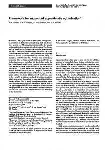
Fig. 2. Runtime (in seconds) at the central node and average runtime (in seconds) for the local optimizations, for different overlaps of features (100%: all features are available at each local node) and different numbers of nodes, correlation ratio fixed at r = 0.25. All values are averages over 20 runs with random splits of the features and approximations of ϕ.

In Figure 1, we show the test error rates for different overlaps of attributes, numbers of nodes, and correlation ratio r (averaged values over 20 repetitions

Separable Optimization of SVMs for Distributed Sensing

13

using randomized splits of features). In each plot, for a fixed number of nodes, say n = 8, we can check that the error rate increases as the correlation ratio increases. This is something expected, since as more features are correlated, more information among them can be lost by partitioning features into n groups. For a fixed correlation ratio, say 0.5 (the midpoints of four plots of Figure 1), the error rate tends to increase with the number of nodes. This will be due to the loss of information by partitioning. But it seems that such loss could be compensated by providing nodes some “overlapping” features from other nodes, which can be observed as we scan through the top left, top right, bottom left, and bottom right plots, for 32 nodes with correlation ratio r = 0.5 for instance. Scalability using multiple nodes Figure 2 shows the average runtime (in seconds) taken in the local and the central optimization of our algorithm. Since the runtime values are not affected much by the correlation ratio r, we show only the plots for r = 0.25 here. The runtime for the local optimization is keep improving until as we use more nodes up to n = 16, since all optimizations can be done in parallel (the machine had 32 physical cores). Considering the test error rates reported in the corresponding plots (top left and bottom right) in Figure 1, at correlation ratio r = 0.25, using more nodes would not harm too much the prediction performance. An exception will be n = 32, which seems to make each group too small, deteriorating both scalability and accuracy by a noticeable amount. The runtime for central optimization was almost negligible. Comparing the runtime for no and 60% overlap, the ones with overlap are slightly higher. The reason is that in the case of overlap, the number of attributes and therefore the amount of data is larger at the local nodes. 5.3

Benchmark on Real-World Data Sets

For benchmark we fix the number of nodes to 8, since it has showed a good accuracy and speed tradeoff in the experiments with our artificial data. In local optimization, we set the number of SGD iterations to 10m, ten times of the number of training examples. We compare several different implementations built upon the ASSET code: – Separated: implements Algorithm 1. – Composite: the standard SVM with approximate feature mappings corresponding to a composite kernel (2) consisting of local kernels. µj = n1 is fixed for all j = 1, 2, . . . , n. – Single: the standard SVM with approximate feature mappings to a single global kernel that uses all features. All of these make use of approximations to the kernel feature mappings. We also use SVMLight with its default parameters to make comparisons to the cases using exact kernel information.

14

S. Lee, M. Stolpe and K. Morik

Table 4. Training CPU time (in seconds, h:hours) and test error rate (mean and standard deviation %) in parentheses. The features of input vectors are distributed in two different ways: (i) each node contains disjoint set of features (no overlap), or (ii) has 25% of its features as copies from other nodes (25% overlap). ASSET-SVM Separated Composite + Central − Central ADULT 28(20.0±0.02) 9(20.6±1.17) 44(15.5±0.64) MNIST 101(11.1±0.39) 87(11.1±0.39) 539 ( 7.0±0.72) CCAT 4475(26.3±1.00) 4463(26.3±1.00) 8h(20.9±0.63) IJCNN 67 ( 9.1±0.88) 20 ( 9.5±0.07) 86 ( 4.1±0.53) COVTYPE 234(29.3±2.76) 82(35.2±1.05) 373(21.1±0.61) No Overlap

ASSET-SVM Separated Composite + Central − Central ADULT 28(19.0±1.69) 9(19.7±1.34) 48(15.5±0.49) MNIST 112(11.1±0.39) 94(12.1±0.72) 486 ( 7.3±0.50) CCAT 5779(29.5±1.01) 5768(29.5±1.01) 10h(23.8±0.80) IJCNN 75 ( 8.6±1.05) 20 ( 9.4±0.63) 107 ( 3.8±0.56) COVTYPE 219(29.6±2.76) 94(33.7±1.34) 466(20.8±0.63) 25% Overlap

Single

SVMLight

235(15.7±0.74) 966(15.1) 1539 ( 7.0±0.45) 1031 (1.1) 5656 (4.2) 177 ( 1.6±0.13) 687 (0.7) 938(18.0±0.78) 23h (7.4) Single

SVMLight

235(15.7±0.74) 966(15.1) 1539 ( 7.1±0.45) 1031 (1.1) 5656 (4.2) 177 ( 1.6±0.13) 687 (0.7) 938(18.0±0.78) 23h (7.4)

Table 4 shows the runtime and test error rate values over 20 repeated runs, except for CCAT where we use 12 runs due to its long runtime, of all methods for the five benchmark data sets, without and with 25% overlap of the features. In each run we randomize the partitioning of features and the projections for constructing approximate feature mappings, if applicable. For Single ASSET, the overlap parameter has no effect, so the results are copied in both tables for readability. The results for Single on CCAT are unavailable since its unreasonably long runtime. Gap due to the separation of optimization We first compare Separated and Composite. The difference here occurs because of our construction of the separable surrogate objective function in (8). Comparing to the third column (Composite) of Table 4, the test error rates in the second column (Separated without central optimization) has been increased by 1.63 (no overlap) and 1.65 (25% overlap) times on average. Considering that Composite has the access to all feature information, through a single composite kernel consisting of all localized kernels, such increments seem to be moderate. In Separated, features and optimizations are distributed among the nodes, and thereby the SVM can be solved in much shorter time (about 5 times faster on average) but sacrificing accuracy. Improvement by central optimization The first two columns of Table 4 show the potential improvement and cost of an additional central optimization.

Separable Optimization of SVMs for Distributed Sensing

15

The improvements in test error rates seem to be marginal (6 ∼ 7%), but recall that these are obtained using a small subsample (5000) from each training set in the central problem, rather than the entire set, simulating a low communication bound. Gap due to using localized kernels In the third and fourth columns of Table 4, the information of all features is accessed through a composite kernel consisting of local kernels (Composite), and through a single kernel using all features directly (Single). The Composite approach is very similar to the standard MKL, although we are using fixed weights among the local kernels. As we can see, the performance in terms of error rates is not very different in these two approaches. The runtime of Composite has been shorter than Single, although they have essentially the same time complexity. The savings in Composite come from the fact that the input vectors are sparse in our benchmark sets, where subvectors of them tend to be more sparse, reducing the time for projections on random directions in constructing approximate feature mappings. Gap due to approximating kernels The difference in the last two columns of Table 4 is resulted from the fact that the feature mappings of kernels are approximated in Single, whereas SVMLight uses exact kernels. The error rates of Single are comparable in most cases, except for CCAT and COVTYPE. We believe the results will improve by using different types of approximation for CCAT, and using more number of iterations in local optimization for COVTYPE. We refer to [16, 11] for more extensive comparison in this respect.

6

Conclusion

We suggest a separable optimization framework for solving the support vector machines on distributed sensor measurements, minimizing communication cost to construct a global predictor. While sacrificing some accuracy, our algorithm can run in sensor networks, providing an upper bounding estimate of error rate. Acknowledgements The authors acknowledge the support of Deutsche Forschungsgemeinschaft (DFG) within the Collaborative Research Center SFB 876 “Providing Information by Resource-Constrained Analysis”, project B3 and C1.

References 1. Bach, F.R., Lanckriet, G.R.G., Jordan, M.I.: Multiple kernel learning, conic duality, and the SMO algorithm. In: Proceedings of the 21st International Conference on Machine Learning (2004)

16

S. Lee, M. Stolpe and K. Morik

2. Bi, J., Zhang, T., Bennett, K.P.: Column-generation boosting methods for mixture of kernels. In: Proceedings of the 10th ACM SIGKDD international conference on Knowledge discovery and data mining. pp. 521–526 (2004) 3. Drineas, P., Mahoney, M.W.: On the nystrom method for approximating a gram matrix for improved kernel-based learning. Journal of Machine Learning Research 6, 2153–2175 (2005) 4. Fine, S., Scheinberg, K.: Efficient svm training using low-rank kernel representations. Journal of Machine Learning Research 2, 243–164 (2001) 5. Hastie, T., Tibshirani, R., Friedman, J.H.: The Elements of Statistical Learning. Springer (2001) 6. Joachims, T., Finley, T., Yu, C.N.: Cutting-plane training of structural svms. Machine Learning 77(1), 27–59 (2009) 7. Joachims, T.: Making large-scale support vector machine learning practical. In: Sch¨ olkopf, B., Burges, C., Smola, A. (eds.) Advances in Kernel Methods - Support Vector Learning, chap. 11, pp. 169–184. MIT Press, Cambridge, MA (1999) 8. Kloft, M., Brefeld, U., Sonnenburg, S., Zien, A.: !p -norm multiple kernel learning. Journal of Machine Learning Research 12, 953–997 (2011) 9. Lanckriet, G.R.G., De Bie, T., Cristianini, N., Jordan, M.I., Noble, W.S.: A statistical framework for genomic data fusion. Bioinformatics 20(16), 2626–2635 (2004) 10. Lanckriet, G., Cristianini, N., Bartlett, P., E.G., L., Jordan, M.: Learning the kernel matrix with semidefinite programming. In: Proceedings of the 19th International Conference on Machine Learning (2002) 11. Lee, S., Wright, S.J.: ASSET: Approximate stochastic subgradient estimation training for support vector machines. In: International Conference on Pattern Recognition Applications and Methods (2012) 12. Lippi, M., Bertini, M., Frasconi, P.: Collective traffic forecasting. In: Proceedings of the 2010 European conference on Machine learning and knowledge discovery in databases: Part II. pp. 259–273 (2010) 13. Morik, K., Bhaduri, K., Kargupta, H.: Introduction to data mining for sustainability. Data Mining and Knowledge Discovery 24(2), 311–324 (2012) 14. Nemirovski, A., Juditsky, A., Lan, G., Shapiro, A.: Robust stochastic approximation approach to stochastic programming. SIAM Journal on Optimization 19(4), 1574–1609 (2009) 15. Nemirovski, A., Yudin, D.B.: Problem complexity and method efficiency in optimization. John Wiley (1983) 16. Rahimi, A., Recht, B.: Random features for large-scale kernel machines. In: Advances in Neural Information Processing Systems, vol. 20, pp. 1177–1184. MIT Press (2008) 17. Rakotomamonjy, A., Bach, F., Canu, S., Grandvalet., Y.: More efficiency in multiple kernel learning. In: Proceedings of the 24th international conference on machine learning (2007) 18. Sonnenburg, S., R¨ atsch, G., Sch¨ afer, C., Sch¨ olkopf, B.: Large scale multiple kernel learning. Journal of Machine Learning Research 7, 1531–1565 (July 2006) 19. Wahba, G.: Splines Models for Observational Data, CBMS-NSF Regional Conference Series in Applied Mathematics, vol. 59. SIAM (1990) 20. Zinkevich, M.: Online convex programming and generalized infinitesimal gradient ascent. In: Proceedings of the 20th International Conference on Machine Learning. pp. 928–936 (2003)