Separation of variables in an asymmetric cyclidic coordinate system

arXiv:1301.3559v1 [math.CA] 16 Jan 2013

Separation of variables in an asymmetric cyclidic coordinate system H S Cohl1 and H Volkmer2 1

Applied and Computational Mathematics Division, National Institute of Standards and Technology, Gaithersburg, MD 20899-8910, USA 2 Department of Mathematical Sciences, University of Wisconsin–Milwaukee, P. O. Box 413, Milwaukee, WI 53201, USA Abstract. A global analysis is presented of solutions for Laplace’s equation on threedimensional Euclidean space in one of the most general orthogonal asymmetric confocal cyclidic coordinate systems which admit solutions through separation of variables. We refer to this coordinate system as five-cyclide coordinates since the coordinate surfaces are given by two cyclides of genus zero which represent the inversion at the unit sphere of each other, a cyclide of genus one, and two disconnected cyclides of genus zero. This coordinate system is obtained by stereographic projection of sphero-conal coordinates on four-dimensional Euclidean space. The harmonics in this coordinate system are given by products of solutions of second-order Fuchsian ordinary differential equations with five elementary singularities. The Dirichlet problem for the global harmonics in this coordinate system is solved using multiparameter spectral theory in the regions bounded by the asymmetric confocal cyclidic coordinate surfaces.

PACS numbers: 41.20.Cv, 02.30.Em, 02.30.Hq, 02.30.Jr AMS classification scheme numbers: 35J05, 42C15, 34L05, 35J15, 34B30

Cyclidic coordinate system

2

1. Introduction In 1894 Maxime Bôcher’s book “Ueber die Reihenentwicklungen der Potentialtheorie” was published [2]. It took its origin from lectures given by Felix Klein in Göttingen (see for instance [7, 8]). In Bôcher’s book, the author gives a list of 17 inequivalent coordinate systems in three dimensions in which the Laplace equation admits separated solutions of the form U (x, y, z) = R(x, y, z)w1 (s1 )w2 (s2 )w3 (s3 ),

(1)

where the modulation factor R(x, y, z) [11, p. 519] is a known and fixed function, and s1 , s2 , s3 are curvilinear coordinates of x, y, z. The functions w1 , w2 , w3 are solutions of second order ordinary differential equations. The symmetry group of Laplace’s equation is the conformal group and equivalence between various separable coordinate systems is established by the existence of a conformal transformation which maps one separable coordinate system to another. In general, the coordinate surfaces (called confocal cyclides) are given by the zero sets of polynomials in x, y, z of degree at most 4 which can be broken up into several different subclasses. For instance, eleven of these coordinate systems have coordinate surfaces which are given by confocal quadrics [9, Systems 1–11 on p. 164], nine are rotationally-invariant [9, Systems 2,5–8 on p. 164 and 14–17 on p. 210], four are cylindrical [9, Systems 1–4], and five which are the most general, are of the asymmetric type namely, confocal ellipsoidal, paraboloidal, sphero-conal, and two cyclidic coordinate systems [9, Systems 9,10,11 on p. 164 and Systems 12,13 on p. 210]). Bôcher [2] showed how to solve the Dirichlet problem for harmonic functions on regions bounded by such confocal cyclides. However, it is stated repeatedly in Bôcher’s book that the presentation lacked convergence proofs, for instance, this is mentioned in the preface written by Felix Klein. It is the purpose of this paper to supply the missing proofs for one of the asymmetric cyclidic coordinate systems which is listed as number 12 in Miller’s list [9, page 210] (see also Boyer, Kalnins & Miller (1976) [3, Table 2] and Boyer, Kalnins & Miller (1978) [4] for a more general setting). For lack of a better name we call it 5-cyclide coordinates. This asymmetric orthogonal curvilinear coordinate system has coordinates si ∈ R (i = 1, 2, 3) with si in (a0 , a1 ), (a1 , a2 ) or (a2 , a3 ), respectively where a0 < a1 < a2 < a3 are given numbers. This coordinate system is described by coordinate surfaces si = const which are five compact cyclides. The surfaces s1 = const for s1 ∈ (a0 , a1 ) are two cyclides of genus zero representing inversions at the unit sphere of each other. The surface s2 = const for s2 ∈ (a1 , a2 ) represents a ring cyclide of genus one and the surfaces s3 = const for s3 ∈ (a2 , a3 ) represent two disconnected cyclides of genus zero with reflection symmetry about the x, y-plane. The asymptotic behavior of this coordinate system as the size of these compact cyclides increases without limit is 6sphere coordinates (see Moon & Spencer (1961) [10, p. 122]), the inversion of Cartesian coordinates.


3

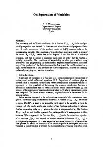
In our notation the coordinate surfaces of this system are given by the variety 4x2 4y 2 4z 2 (x2 + y 2 + z 2 − 1)2 + + + = 0, (2) s − a0 s − a1 s − a2 s − a3 where s = si is either in (a0 , a1 ), (a1 , a2 ) or (a2 , a3 ) respectively. See Figure 1(a,b) for

Figure 1. Surfaces s1,2,3 = const for ai = i, where only the component of the cyclide s1 = const inside the ball x2 + y 2 + z 2 < 1 is shown.

a graphical illustration of these triply-orthogonal coordinate surfaces, where we have selected one of the confocal cyclides for s1 = const. This is a very general coordinate system containing the parameters a0 , a1 , a2 , a3 which generates many other coordinate systems by limiting processes. Since the book by Bôcher is quite old and uses very geometrical methods, we will present our results independently of Bôcher’s book. We supply convergence proofs based on general multiparameter spectral theory [1, 13] which was created with such applications in mind. As far as we know this general theory has never before been applied to the Dirichlet problems considered by Bôcher. We start with the observation that 5-cyclide coordinates are the stereographic image of sphero-conal coordinates in four dimensions (or, expressed in another way, of ellipsoidal coordinates on the hypersphere S3 ). We take the sphero-conal coordinate system as known but we present the needed facts in Section 2. The well-known stereographic projection is dealt with in Section 3 which also explains the appearance of the factor R in (1). The 5-cyclide coordinate system is introduced in Section 4. The solution of the Dirichlet problem on regions bounded by surfaces (2) with s ∈ (a1 , a2 ) is presented in Section 6. The preceding Section 5 provides the needed convergence proofs based on multiparameter spectral theory. The remaining sections treat the Dirichlet problem on regions bounded by the surfaces (2) when s ∈ (a1 , a2 ) (ring cyclides) and s ∈ (a2 , a3 ).


4

2. Sphero-conal coordinates on Rk+1 Let k ∈ N. In order to introduce sphero-conal coordinates on Rk+1 , fix real numbers a0 < a1 < a2 < . . . < ak .

(3)

Let (x0 , x1 , . . . , xk ) be in the positive cone of Rk+1 x0 > 0, . . . , xk > 0.

(4)

Its sphero-conal coordinates r, s1 , . . . , sk are determined in the intervals r > 0, ai−1 < si < ai ,

i = 1, . . . , k

(5)

by the equations 2

r =

k X

x2j

(6)

j=0

and k X j=0

x2j = 0 for i = 1, . . . , k. s i − aj

(7)

The latter equation determines s1 , s2 , . . . , sk as the zeros of a polynomial of degree k with coefficients which are polynomials in x20 , . . . , x2k . In this way we obtain a bijective (real-)analytic map from the positive cone in Rk+1 to the set of points (r, s1 , . . . , sk ) satisfying (5). The inverse map is found by solving a linear system. It is also analytic, and it is given by Qk (si − aj ) 2 2 xj = r Qk i=1 . (8) (a − a ) i j j6=i=0 Sphero-conal coordinates are orthogonal, and its scale factors (metric coefficients) are given by Hr = 1, and Qk k 2 X x 1 1 j i6=j=1 (si − sj ) 2 Hs2i = = − r , i = 1, 2, . . . , k. (9) Q k 4 j=0 (si − aj )2 4 j=0 (si − aj ) Consider the Laplace equation ∆U =

k X ∂ 2U i=0

∂x2i

=0

(10)

for a function U (x0 , x1 , . . . , xk ). Using (9) we transform this equation to sphero-conal coordinates, and then we apply the method of separation of variables [12] U (x0 , x1 , . . . , xk ) = w0 (r)w1 (s1 )w2 (s2 ) . . . wk (sk ). For the variable r we obtain the Euler equation 4λ0 k w000 + w00 + 2 w0 = 0 r r

(11)

(12)

Cyclidic coordinate system while for each of the variables s1 , s2 , . . . , sk we obtain the Fuchsian equation " # " k−1 # k k Y X X 1 1 (s − aj ) w00 + w0 + λi sk−1−i w = 0. 2 s − a j j=0 j=0 i=0

5

(13)

More precisely, if λ0 , . . . , λk−1 are any given numbers (separation constants), and if w0 (r), r > 0, solves (12) and wi (si ), ai−1 < si < ai , solve (13) for each i = 1, . . . , k, then U defined by (11) solves (10) in the positive cone of Rk+1 (4). Equation (13) has only regular points except for k + 2 regular singular points at s = a0 , a1 , . . . , ak and s = ∞. The exponents at each finite singularity s = aj are 0 and 1 . Therefore, for each choice of parameters λ0 , . . . , λk−1 , there is a nontrivial analytic 2 solution at s = aj and another one of the form w(s) = (s−aj )1/2 v(s), where v is analytic at aj . If ν, µ denote the exponents at s = ∞ then k−1 . (14) µν = λ0 , µ + ν = 2 Pk−1 λi sk−1−i appearing in (13) is known as van Vleck polynomial. If The polynomial i=0 k = 1 then (13) is the hypergeometric differential equation (up to a linear substitution). If k = 2 then (13) is the Heun equation. We will use this equation for k = 3. According to Miller (1977) [9, p. 209] (see also [3, p. 71]) in reference to the k = 3 case, “Very little is known about the solutions.” 3. Stereographic projection We consider the stereographic projection P : S3 \ {(1, 0, 0, 0)} → R3 given by 1 P (x0 , x1 , x2 , x3 ) = (x1 , x2 , x3 ). 1 − x0 The inverse map is 1 P −1 (x, y, z) = 2 (x2 + y 2 + z 2 − 1, 2x, 2y, 2z). 2 x + y + z2 + 1 We extend P −1 to a bijective map Q : (0, ∞) × R3 → R4 \ {(x0 , 0, 0, 0) : x0 ≥ 0} by defining Q(r, x, y, z) := rP −1 (x, y, z). If we set (x0 , x1 , x2 , x3 ) = Q(r, x, y, z) we may consider r, x, y, z as curvilinear coordinates on R4 with Cartesian coordinates x0 , x1 , x2 , x3 . We note that x20 + x21 + x22 + x23 = r2 so r is just the distance between (x0 , x1 , x2 , x3 ) and the origin. Moreover, (x, y, z) is the stereographic projection of the point (x0 /r, x1 /r, x2 /r, x3 /r) ∈ S3 . It is easy to check that the coordinate system is orthogonal and scale factors are 1 hr = 1, hx = hy = hz = 2rh, where h := 2 . 2 x + y + z2 + 1


6

Let U (x0 , x1 , x2 , x3 ) = V (r, x, y, z). Then 1 ∆U = 3 3 (2rhVx )x + (2rhVy )y + (2rhVz )z + (8r3 h3 Vr )r . 8r h Suppose that U is homogeneous of degree α: U (tx0 , tx1 , tx2 , tx3 ) = tα U (x0 , x1 , x2 , x3 ),

(15)

t > 0.

Then V can be written in the form V (r, x, y, z) = rα w(x, y, z), and (15) implies rα−2 (hwx )x + (hwy )y + (hwz )z + 4α(α + 2)h3 w . 3 4h We now introduce the function ∆U =

(16)

u(x, y, z) = w(x, y, z)(x2 + y 2 + z 2 + 1)−1/2 . Then a direct calculation changes (16) to rα−2 2 u + u + u + (3 + 4α(α + 2))h u . (17) xx yy zz 4h5/2 If 3 + 4α(α + 2) = 0 then U is harmonic if and only if u is harmonic. Noting that 3 + 4α(α + 2) = (2α + 1)(2α + 3), we obtain the following theorem. ∆U =

Theorem 3.1. Let D be an open subset of S3 not containing (1, 0, 0, 0), let E = {(rx0 , rx1 , rx2 , rx3 ) : r > 0, (x0 , x1 , x2 , x3 ) ∈ D}, and let F = P (D) be the stereographic image of D. Let the function U : E → R be homogeneous of degree − 21 or − 32 , and let w : F → R satisfy U = w ◦ P on D. Then U is harmonic on E if and only if w(x, y, z)(x2 + y 2 + z 2 + 1)−1/2 is harmonic on F . 4. Five-cyclide coordinate system on R3 We introduce sphero-conal coordinates r > 0,

a0 < s1 < a1 < s2 < a2 < s3 < a3 ,

on R4 as explained in Section 2 with k = 3. Then s1 , s2 , s3 form a coordinate system for the intersection of the hypersphere S3 with the positive cone in R4 . Using the stereographic projection P from Section 3 we project these coordinates to R3 . We obtain a coordinate system for the set T = {(x, y, z) : x, y, z > 0, x2 + y 2 + z 2 > 1}.

(18)

Explicitly, x=

x1 , 1 − x0

y=

x2 , 1 − x0

z=

x3 , 1 − x0

(19)

where x2j

Q3 (si − aj ) = Q3 i=1 , j6=i=0 (ai − aj )

j = 0, 1, 2, 3.

(20)


7

Conversely, the coordinates s1 , s2 , s3 of a point (x, y, z) ∈ T are the solutions of 4x2 4y 2 4z 2 (x2 + y 2 + z 2 − 1)2 + + + = 0. (21) s − a0 s − a1 s − a2 s − a3 Since sphero-conal coordinates are orthogonal and the stereographic projection preserves angles, 5-cyclide coordinates are orthogonal, too. This is the twelfth coordinate system in Miller (1977) [9, page 210]. Miller uses a slightly different notation: a0 = 0, a1 = 1, a2 = b, a3 = a, and s1 = ρ, s2 = ν, s3 = µ. Also, x, z are interchanged. In order to calculate the scale factors for the 5-cyclide coordinate system we proceed as follows. We start with 1 ∂x1 x1 ∂x0 ∂x = + , ∂si 1 − x0 ∂si (1 − x0 )2 ∂si and similar formulas for the derivatives of y and z. Then using ∂x1 ∂x2 ∂x3 ∂x0 x20 + x21 + x22 + x23 = 1, x0 + x1 + x2 + x3 =0 ∂si ∂si ∂si ∂si a short calculation gives 3 X ∂x` ∂x` ∂x ∂x ∂y ∂y ∂z ∂z 1 + + = . ∂si ∂sj ∂si ∂sj ∂si ∂sj (1 − x0 )2 `=0 ∂si ∂sj

This confirms that 5-cyclide coordinates are orthogonal and from (9) we obtain the squares of their scale factors 1 (ρ2 − 1)2 4x2 4y 2 4z 2 2 hi = + + + , (22) 16 (si − a0 )2 (si − a1 )2 (si − a2 )2 (si − a3 )2 where ρ2 = x2 + y 2 + z 2 , or, equivalently, (s3 − s1 )(s2 − s1 ) 1 2 (ρ + 1)2 , 16 (s1 − a0 )(a1 − s1 )(a2 − s1 )(a3 − s1 ) 1 (s2 − s1 )(s3 − s2 ) , h22 = (ρ2 + 1)2 16 (s2 − a0 )(s2 − a1 )(a2 − s2 )(a3 − s2 ) 1 (s3 − s1 )(s3 − s2 ) h23 = (ρ2 + 1)2 . 16 (s3 − a0 )(s3 − a1 )(s3 − a2 )(a3 − s3 )

h21 =

(23) (24) (25)

We find harmonic functions by separation of variables in 5-cyclide coordinates as follows. Theorem 4.1. Let w1 : (a0 , a1 ) → C, w2 : (a1 , a2 ) → C, w3 : (a2 , a3 ) → C be solutions of the Fuchsian equation " # 3 3 Y X 1 1 3 2 00 0 (s − aj ) w + w + s + λ1 s + λ2 w = 0, (26) 2 s − a 16 j j=0 j=0 where λ1 , λ2 are given (separation) constants. Then the function u(x, y, z) = (x2 + y 2 + z 2 + 1)−1/2 w1 (s1 )w2 (s2 )w3 (s3 ) is a harmonic function on the set (18).

(27)


8

Proof. Using sphero-conal coordinates r, s1 , s2 , s3 on R4 , we define a function U in the positive cone of R4 by U (x0 , x1 , x2 , x3 ) = r−1/2 w1 (s1 )w2 (s2 )w3 (s3 ). 3 . The results from Section 2 The function r−1/2 is a solution of (12) when k = 3, λ0 = 16 imply that U is harmonic, and, of course, U is homogeneous of degree − 12 . The function w defined on the set (18) by U = w ◦ P is given in 5-cyclide coordinates by

w(x, y, z) = w1 (s1 )w2 (s2 )w3 (s3 ). Therefore, Theorem 3.1 gives the statement of the theorem. Equation (26) has five regular singularities at s = a0 , a1 , a2 , a3 , ∞. The exponents at the finite singularities are 0 and 21 . Using (14), we find that the exponents at infinity are 41 and 34 . So all five singularities are elementary in the sense of Ince [5]. Equation (26) is one of the standard equations in the classification of Ince [5, page 500]. We define the 5-cyclide coordinates s1 , s2 , s3 for an arbitrary point (x, y, z) ∈ R3 as the zeros s1 ≤ s2 ≤ s3 of the cubic equation 2 3 Y 4x2 4y 2 4z 2 (x + y 2 + z 2 − 1)2 + + + (s − aj ) = 0. (28) s − a s − a s − a s − a 0 1 2 3 j=0 For example, sj (0, 0, 0) = aj for j = 1, 2, 3. Each function sj : R3 → [aj−1 , aj ] is continuous. We observe that, in general, there are 16 different points in R3 which have the same coordinates s1 , s2 , s3 . If (x, y, z) is one of these points the other ones are obtained by applying the group generated by inversion at S2 σ0 (x, y, z) = ρ−2 (x, y, z)

(29)

and reflections at the coordinate planes σ1 (x, y, z) = (−x, y, z), σ2 (x, y, z) = (x, −y, z), σ3 (x, y, z) = (x, y, −z).(30) It is of interest to determine the sets where sj = aj−1 or sj = aj . We obtain s1 = a0 iff x2 + y 2 + z 2 = 1, (ρ2 − 1)2 s1 = a1 iff x = 0 and a1 − a0 (ρ2 − 1)2 s2 = a1 iff x = 0 and a1 − a0 (ρ2 − 1)2 s2 = a2 iff y = 0 and a2 − a0 (ρ2 − 1)2 s3 = a2 iff y = 0 and a2 − a0 s3 = a3 iff z = 0.

(31) 2

4y a1 − a2 4y 2 + a1 − a2 4x2 + a2 − a1 4x2 + a2 − a1 +

2

4z a1 − a3 4z 2 + a1 − a3 4z 2 + a2 − a3 4z 2 + a2 − a3 +

≥ 0,

(32)

≤ 0,

(33)

≥ 0,

(34)

≤ 0,

(35) (36)

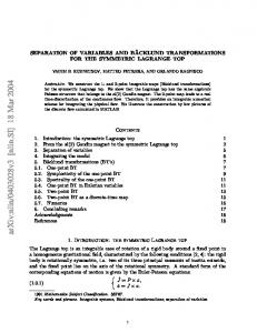
We define the sets (consisting each of two closed curves) A1 := {(x, y, z) ∈ R3 : s1 = s2 = a1 } (ρ2 − 1)2 4y 2 4z 2 = {(x, y, z) : x = 0, + + = 0}, a1 − a0 a1 − a2 a1 − a3

(37)


9

see Figure 2, and A2 := {(x, y, z) ∈ R3 : s2 = s3 = a2 } (38) 2 2 2 2 4x 4z (ρ − 1) = {(x, y, z) : y = 0, + + = 0}, a2 − a0 a2 − a1 a2 − a3 see Figure 3. Clearly, sj is analytic at all points (x, y, z) at which sj is a simple z 2

1

–2

y

0

–1

1

2

–1

–2

Figure 2. The set A1 in the y, z-plane for ai = i.

z 3

2

1

x –1

–0.5 0

0.5

1

1.5

–1

–2

–3

Figure 3. The set A2 in the x, z-plane for ai = i.


10

zero of the cubic equation (28). Therefore, s1 is analytic on R3 \ A1 , s2 is analytic on R3 \ (A1 ∪ A2 ), and s3 is analytic on R3 \ A2 . We may use (27) to define u(x, y, z) for all (x, y, z) ∈ R3 . Since the solutions w1 , w2 , w3 of (26) have limits at the end points of their intervals of definition (because the exponents are 0 and 21 there), we see that u is a continuous functions on R3 . The function (x2 + y 2 + z 2 + 1)1/2 u(x, y, z) is invariant under σi , i = 0, 1, 2, 3. In general, u is harmonic only away from the coordinate planes and the unit sphere. In fact, we observe that u is a bounded function which converges to 0 at infinity, so, by Liouville’s theorem, u cannot be harmonic on all of R3 unless it is identically zero. 5. First two-parameter Sturm-Liouville problem We consider equation (26) on the intervals (a1 , a2 ) and (a2 , a3 ) and write it in formally self-adjoint form. Setting ω(s) := |(s − a0 )(s − a1 )(s − a2 )(s − a3 )|1/2 , we obtain two Sturm-Liouville equations involving two parameters 3 2 1 0 0 s + λ1 s2 + λ2 w2 = 0, a1 < s2 < a2 , (ω(s2 )w2 ) + ω(s2 ) 16 2 3 2 1 0 0 s + λ1 s3 + λ2 w3 = 0, a2 < s3 < a3 . (ω(s3 )w3 ) − ω(s3 ) 16 3

(39)

(40) (41)

In (40) w2 is a function of s2 and the derivatives are taken with respect to s2 . In (41) w3 is a function of s3 and the derivatives are taken with respect to s3 . We simplify the equations by substituting tj = Ω(sj ), uj (tj ) = wj (sj ), where Ω(s) is the elliptic integral (see for instance [8]) Z s dσ Ω(s) := . (42) a0 ω(σ) This is an increasing absolutely continuous function Ω : [a0 , a3 ] → [0, b3 ], where bj := Ω(aj ). Let φ : [0, b3 ] → [a0 , a3 ] be the inverse function of Ω. Then (40), (41) become 3 2 00 {φ(t2 )} + λ1 φ(t2 ) + λ2 u2 = 0, b1 ≤ t2 ≤ b2 , (43) u2 + 16 3 00 2 u3 − {φ(t3 )} + λ1 φ(t3 ) + λ2 u3 = 0, b2 ≤ t3 ≤ b3 . (44) 16 We add the boundary conditions u02 (b1 ) = u02 (b2 ) = u03 (b2 ) = u03 (b3 ) = 0.

(45)

Differential equations (43), (44) together with boundary conditions (45) pose a twoparameter Sturm-Liouville eigenvalue problem. For the theory of such multiparameter problems we refer to the books [1, 13] and the references therein. A pair (λ1 , λ2 ) is called


11

an eigenvalue if there exist (nontrivial) eigenfunctions u2 (t2 ) and u3 (t3 ) which satisfy (43), (44), (45). The two-parameter problem is right-definite in the sense that φ(t ) 1 2 = φ(t3 ) − φ(t2 ) > 0 for b1 < t2 < b2 < t3 < b3 . −φ(t3 ) −1 However, this determinant is not positive on the closed rectangle [b1 , b2 ] × [b2 , b3 ]. This lack of uniform right-definiteness make some proofs in this section a little longer than they would be otherwise. We have the following Klein oscillation theorem; see [1, Theorem 5.5.1]. Theorem 5.1. For every n = (n2 , n3 ) ∈ N20 , there exists a uniquely determined eigenvalue (λ1,n , λ2,n ) ∈ R2 admitting an eigenfunction u2 with exactly n2 zeros in (b1 , b2 ) and an eigenfunction u3 with exactly n3 zeros in (b2 , b3 ). We state a result on the distribution of eigenvalues; compare with [1, Chapter 8]. Theorem 5.2. There are positive constants A1 , A2 , A3 , A4 such that, for all n ∈ N20 , − A1 (n22 + n23 + 1) ≤ λ1,n ≤ −A2 (n22 + n23 ) + A3 , |λ2,n | ≤

A4 (n22

+

n23

+ 1).

(46) (47)

Proof. If a differential equation u00 + q(t)u = 0 with continuous q : [a, b] → R admits a solution u satisfying u0 (a) = u0 (b) = 0 and having exactly m zeros in (a, b), then there π 2 m2 is t ∈ (a, b) such that q(t) = (b−a) 2 . This is shown by comparing with the eigenvalue 00 0 0 problem u + λu = 0, u (a) = u (b) = 0. Applying this fact, we find t2 ∈ (b1 , b2 ) and t3 ∈ (b2 , b3 ) such that 3 π 2 n22 2 {φ(t2 )} + λ1 φ(t2 ) + λ2 = , 16 (b2 − b1 )2 3 π 2 n23 {φ(t3 )}2 + λ1 φ(t3 ) + λ2 = − , 16 (b3 − b2 )2

(48) (49)

where we abbreviated λj = λj,n . By subtracting (48) from (49), we obtain 3 π 2 n22 π 2 n23 {φ(t3 )}2 − {φ(t2 )}2 + λ1 (φ(t3 ) − φ(t2 )) = − − ≤ 0. 16 (b2 − b1 )2 (b3 − b2 )2 Dividing by φ(t3 ) − φ(t2 ) and using 0 < φ(t3 ) − φ(t2 ) ≤ a3 − a1 , we obtain the second inequality in (46). To prove the first inequality in (46), suppose that λ1 < − 38 a3 . Then the van Vleck polynomial 3 Q(s) := s2 + λ1 s + λ2 (50) 16 satisfies Q0 (s) = 83 s + λ1 < 0 for s ≤ a3 . Let c ∈ (b1 , b2 ) be determined by φ(c) = 12 (a1 + a2 ). If Q(a2 ) ≥ 0 then, for t ∈ [b1 , c], 1 1 3 Q(φ(t)) ≥ Q( (a1 + a2 )) ≥ (a2 − a1 ) −λ1 − a3 . 2 2 8


12

By Sturm’s comparison theorem applied to equation (43), we get 3 2 (c − b1 ) (a2 − a1 ) −λ1 − a3 ≤ 4π 2 (n2 + 1)2 , 8 which gives the desired inequality. If Q(a2 ) < 0 we argue similarly working with (44) instead. Finally, (47) follows from (46) and (48). Let u2,n and u3,n denote real-valued eigenfunctions corresponding to the eigenvalue (λ1,n , λ2,n ). It is known [1, section 3.5] (and easy to prove) that the system of products u2,n (t2 )u3,n (t3 ), n ∈ N20 , is orthogonal in the Hilbert space H1 consisting of measurable functions f : (b1 , b2 ) × (b2 , b3 ) → C satisfying Z b3 Z b2 (φ(t3 ) − φ(t2 )) |f (t2 , t3 )|2 dt2 dt3 < ∞ b2

b1

with inner product Z b3 Z

b2

(φ(t3 ) − φ(t2 ))f (t2 , t3 )g(t2 , t3 ) dt2 dt3 . b2

b1

We normalize the eigenfunctions so that Z b3 Z b2 (φ(t3 ) − φ(t2 )) {u2,n (t2 )}2 {u3,n (t3 )}2 dt2 dt3 = 1. b2

(51)

b1

We have the following completeness theorem; see [13, Theorem 6.8.3]. Theorem 5.3. The double sequence of functions u2,n (t2 )u3,n (t3 ),

n ∈ N20 ,

forms an orthonormal basis in the Hilbert space H1 . The normalization (51) leads to a bound on the values of eigenfunctions. Theorem 5.4. There is a constant B > 0 such that, for all n ∈ N20 and all t2 ∈ [b1 , b2 ], t3 ∈ [b2 , b3 ], |u2,n (t2 )u3,n (t3 )| ≤ B(n22 + n23 + 1). Proof. We abbreviate uj = uj,n , λj = λj,n . Condition (51) is a normalization for the product u2 (t2 )u3 (t3 ) but not for each factor separately, so we may assume that, additionally, Z b2 {u2 (t2 )}2 dt = 1. (52) b1

Now (51), (52) imply that Z b3 (φ(t3 ) − φ(b2 )) {u3 (t3 )}2 dt3 ≤ 1. b2

(53)


13

We multiply equations (43), (44) by u2 and u3 , respectively, and integrate by parts to obtain Z b2 Z b2 Z b2 Z b2 3 2 02 2 2 (54) u22 , φu2 + λ2 u2 = φ u 2 + λ1 16 b1 b1 b1 b1 Z b3 Z b3 Z b3 Z b3 3 02 2 2 2 u3 = − u23 . (55) φu3 − λ2 φ u3 − λ1 16 b2 b2 b2 b2 It follows from (52), (54) and Theorem 5.2 that there is a constant B1 > 0 such that, for all n ∈ N20 , Z b2 2 2 u02 (56) 2 ≤ B1 (n2 + n3 + 1). b1

Unfortunately, we cannot argue the same way for u3 because we do not have an upper Rb R R bound for b23 u23 . Instead, we multiply (54) by u23 and (55) by u22 and add the equations. Then, noting (51), we find Z b2 Z b3 Z b2 Z b3 3 02 2 u2 u3 + u22 max |φ(t)|. u02 3 ≤ −λ1 + 8 t∈[b1 ,b3 ] b1 b2 b1 b2 Using Theorem 5.2 and (52), we find a constant B2 > 0 such that, for all n ∈ N20 , Z b3 2 2 (57) u02 3 ≤ B2 (n2 + n3 + 1). b2

We apply the following Lemma 5.5 (noting (52), (53), (56), (57)) and obtain the desired result. Lemma 5.5. Let u : [a, b] → R be a continuously differentiable function, and let a ≤ c < d ≤ b. Then, for all t ∈ [a, b], Z b Z d 2 2 2 |u0 (r)| dr. |u(r)| dr + 2(b − a)(d − c) (d − c) |u(t)| ≤ 2 c

a

Proof. For s, t ∈ [a, b] we have Z t Z b 1/2 2 0 1/2 0 |u(t) − u(s)| = u (r) dr ≤ |t − s| |u (r)| dr . s

a

This implies 2

2

Z

|u(t)| ≤ 2|u(s)| + 2|t − s|

b

2

|u0 (r)| dr.

a

We integrate from s = c to s = d and obtain the desired inequality. Let u1,n be the solution of 3 00 2 u1 − {φ(t1 )} + λ1,n φ(t1 ) + λ2,n u1 = 0, 16 determined by the initial conditions u1 (b1 ) = 1,

u01 (b1 ) = 0.

The following estimate on u1,n will be useful in Section 6.

b0 ≤ t1 ≤ b1 ,

(58)


14

Theorem 5.6. We have u1,n (t1 ) > 0 for all t1 ∈ [b0 , b1 ]. If 0 = b0 ≤ c1 < c2 < b1 , then there are constants C > 0 and 0 < r < 1 such that, for all n ∈ N20 and t1 ∈ [c2 , b1 ], u1,n (t1 ) ≤ Crn2 +n3 . u1,n (c1 ) Proof. We abbreviate u1 = u1,n and λj = λj,n . By definition, u1 satisfies the differential equation u001 = Q(φ(t1 ))u1 ,

t1 ∈ [b0 , b1 ],

where Q is given by (50). According to (48), (49), there are s2 ∈ (a1 , a2 ) and s3 ∈ (a2 , a3 ) such that π 2 n22 π 2 n23 Q(s2 ) = , Q(s ) = − . 3 (b2 − b1 )2 (b3 − b2 )2 If s ≤ s2 then Q(s) ≥ L(s), where L(s) is the linear function with L(sj ) = Q(sj ), j = 2, 3. It follows that Q(s) ≥ 0 for s ∈ [a0 , a1 ] and Q(φ(t1 )) ≥ C1 (n2 + n3 )2

for t1 ∈ [b0 , c2 ],

(59)

where C1 is a positive constant independent of n. We now apply the following Lemma 5.7 to complete the proof. Note that the interval [a, b] in the lemma is [c1 , b1 ] but with the end points interchanged. Lemma 5.7. Let u : [a, b] → R be a solution of the differential equation u00 (t) = q(t)u(t),

t ∈ [a, b],

determined by the initial conditions u(a) = 1, u0 (a) = 0, where q : [a, b] → R is a continuous function. Suppose that q(t) ≥ 0 on [a, b] and q(t) ≥ λ2 on [c, b] for some λ > 0 and c ∈ [a, b). Then u(t) > 0 for all t ∈ [a, b], and u(b) 1 ≥ eλ(b−c) for all t ∈ [0, c]. u(t) 2 Proof. Since q(t) ≥ 0, u(t) > 0 and u0 (t) ≥ 0 for t ∈ [a, b]. The function z = u0 /u satisfies the Riccati equation z 0 + z 2 = q(t), and the initial condition z(a) = 0. It follows that z(t) ≥ λ tanh(λ(t − c))

for t ∈ [c, b].

Integrating from t = c to t = b gives ln

u(b) 1 ≥ ln cosh λ(b − c) ≥ ln eλ(b−c) u(c) 2

which yields the claim since u is nondecreasing.


15

We now introduce a systematic notation for our eigenvalues and eigenfunctions. First of all, we note that the results of this section remain valid for other sets of boundary conditions. We will need eight sets of boundary conditions labeled by p = (p1 , p2 , p3 ) ∈ {0, 1}3 . These boundary conditions are u02 (b1 ) = 0 u02 (b2 ) = u03 (b2 ) = 0 u03 (b3 ) = 0

if p1 = 0, if p2 = 0, if p3 = 0,

u2 (b1 ) = 0 u2 (b2 ) = u3 (b2 ) = 0 u3 (b3 ) = 0

if p1 = 1, if p2 = 1, (60) if p3 = 1.

The initial conditions for u1 are u1 (b1 ) = 1, u01 (b1 ) = 0 if p1 = 0,

u1 (b1 ) = 0, u01 (b1 ) = 1 if p1 = 1. (61) (1)

(1)

We denote the corresponding eigenvalues by (λ1,n,p , λ2,n,p ). For the notation of eigenfunctions we return to the si -variable connected to ti by ti = Ω(si ). The (1) eigenfunctions will be denoted by Ei,n,p (si ) = ui,n (ti ), i = 1, 2, 3. The superscript (1) is used to distinguish from eigenvalues and eigenfunctions introduced in Sections 7 (1) (1) and 9. The subscript n = (n2 , n3 ) indicates the number of zeros of E2,n,p (s2 ), E3,n,p (s3 ) in (a1 , a2 ), (a2 , a3 ), respectively. The subscript p indicates the boundary conditions used to determine eigenvalues and eigenfunctions. By using the letter E for eigenfunctions we follow Bôcher [2]. In our notation we suppressed the dependence of eigenvalues and eigenfunctions on a0 , a1 , a2 , a3 . (1) Summarizing, for i = 1, 2, 3, Ei,n,p is a solution of (26) on (ai−1 , ai ) with (λ1 , λ2 ) = (1) (2) (1) (λ1,n,p , λ2,n,p ). The solution E1,n,p (s1 ) has exponent 12 p1 at a1 and it has no zeros in (1) (a0 , a1 ). The solution E2,n,p (s2 ) has exponent 12 p1 at a1 , exponent 12 p2 at a2 , and its has (1) n2 zeros in (a1 , a2 ). The solution E3,n,p (s3 ) has exponent 21 p2 at a2 , exponent 21 p3 at a3 , and it has n3 zeros in (a2 , a3 ). 6. First Dirichlet problem Consider the coordinate surface (21) for fixed s = d1 ∈ (a0 , a1 ). See Figure 4 for a graphical depiction of the shape of this surface. Let (x0 , y 0 , z 0 ) ∈ S2 . The ray (x, y, z) = t(x0 , y 0 , z 0 ), t > 0, intersects the surface if (t2 − 1)2 = ct2 , d 1 − a0

(62)

where 4x02 4y 02 4z 02 + + > 0. a1 − d 1 a2 − d 1 a3 − d 1 Equation (62) has two positive solutions t = t1 , t2 such that 0 < t1 < 1 < t2 and t1 t2 = 1. Therefore, the coordinate surface s1 = d1 consists of two disjoint closed surfaces of genus 0. One lies inside the unit ball B1 (0) centered at the origin and the other one is the image of it under the inversion (29). Let D1 be the region interior to the first surface, that is, c=

D1 = {(x, y, z) ∈ B1 (0) : s1 > d1 },

(63)


16

Figure 4. Coordinate surfaces s1 = const for ai = i with (a), (b) inside B1 (0), (d), (e), (f) outside B1 (0), and (c) the unit sphere.

or, equivalently, (ρ2 − 1)2 4x2 4y 2 4z 2 + + + > 0}. d 1 − a0 d 1 − a1 d 1 − a2 d 1 − a3 We showed that D1 is star-shaped with respect to the origin. We now solve the Dirichlet problem for harmonic functions in D1 by the method of separation of variables. (1) Let p = (p1 , p2 , p3 ) ∈ {0, 1}3 and n = (n2 , n3 ) ∈ N20 . Using the functions Ei,n,p introduced in Section 5 we define the internal 5-cyclidic harmonic of the first kind D1 = {(x, y, z) ∈ B1 (0) :

(1)

(1)

(1)

2 2 2 −1/2 G(1) E1,n,p (s1 )E2,n,p (s2 )E3,n,p (s3 ) n,p (x, y, z) = (x + y + z + 1)

(64)

for x, y, z ∈ B1 (0) with x, y, z ≥ 0. We extend this function to B1 (0) as a function of parity p. We call a function f of parity p if f (σi (x, y, z)) = (−1)pi f (x, y, z),

for i = 1, 2, 3

(65)

using the reflections (30). (1)

Lemma 6.1. The function Gn,p is harmonic on B1 (0). (1)

Proof. By Theorem 4.1, Gn,p is harmonic on B1 (0) away from the coordinate planes. (1) Therefore, it is enough to show that Gn,p is analytic on B1 (0). Consider first p = (0, 0, 0). Then (64) holds on B1 (0). Since s1 6= a0 on B1 (0), (1) Gn,p is analytic on B1 (0) \ (A1 ∪ A2 ) as a composition of analytic functions. In order


17

(1)

to show that Gn,p is also analytic at the points of A1 ∪ A2 , one may refer to a classical result on “singular curves” of harmonic functions; see Kellogg (1967) [6, Theorem XIII, page 271] but we will argue more directly. Since A1 and A2 are disjoint sets, it is (1) clear that E3,n,p (s3 ) is analytic at every point in B1 (0) ∩ A1 . In order to show that (1) (1) E1,n,p (s1 )E2,n,p (s2 ) is analytic at (x0 , y 0 , z 0 ) ∈ B1 (0) ∩ A1 , we argue as follows. We (1) may assume that there is an analytic function w : (a1 , a3 ) → R such that E1,n,p (1) and E2,n,p are restrictions of this function to (a1 , a2 ) and (a2 , a3 ), respectively. Now (s1 − a1 ) + (s2 − a1 ) and (s1 − a1 )(s2 − a1 ) are analytic functions of (x, y, z) in a (1) (1) neighborhood of (x0 , y 0 , z 0 ). Lemma 6.2 implies that E1,n,p (s1 )E2,n,p (s2 ) as a function (1) of (x, y, z) is analytic at (x0 , y 0 , z 0 ). It follows that Gn,p is analytic at every point in (1) B1 (0) ∩ A1 . In the same way, we show that Gn,p is analytic at every point in B1 (0) ∩ A2 . If p = (0, 0, 1) then we introduce the function √ a3 − s3 if z ≥ 0 χ := √ − a3 − s3 otherwise. It follows from (19), (20) that χ is analytic on R3 \ A2 . Then (1)

(1)

2 2 2 −1/2 G(1) E1,n,p (s1 )E2,n,p (s2 )χ(x, y, z)w3 (s3 ) n,p (x, y, z) = (x + y + z + 1)

on B1 (0), where w3 is analytic at s3 = a3 . We then argue as above. The other parity vectors p are treated similarly. Lemma 6.2. Let f : (B )2 → C, B = {s ∈ C : |s| < }, be an analytic function which is symmetric: f (s, t) = f (t, s). Let g, h : (Bδ )3 → B be functions such that g + h and gh are analytic. Then the function f (g(x, y, z), h(x, y, z)) is analytic on (Bδ )3 . Substituting tj = Ω(sj ), j = 2, 3, the Hilbert space H1 from Section 5 transforms ˜ 1 consisting of measurable functions g : (a1 , a2 ) × (a2 , a3 ) → C to the Hilbert space H for which Z a3 Z a2 s3 − s2 2 kgk := |g(s2 , s3 )|2 ds2 ds3 < ∞. (66) a2 a1 ω(s2 )ω(s3 ) ˜ 1 and fixed p, we have the Fourier expansion By Theorem 5.3, for g ∈ H X (1) (1) g(s2 , s3 ) ∼ cn,p E2,n,p (s2 )E3,n,p (s3 ),

(67)

n

where the Fourier coefficients are given by Z a3 Z a2 s3 − s2 (1) (1) cn,p = g(s2 , s3 )E2,n,p (s2 )E3,n,p (s3 ) ds2 ds3 . a2 a1 ω(s2 )ω(s3 )

(68)

Theorem 6.3. Consider the region D1 defined by (63) for some fixed d1 ∈ (a0 , a1 ). Let e be a function defined on its boundary ∂D1 of parity p ∈ {0, 1}3 , and let g(s2 , s3 ) be the representation of f (x, y, z) := (x2 + y 2 + z 2 + 1)1/2 e(x, y, z)

(69)


18

˜ 1 and expand in 5-cyclide coordinates for (x, y, z) ∈ ∂D1 with x, y, z > 0. Suppose g ∈ H g in the series (67). Then the function u(x, y, z) given by X cn,p G(1) (70) u(x, y, z) = n,p (x, y, z) (1) E (d ) 1 1,n,p n is harmonic in D1 and assumes the values e on the boundary of D1 in the L2 -sense explained below. Proof. Let d1 < d < a1 and s1 ∈ [d, a1 ]. Using Theorems 5.4, 5.6 we estimate (1) E (s ) 1 1,n,p (1) (1) E2,n,p (s2 )E3,n,p (s3 ) ≤ |cn,p |Crn2 +n3 B(n22 + n23 + 1), cn,p (1) E1,n,p (d1 ) where the constants B, C > 0 and r ∈ (0, 1) are independent of n and s1 ∈ [d, a1 ], s2 ∈ [a1 , a2 ], s3 ∈ [a2 , a3 ]. Since cn,p is a bounded double sequence, this proves that the series in (70) is absolutely and uniformly convergent on compact subsets of D1 . Consequently, by Lemma 6.1, u(x, y, z) is harmonic in D1 . If we consider u for fixed ˜ 1 by the Parseval s1 ∈ (d1 , a1 ) and compute the norm ku − ek in the Hilbert space H equality, we obtain !2 (1) X E (s ) 1 1,n,p |cn,p |2 1 − (1) ku − ek2 ≤ . E1,n,p (d1 ) n It is easy to see that the right-hand side converges to 0 as s1 → d1 . Taking into account that e and u have the same parity, it follows that u assumes the boundary values e in this L2 -sense. If e is a function on ∂D1 without parity, we write the function f from (69) as a sum of eight functions X f= fp , p

where fp is of parity p. Then the solution of the corresponding Dirichlet problem is given by X cn,p u(x, y, z) = G(1) (71) n,p (x, y, z), (1) E (d ) 1,n,p 1 n,p where Z

a3

Z

a2

cn,p = a2

a1

s3 − s2 (1) (1) gp (s2 , s3 )E2,n,p (s2 )E3,n,p (s3 ) ds2 ds3 ω(s2 )ω(s3 )

(72)

and gp (s2 , s3 ) is the representation of fp in 5-cyclide coordinates. We may write the coefficient cn,p as an integral over the surface ∂D1 itself. The surface element is dS = h2 h3 ds2 ds3 with the scale factors h2 , h3 given in (24), (25). Using 1 ω(s1 ) h2 h3 = (x2 + y 2 + z 2 + 1) (s3 − s2 ), h1 4 ω(s2 )ω(s3 )


19

we obtain from (72) cn,p =

1

Z

(1) 2ω(d1 )E1,n,p (d1 )

∂D1

e (1) G dS, h1 n,p

(73)

where h21

1 = 16

(x2 + y 2 + z 2 − 1)2 4x2 4y 2 4z 2 + + + (d1 − a0 )2 (d1 − a1 )2 (d1 − a2 )2 (d1 − a3 )2

.

7. Second two-parameter Sturm-Liouville problem We treat the two-parameter eigenvalue problem that appears when we wish to solve the Dirichlet problem in ring cyclides. It is quite similar to the one considered in Section 5, however, there are also some interesting differences. Consider equation (26) on the intervals (a0 , a1 ) and (a2 , a3 ). We obtain two Sturm-Liouville equations involving two parameters 1 3 2 0 0 (ω(s1 )w1 ) − s + λ1 s1 + λ2 w1 = 0, a0 < s1 < a1 , (74) ω(s1 ) 16 1 3 2 1 0 0 s + λ1 s3 + λ2 w3 = 0, a2 < s3 < a3 . (ω(s3 )w3 ) − (75) ω(s3 ) 16 3 We again simplify by substituting tj = Ω(sj ), uj (tj ) = wj (sj ). Then (74), (75) become 3 2 00 {φ(t1 )} + λ1 φ(t1 ) + λ2 u1 = 0, b0 ≤ t1 ≤ b1 , u1 − (76) 16 3 2 00 {φ(t3 )} + λ1 φ(t3 ) + λ2 u3 = 0, b2 ≤ t3 ≤ b3 . (77) u3 − 16 We add boundary conditions u01 (b0 ) = u01 (b1 ) = u03 (b2 ) = u03 (b3 ) = 0.

(78)

Differential equations (76), (77) together with boundary conditions (78) pose a twoparameter Sturm-Liouville eigenvalue problem. In contrast to Section 5, we now have a uniformly right-definite problem: φ(t ) 1 1 − = φ(t3 ) − φ(t1 ) ≥ a2 − a1 > 0 for b0 ≤ t1 ≤ b1 ≤ t3 ≤ b3 . φ(t3 ) 1 We again have Klein’s oscillation theorem. Theorem 7.1. For every n = (n1 , n3 ) ∈ N20 , there exists a uniquely determined eigenvalue (λ1,n , λ2,n ) ∈ R2 admitting an eigenfunction u1 with exactly n1 zeros in (b0 , b1 ) and an eigenfunction u3 with exactly n3 zeros in (b2 , b3 ). We state a result on the distribution of eigenvalues. Theorem 7.2. There are constants A1 , A2 , A3 > 0 such that, for all n ∈ N20 , − A1 (n23 + 1) ≤ λ1,n ≤ A2 (n21 + 1),

(79)

|λ2,n | ≤ A3 (n21 + n23 + 1).

(80)


20

Proof. We abbreviate λj = λj,n . Arguing as in the proof of Theorem 5.2, there are t1 ∈ [b0 , b1 ] and t3 ∈ [b2 , b3 ] such that π 2 n21 3 {φ(t1 )}2 + λ1 φ(t1 ) + λ2 = − , 16 (b1 − b0 )2 π 2 n23 3 2 {φ(t3 )} + λ1 φ(t3 ) + λ2 = − . 16 (b3 − b2 )2

(81) (82)

By subtracting (81) from (82), we obtain 3 π 2 n21 π 2 n23 {φ(t3 )}2 − {φ(t1 )}2 + λ1 (φ(t3 ) − φ(t1 )) = − 16 (b1 − b0 )2 (b3 − b2 )2 which implies (79). Now (80) follows from (79) and (81). Let u1,n and u3,n denote eigenfunctions corresponding to the eigenvalue (λ1,n , λ2,n ). The system of products u1,n (t1 )u3,n (t3 ), n ∈ N20 , is orthogonal in the Hilbert space H2 consisting of measurable functions f : (b0 , b1 ) × (b2 , b3 ) → C satisfying Z b3 Z b1 (φ(t3 ) − φ(t1 )) |f (t1 , t3 )|2 dt1 dt3 < ∞ b2

b0

with inner product Z b3 Z

b1

(φ(t3 ) − φ(t1 ))f (t1 , t3 )g(t1 , t3 ) dt1 dt3 . b2

b0

We normalize the eigenfunctions so that Z b3 Z b1 (φ(t3 ) − φ(t1 )) {u1,n (t1 )}2 {u3,n (t3 )}2 dt1 dt3 = 1. b2

(83)

b0

We have the following completeness theorem. Theorem 7.3. The double sequence of functions u1,n (t1 )u3,n (t3 ),

n ∈ N20 ,

forms an orthonormal basis in the Hilbert space H2 . The normalization (83) leads to a bound on the values of eigenfunctions. Since we have uniform right-definiteness, the proof is simpler than the proof of Theorem 5.4. Theorem 7.4. There is a constant B > 0 such that, for all n ∈ N20 and all t1 ∈ [b0 , b1 ], t3 ∈ [b2 , b3 ], |u1,n (t1 )u3,n (t3 )| ≤ B(n21 + n23 + 1). Let u2,n be the solution of 3 2 00 {φ(t2 )} + λ1,n φ(t2 ) + λ2,n u2 = 0, u2 + 16 determined by initial conditions u2 (b1 ) = 1,

u02 (b1 ) = 0.

b1 ≤ t2 ≤ b2

(84)


21

Theorem 7.5. We have u2,n (t2 ) > 0 for all t2 ∈ [b1 , b2 ]. If b1 < c1 < c2 < b2 , then there are constants C > 0 and 0 < r < 1 such that, for all n ∈ N20 and t2 ∈ [b1 , c1 ], u2,n (t2 ) n1 +n3 . u2,n (c2 ) ≤ Cr Proof. We abbreviate u2 = u2,n and λj = λj,n . We write (84) in the form u002 + Q(φ(t2 ))u2 = 0,

t2 ∈ [b1 , b2 ],

where Q is given by (50). According to (81), (82), there are s1 ∈ (a0 , a1 ) and s3 ∈ (a2 , a3 ) such that π 2 n21 π 2 n23 Q(s1 ) = − , Q(s ) = − . 3 (b1 − b0 )2 (b3 − b2 )2 If s ∈ [s1 , s3 ], then Q(s) ≤ L(s), where L(s) is the linear function with L(sj ) = Q(sj ), j = 1, 3. It follows that Q(φ(t2 )) ≤ −C(n1 + n3 )2

for t2 ∈ [c1 , c2 ].

(85)

Again, we apply Lemma 5.7 to complete the proof. The results of this section remain valid for other boundary conditions. This time we will need sixteen sets of boundary conditions labeled by p = (p0 , p1 , p2 , p3 ) ∈ {0, 1}4 . These boundary conditions are u01 (b0 ) = 0 u01 (b1 ) = 0 u03 (b2 ) = 0 u03 (b3 ) = 0

if if if if

p0 p1 p2 p3

= 0, = 0, = 0, = 0,

u1 (b0 ) = 0 u1 (b1 ) = 0 u3 (b2 ) = 0 u3 (b3 ) = 0

if if if if

p0 p1 p2 p3

= 1, = 1, = 1, = 1.

(86)


u2 (b1 ) = 0, u02 (b1 ) = 1 if p1 = 1. (2)

(2)

(87)

We denote the corresponding eigenvalues by (λ1,n,p , λ2,n,p ). The eigenfunctions will be (2) denoted by Ei,n,p (si ) = ui,n (ti ), i = 1, 2, 3. (2) Summarizing, for i = 1, 2, 3, Ei,n,p is a solution of (26) on (ai−1 , ai ) with (λ1 , λ2 ) = (2) (2) (2) (λ1,n,p , λ2,n,p ). The solution E1,n,p (s1 ) has exponent 21 p0 at a0 , exponent 12 p1 at a1 , and (2) it has n1 zeros in (a0 , a1 ). The solution E2,n,p (s2 ) has exponent 12 p1 at a1 , and its has (2) no zeros in (a1 , a2 ). The solution E3,n,p (s3 ) has exponent 21 p2 at a2 , exponent 12 p3 at a3 , and it has n3 zeros in (a2 , a3 ).


22

Figure 5. Coordinate surfaces s2,3 = const for ai = i.

8. Second Dirichlet problem Consider the coordinate surface (21) for fixed s = d2 ∈ (a1 , a2 ). See Figure 5(a,b,c) for a graphical depiction of the shape of this surface. If (x0 , y 0 , z 0 ) ∈ S2 then the ray (x, y, z) = t(x0 , y 0 , z 0 ) , t > 0, is tangent to the surface if and only if (x0 , y 0 , z 0 ) is on the surface. If (x0 , y 0 , z 0 ) is in the elliptical cone 4x02 4y 02 4z 02 + + > 0, d2 − a1 d2 − a2 d2 − a3 then the ray does not intersect the surface. Otherwise we have two intersections t = t1 , t2 and t1 t2 = 1. It follows from these considerations that s2 = d2 describes a connected surface of genus 1. The region interior to this surface is D2 = {(x, y, z) ∈ R3 : s2 < d2 },

(88)

or, equivalently, (x2 + y 2 + z 2 − 1)2 4x2 4y 2 4z 2 + + + < 0}. d2 − a0 d2 − a1 d2 − a2 d2 − a3 In this section we solve the Dirichlet problem for harmonic functions in D2 by the method of separation of variables. (2) Let p = (p0 , p1 , p2 , p3 ) ∈ {0, 1}4 and n = (n1 , n3 ) ∈ N20 . Using the functions Ei,n,p introduced in Section 7 we define the internal 5-cyclidic harmonic of the second kind D2 = {(x, y, z) :

(2)

(2)

(2)


(89)


23

for x, y, z ∈ B1 (0) with x, y, z ≥ 0. We extend the function (x2 + y 2 + z 2 + 1)1/2 G(2) n,p (x, y, z) to R3 as a function of parity p. We call a function f of parity p = (p0 , p1 , p2 , p3 ) if f (σi (x, y, z)) = (−1)pi f (x, y, z),

for i = 0, 1, 2, 3,

(90)

using inversion (29) and reflections (30). We omit the proof of the following lemma which is similar to the proof of Lemma 6.1. (2)

Lemma 8.1. The function Gn,p is harmonic at all points (x, y, z) ∈ R3 at which s2 6= a2 ; see (34). (2)

Note that s2 < d2 < a2 in D2 . Therefore, Gn,p is harmonic in an open set containing the closure of D2 . Geometrically speaking, the set s2 = a2 consists of the part of the plane y = 0 “outside” the two closed curves in Figure 3. The ring cyclide D2 passes through the y = 0 plane inside those two closed curves. Substituting tj = Ω(sj ), j = 1, 3, the Hilbert space H2 from Section 7 transforms ˜ 2 consisting of measurable functions g : (a0 , a1 ) × (a2 , a3 ) → C to the Hilbert space H for which Z a3 Z a1 s3 − s1 2 |g(s1 , s3 )|2 ds1 ds3 < ∞. (91) kgk := ω(s )ω(s ) 1 3 a2 a0 ˜ 2 and fixed p, we have the Fourier expansion By Theorem 7.3, for g ∈ H X (2) (2) cn,p E1,n,p (s1 )E3,n,p (s3 ), g(s1 , s3 ) ∼

(92)

n

where the Fourier coefficients are given by Z a3 Z a1 s3 − s1 (2) (2) cn,p = g(s1 , s3 )E1,n,p (s1 )E3,n,p (s3 ) ds1 ds3 . ω(s )ω(s ) 1 3 a2 a0 Theorem 8.2. Consider the region D2 defined by (88) for some fixed d2 ∈ (a1 , a2 ). Let e be a function defined on its boundary ∂D2 , and set f (x, y, z) := (x2 + y 2 + z 2 + 1)1/2 e(x, y, z).

(93)

Suppose that f has parity p ∈ {0, 1}4 , and its representation g(s1 , s3 ) in 5-cyclide ˜ 2 . Expand g in the series (92). Then the function u(x, y, z) given by coordinates is in H X cn,p u(x, y, z) = G(2) (94) n,p (x, y, z) (2) E (d ) 2,n,p 2 n is harmonic in D2 and assumes the values e on the boundary of D2 in the L2 -sense explained below. Proof. The proof is similar to the proof of Theorem 6.3. It uses Theorems 7.4 and 7.5 to show that the series in (94) is absolutely and uniformly convergent on compact subsets


24

of D2 . Consequently, by Lemma 8.1, u(x, y, z) is harmonic in D2 . If we consider u for ˜ 2 , we obtain fixed s2 ∈ (a1 , d2 ) and compute the norm ku − ek in the Hilbert space H !2 (2) X E (s ) 2 2,n,p . ku − ek2 ≤ |cn,p |2 1 − (2) E2,n,p (d2 ) n The right-hand side converges to 0 as s2 → d2 . Hence u assumes the boundary values e in this L2 -sense. If f is a function without parity, we write f as a sum of sixteen functions X f= fp , p∈{0,1}4

where fp is of parity p. Then the solution of the corresponding Dirichlet problem is given by X cn,p G(2) (95) u(x, y, z) = n,p (x, y, z), (2) n,p E2,n,p (d2 ) where Z

a3

Z

a1

cn,p = a2

a0


(96)

and gp (s1 , s3 ) is the representation of fp in 5-cyclide coordinates. We may also write cn,p as a surface integral Z 1 e (2) cn,p = Gn,p dS, (97) (2) 4ω(d2 )E2,n,p (d2 ) ∂D2 h2 where h22

1 = 16

(x2 + y 2 + z 2 − 1)2 4x2 4y 2 4z 2 + + + (d2 − a0 )2 (d2 − a1 )2 (d2 − a2 )2 (d2 − a3 )2

.

9. Third two-parameter Sturm-Liouville problem If we write (26) on the intervals (a0 , a1 ) and (a1 , a2 ) in formally self-adjoint form, we obtain 1 3 2 0 0 s + λ1 s1 + λ2 w1 = 0, a0 < s1 < a1 , (98) (ω(s1 )w1 ) − ω(s1 ) 16 1 1 3 2 0 0 (ω(s2 )w2 ) + s + λ1 s2 + λ2 w2 = 0, a1 < s2 < a2 . (99) ω(s2 ) 16 2 We simplify the equations by substituting tj = Ω(sj ), uj (tj ) = wj (sj ), where Ω(s) is the elliptic integral (42). Then (98), (99) become 3 00 2 u1 − {φ(t1 )} + λ1 φ(t1 ) + λ2 u1 = 0, b0 ≤ t1 ≤ b1 , (100) 16 3 00 2 {φ(t2 )} + λ1 φ(t2 ) + λ2 u2 = 0, b1 ≤ t2 ≤ b2 . (101) u2 + 16


25

Of course, this system is very similar to the one considered in Section 5. Therefore, we will be brief in this section. For a given p = (p0 , p1 , p2 ) ∈ {0, 1}3 we consider the boundary conditions u01 (b0 ) = 0 u01 (b1 ) = u02 (b1 ) = 0 u02 (b2 ) = 0

if p0 = 0, if p1 = 0, if p2 = 0,

u1 (b0 ) = 0 u1 (b1 ) = u2 (b1 ) = 0 u2 (b2 ) = 0

if p0 = 1, if p1 = 1, (102) if p2 = 1.


u3 (b2 ) = 0, u03 (b2 ) = 1 if p2 = 1. (103) (3)

(3)

We denote the corresponding eigenvalues by (λ1,n,p , λ2,n,p ), where n = (n1 , n2 ) ∈ N20 . (3) The eigenfunctions will be denoted by Ei,n,p (si ) = ui,n (ti ), i = 1, 2, 3. (3) Summarizing, for i = 1, 2, 3, Ei,n,p is a solution of (26) on (ai−1 , ai ) with (λ1 , λ2 ) = (3) (3) (3) (λ1,n,p , λ2,n,p ). The solution E1,n,p (s1 ) has exponent 12 p0 at a0 , exponent 12 p1 at a1 , and (3) it has n1 zeros in (a0 , a1 ). The solution E2,n,p (s2 ) has exponent 12 p1 at a1 , exponent 21 p2 (3) at a2 , and it has n2 zeros in (a1 , a2 ). The solution E3,n,p (s3 ) has exponent 21 p2 at a2 , and it has no zeros in (a2 , a3 ). 10. Third Dirichlet problem Consider the coordinate surface (21) for fixed s = d3 ∈ (a2 , a3 ). See Figure 5(d,e,f) for a graphical depiction of the shape of this surface. If (x0 , y 0 , z 0 ) ∈ S2 then the ray (x, y, z) = t(x0 , y 0 , z 0 ) , t > 0, is tangent to the surface if and only if (x0 , y 0 , z 0 ) is on the surface. If (x0 , y 0 , z 0 ) is in the elliptical cone 4x02 4y 02 4z 02 + + < 0, d2 − a1 d2 − a2 d2 − a3 then the ray intersects the surface twice at t = t1 , t2 with t1 t2 = 1. Otherwise, there is no intersection. Therefore, the coordinate surface s3 = d3 consists of two disjoint closed surfaces of genus 0 separated by the plane z = 0, and they are mirror images of each other under the reflection σ3 . We consider the region inside the surface s3 = d3 with z > 0 D3 = {(x, y, z) : z > 0, s3 < d3 },

(104)

or, equivalently, (x2 + y 2 + z 2 − 1)2 4x2 4y 2 4z 2 + + + < 0}. d3 − a0 d3 − a1 d3 − a2 d3 − a3 Next, we solve the Dirichlet problem for harmonic functions in D3 by the method of separation of variables. (3) Let p = (p0 , p1 , p2 ) ∈ {0, 1}3 and n = (n1 , n2 ) ∈ N20 . Using the functions Ei,n,p introduced in Section 9 we define the internal 5-cyclidic harmonic of the third kind D3 = {(x, y, z) : z > 0,

(3)

(3)

(3)


(105)


26

for (x, y, z) ∈ B1 (0) with x, y, z ≥ 0. We extend the function (x2 + y 2 + z 2 + 1)1/2 G(3) n,p (x, y, z) to the half-space {(x, y, z) : z > 0} as a function of parity p. We call a function f of parity p = (p0 , p1 , p2 ) if f (σi (x, y, z)) = (−1)pi f (x, y, z),

for i = 0, 1, 2

(106)

using the inversion σ0 and the reflections σ1 , σ2 . As before we have the following lemma. (3)

Lemma 10.1. The function Gn,p is harmonic on {(x, y, z) : z > 0}. ˜ 3 consisting of measurable functions g : (a0 , a1 ) × We have the Hilbert space H (a1 , a2 ) → C for which Z a2 Z a1 s2 − s1 2 |g(s1 , s2 )|2 ds1 ds2 < ∞. (107) kgk := ω(s )ω(s ) 1 1 a0 a1 ˜ 3 and fixed p, we have the Fourier expansion For g ∈ H X (3) (3) g(s1 , s2 ) ∼ cn,p E1,n,p (s1 )E2,n,p (s2 ),

(108)

n

where the Fourier coefficients are given by Z a2 Z a1 s2 − s1 (3) (3) g(s1 , s2 )E1,n,p (s1 )E2,n,p (s2 ) ds1 ds2 . cn,p = a1 a0 ω(s1 )ω(s2 )

(109)

Theorem 10.2. Consider the region D3 defined by (104) for some fixed d3 ∈ (a2 , a3 ). Let e be a function defined on its boundary ∂D3 , and set f (x, y, z) := (x2 + y 2 + z 2 + 1)1/2 e(x, y, z).

(110)

Suppose that f has parity p ∈ {0, 1}3 , and its representation g(s1 , s2 ) in 5-cyclide ˜ 3 . Expand g in the series (108). Then the function u(x, y, z) given coordinates is in H by X cn,p u(x, y, z) = (111) G(3) n,p (x, y, z) (3) E (d ) 3 3,n,p n is harmonic in D3 and assumes the values e on the boundary of D3 in an L2 -sense. If f is a function without parity, we write f as a sum of eight functions X f= fp , p∈{0,1}3

where fp is of parity p. Then the solution of the corresponding Dirichlet problem is given by X cn,p (112) u(x, y, z) = G(3) n,p (x, y, z), (3) n,p E3,n,p (d3 ) where Z

a2

Z

a1

cn,p = a1

a0


(113)


27

and gp (s1 , s2 ) is the representation of fp in 5-cyclide coordinates. Alternatively, we have Z e (3) 1 (114) Gn,p dS, cn,p = (3) 2ω(d3 )E3,n,p (d3 ) ∂D3 h3 where h23

1 = 16

(x2 + y 2 + z 2 − 1)2 4x2 4y 2 4z 2 + + + (d3 − a0 )2 (d3 − a1 )2 (d3 − a2 )2 (d3 − a3 )2

.

Acknowledgements This work was conducted while H. S. Cohl was a National Research Council Research Postdoctoral Associate in the Applied and Computational Mathematics Division at the National Institute of Standards and Technology, Gaithersburg, Maryland, U.S.A. References [1] F. V. Atkinson and A. B. Mingarelli. Multiparameter eigenvalue problems. Sturm-Liouville theory. CRC Press, Boca Raton, FL, 2011. [2] M. Bˆ ocher. Ueber die Reihenentwickelungen der Potentialtheorie. B. G. Teubner, Leipzig, 1894. [3] C. P. Boyer, E. G. Kalnins, and W. Miller, Jr. Symmetry and separation of variables for the Helmholtz and Laplace equations. Nagoya Mathematical Journal, 60:35–80, 1976. [4] C. P. Boyer, E. G. Kalnins, and W. Miller, Jr. R-separable coordinates for three-dimensional complex Riemannian spaces. Transactions of the American Mathematical Society, 242:355–376, 1978. [5] E. L. Ince. Ordinary differential equations. Dover Publications, New York, 1956. [6] O. D. Kellogg. Foundations of potential theory. Reprint from the first edition of 1929. Die Grundlehren der Mathematischen Wissenschaften, Band 31. Springer-Verlag, Berlin, 1967. [7] F. Klein. Ueber Lamé’sche Functionen. Mathematische Annalen, 18(2):237–246, 1881. [8] F. Klein. Ueber Normirung der linearen Differentialgleichungen zweiter Ordnung. Mathematische Annalen, 38(1):144–152, 1891. [9] W. Miller, Jr. Symmetry and separation of variables. Addison-Wesley Publishing Co., Reading, Mass.-London-Amsterdam, 1977. With a foreword by Richard Askey, Encyclopedia of Mathematics and its Applications, Vol. 4. [10] P. Moon and D. E. Spencer. Field theory handbook, including coordinate systems, differential equations and their solutions. Springer-Verlag, Berlin, 1961. [11] P. M. Morse and H. Feshbach. Methods of theoretical physics. 2 volumes. McGraw-Hill Book Co., Inc., New York, 1953. [12] D. Schmidt and G. Wolf. A method of generating integral relations by the simultaneous separability of generalized Schr¨ odinger equations. SIAM Journal on Mathematical Analysis, 10(4):823–838, 1979. [13] H. Volkmer. Multiparameter eigenvalue problems and expansion theorems, volume 1356 of Lecture Notes in Mathematics. Springer-Verlag, Berlin, 1988.