Sequence Covering for Efficient Host-Based Intrusion Detection - arXiv

JOURNAL OF LATEX CLASS FILES, VOL. 14, NO. 8, DECEMBER 2017

1

Sequence Covering for Efficient Host-Based Intrusion Detection

arXiv:1712.02084v1 [cs.CR] 6 Dec 2017

Pierre-Francois Marteau, Member, IEEE, Abstract—This paper introduces a new similarity measure, the covering similarity, that we formally define for evaluating the similarity between a symbolic sequence and a set of symbolic sequences. A pair-wise similarity can also be directly derived from the covering similarity to compare two symbolic sequences. An efficient implementation to compute the covering similarity is proposed that uses a suffix tree data-structure, but other implementations, based on suffix array for instance, are possible and possibly necessary for handling large scale problems. We have used this similarity to isolate attack sequences from normal sequences in the scope of Host-based Intrusion Detection. The experiment we have carried out on two well-known benchmarks in the field, in view of the results provided by state of the art methods, demonstrates the efficiency and usefulness of the proposed approach. Index Terms—Intrusion Detection ; Anomaly Detection; Sequence Covering Similarity; Sequential Data Mining

F

1

I NTRODUCTION

I

NTRUSION Detection Systems (IDS) are more and more heavily challenged by intrusion scenarii developed by nowadays hackers. The number of reported intrusion incidents has dramatically increased during the last few years with very serious consequences for organizations, companies and individuals. As an example, the Troyan horse TINBA (which stands for TINy BAnker) has targetted with apparent success the worldwide banking system during the last three years [1], [2], [3]. The detection of zero day attacks (attacks that have never been detected before) is even more challenging since no pattern or signature characterizing this kind of attack can be used to identify it. Furthermore, with the development of the IoT, the rate of production of sequences of system calls, i.e. sequential data used to access, manage, or administrate connected equipments, is exploding. Hence, the need to develop and use efficient intrusion detection algorithms that can identify, isolate and handle suspicious patterns in sequential information flows is evermore pressing with time. This paper addresses the detection of (unknown) anomalies in symbolic sequential data with a specific focus on sequences of system-calls in the scope of intrusion detection. Our main contribution is the description of an efficient algorithm (SC4ID, which stands for Sequence Covering For Intrusion Detection) based on the concept of a so-called optimal-covering of a sequence by a subset of subsequences extracted from a predefined set of sequences. We show that this algorithm is efficient, at least in terms of accuracy and response time to isolate attack sequences that have never been observed (zero day settings). Indeed, as its implementation is based on generalized suffix-trees (or suffix arrays), it requires a relatively large memory overhead. The second section of this paper briefly reports the main related works. We detail the SC4ID algorithm in the third

•

P.-F.. Marteau was with the Institut de Recherche en Informatique et Systmes Alatoires (IRISA) Laboratory, Universi Bretagne Sud, France. E-mail: https://people.irisa.fr/Pierre-Francois.Marteau/

Manuscript received xxx, 2017; revised yyy.

section and evaluate it in the fourth section on two distinct sequence of system call benchmarks.

2

C ONTEXT AND R ELATED WORKS

In a broad sense we address anomaly detection in sequential data [4] while focusing on intrusion detection in cyberphysical systems. Intrusion [5] refers to possible security breaches in (cyber-)systems, namely malicious activity or policy violations. It covers both intrusions per se, i.e. attacks from the outside, and misuse, i.e. attacks from within the system. An intrusion detection system (IDS) is thus a device that monitors a system for detecting potential intrusions. The IDS will be referred to as NIDS if the detection takes place on a network and HIDS if it takes place on a host of a network. Furthermore, we distinguish i) signaturebased IDS approaches, that detects attacks by looking for predefined specific patterns, such as byte sequences in network packets, or known malicious sequences of instruction used by malware, to ii) anomaly-based intrusion detection systems that were primarily introduced to detect unknown attacks (zero day attacks). In this work we address exclusively host intrusion detection through anomaly-based approaches. Since pioneering Forrest’s work [6] most of HIDS (at least in the UNIX/LINUX sphere) exploit system call sequences1 as their primary source of information. Generally, sequences of system calls are represented as sequences of integer symbols, for which the order of occurrence of the symbol is of crucial importance. Numerous work and surveys have been published in the area of anomaly detection in the scope of intrusion detection, see [7] [8], [9] for a recent study. If we narrow down the area of interest to anomaly detection in sequential data, four avenues for handling symbolic sequences are mainly followed: 1. ”A system call is the programmatic way in which a computer program requests a service from the kernel of the operating system it is executed on” [Wikipedia]

JOURNAL OF LATEX CLASS FILES, VOL. 14, NO. 8, DECEMBER 2017

window-based approaches [10] are quite popular since a fixed size window allows for a wide range of statistical, knowledge based and machine learning techniques to apply straightforwardly. A fixed-size window is first defined, then progessively slides along the tested sequence. Each window (basicaly a fixed-size subsequence) is in general represented by a feature vector. Then, models such as the one class Support Vector Machine [11], Multi Layer Perceptron and Convolutional Neural Networks [12] are used to provide a score for deciding whether an anomaly is present or not. In this framework, an aggregation of each window (that is sliding all along the sequence) scores is necessary to get a global decision at the sequence level. The prediction score is used to detect and locate the position of the anomalies inside the test sequence if any. (global) kernel-based approaches [13] process each sequence as a whole and a pair-wise sequence kernel (string kernel) is used to provide the sequence space with a similarity measure. The k -Near-Neighbor rule, or any of the so-called kernel machine methods can then be applied to model the ’normal’ clusters and isolate ’anomalies’. These approches have their roots in Bioinformatics [14] (Smith and Watermans), (BLAST) [15] and Longest Common Subsequence (LCS) or Longest Similar Subsequence [16] [17]. Such methods do not seem to outperform windowbased approaches and are in general much more costly in term of algorithmic complexity. Generative approaches, essentially Hidden Markov Models (HMM) [18] [19] [20], Conditional random Fields [21] [22] or Recurrent Neural Networks (RNN, LSTM, etc.) [23] [24] have been used with apparent success on various intrusion detection tasks, such as payload analysis or Network Layer Intrusion Detection or HIDS. However, choice for parameters such as the order of the Markovian dependency, number of hidden variables, etc, is often the result of a compromise to avoid over-fitting, and long term dependency is not necessarily easily modeled. Language based approaches have been proposed initially to extract very simple n-gram features to enhance a vector space model similar to the one used in text mining [25], [26]. Recently, a much ambitious model has been proposed that intends to enact phrases and sentences, hence a language, from sequences of system calls [27]. Nevertheless, these approaches suffer from the combinatorics explosion. When simple n-grams models are used (with n lower than 5 or 7) the size of the vector space model is very high (several millions of dimension) and in general the lack of available data to train the model limits its accuracy. In the case of Creech et al. approach [27], the combinatorics is much more higher with an estimated feature space dimension of 1016 which makes this model intractable for common hardware. The approach we present below relates to the kernelbased family. Each sequence is thus considered as a whole, whatever its length is. All the specificity and novelty of the method relies on a quite simple similarity measure, that we call covering similarity. To our knowledge, this similarity

2

measure has not been proposed yet for sequence comparison, specifically in the context of intrusion detection. It is defined to evaluate how much a sequence is close to a set of supposedly ’normal’ sequences. A simple threshold is used to decide whether an unknown sequence is ’normal’ or should be considered as an anomaly. The main advantages of our approach are: • apart from a decision threshold, it is parameter free, in particular it does not rely on a window size, • it is incremental and can be setuo ’on-line’, • it allows to locate abnormal area in long sequences, • it supports a very efficient instance selection scheme to iteratively improve the ’normal’ model, without overloading it with unnecessary instances, • it is quite efficient compared to other machine learning based models and scale well comparing to classical sequence alignment kernel (which, in general, are at least in O(n2 ) complexity) such as string kernels, the Longest Common Subsequence or the Smith and Waterman similarity, thanks to the suffix trees and suffix arrays data structures on which the implementation of our algorithm relies to.

3

T HE SC4ID ALGORITHM

The overall principle of the SC4ID algorithm, depicted in algorithm 1, is very simple. Given a set of sequences considered as normal sequences, S , and a threshold σ ∈ [0; 1], SC4ID evaluates the similarity of an unknown sequence s with the elements of S according to a similarity measure S (s, S). If this similarity is above the threshold σ then the sequence s is considered as normal, otherwise it will be considered as an anomaly. The specificity of the algorithm lies in the way similarity S (s, S) is defined. We introduce hereinafter some definitions and notation to detail the formal definition of this similarity measure. 3.1

Definitions and notation

Let Σ be a finite alphabet and let Σ∗ be the set of all sequences (or string) define over Σ. Let S ⊂ Σ∗ be any set of sequences, and let Ssub be the set of all subsequences that can be extracted from any element of S ∪a∈Σ {a}. We denote by M (Ssub ) the set of all the multisets2 that we can compose from the elements of Ssub . c ∈ M (Ssub ) is called a partial covering of sequence s ∈ Σ∗ iif 1) all the subsequences of c are also subsequences of s, 2) indistinguishable copies of a particular element in c correspond to distinct occurrences of the same subsequence in s. If c ∈ M (Ssub ) entirely covers s, meaning that we can find an arrangement of the element of c that covers entirely s, then we will call it a full covering for s. Finally, we call a S -optimal covering of s any full covering which is composed with a minimal number of 2. A multiset is a collection of elements in which elements are allowed to repeat; it may contain a finite number of indistinguishable copies of a particular element.

JOURNAL OF LATEX CLASS FILES, VOL. 14, NO. 8, DECEMBER 2017

3

subsequences, basically it is composed with the minimum number of subsequences in Ssub that are required to compose a S -maximal covering of s. Let c∗S (s) be a S -optimal covering of s. We define the covering similarity measure between sequence s and set S as

S (s, S) =

|s| − |c∗S (s)| + 1 |s|

(1)

where |c∗S (s)| is the number of subsequences composing a S -optimal covering of s, and |s| is the length of sequence s. Note that in general c∗S (s) is not unique, but since all such elements have the same cardinality, |c∗S (s)|, S (s, S) is well defined. Properties of S (s, S): 1) if s is a subsequence element of Ssub , then S (s, S) = 1 is maximal. 2) in the worse case, the S -optimal covering of s has a cardinality equal to |s|, meaning that it is composed only with subsequences of length 1. In that case, 1 S (s, S) = |s| is minimal. Notice that the covering similarity between a sequence and a set of sequences as defined in Eq. 1 allows for the definition of a covering similarity measure on the sequence set itself. For any pair of sequences s1 , s2 it is defined as follows 1 (2) Sseq (s1 , s2 ) = (S (s1 , {s2 })) + S (s2 , {s1 }) 2 where S is defined in Eq. 1. Algorithm 1: SC4ID input : S ⊂ Σ∗ , a set of sequences input : s ∈ Σ∗ , a test sequence input : σ ∈ [0, 1], a threshold value output: a decision value: ’normal’ or ’anomaly’ 1 2 3 4

Get a S -optimal covering of s; Evaluates S (s, S) according to Eq. 1; if S (s, S) ≥ σ then return’normal’ ; else return’anomaly’; As an example, let us consider the following case:

s1 = [0, 0, 0, 0, 1, 1, 1, 1, 0, 0, 0, 0, 1, 1, 1, 1] s2 = [0, 0, 0, 0, 0, 0, 0, 0, 1, 1, 1, 1, 1, 1, 1, 1] S = {s1 , s2 } s3 = [0, 0, 1, 1, 0, 0, 1, 1, 0, 0, 1, 1, 0, 0, 1, 1] s4 = [0, 1, 0, 1, 0, 1, 0, 1, 0, 1, 0, 1, 0, 1, 0, 1] The S -optimal covering of s3 3 is of size 2, hence S (s3 , S) = 16−4+1 = 13/16, and the S -optimal covering 16 of s4 4 is of size 8, leading to S (s4 , S) = 16−8+1 = 9/16. 16 3. ([0,0,1,1][0,0,1,1],[0,0,1,1][0,0,1,1]) is a S -optimal covering of s3 4. ([0,1],[0,1],[0,1],[0,1],[0,1],[0,1],[0,1],[0,1]) is a S -optimal covering for s4

The main challenge for the SC4ID algorithm is to evaluate efficiently S (s, S) for sufficiently large S and relatively long sequences s such as to be able to process common sequences of system calls. This essentially requires an efficient way to get S -optimal coverings for tuples (s, S) constructed from general sequence of system calls. 3.2

Finding a S -optimal covering for any tuple (s, S)

The brute-force approach to find a S -optimal covering for a sequence s is presented in algorithm 2. It it an incremental algorithm that, first, finds the longest subsequence of s that is contained in Ssub and that starts at the beginning of s. This first subsequence is the first element of the S optimal covering. Then, it searches for the following longest subsequence that is in Ssub and that starts at the end of the first element of the covering, adds it to the covering in construction, and iterate until reaching the end of sequence s. Algorithm 2: Find a S -optimal covering for s input : S ⊂ Σ∗ , a set of sequences input : s ∈ Σ∗ , a test sequence output: c, a (S -optimal) covering for s 1 2 3 4 5 6 7 8 9 10 11

continue ←− T rue; start ←− 0; c∗ ←− ∅; while continue do end ←− start + 1; while end < |s| and s[start : end] ∈ Ssub do end ←− end + 1; c ←− c∗ ∪ {s[start : end − 1]}; if end = |s| then continue ←− F alse; start ←− end; return c;

Proposition 3.1. Algorithm 2 outputs a S -optimal covering for sequence s. Proof. i) First we notice that since all the subsequences of length 1 constructed on Σ are included into Ssub , algorithm 2, by construction, necessarily outputs a full covering of s (meaning that s is entirely covered by the subsequences of the covering provided the algorithm). ii) Second we notice that, for all s1 and s2 in Σ∗ such that s1 is a subsequence of s2 , and any S ⊂ Σ∗ , |c∗S (s1 )| ≤ |c∗S (s1 )|. We finalize the proof by induction on n, the cardinality (the size) of the coverings. The proposition is obviously true for n = 1: for all sequence s for which a covering of size 1 exists (meaning that s is a subsequence of one of the sequences in S ), algorithm 2 finds the S-optimal covering that consists of s itself. Then, assuming that the proposition holds for n, such that n ≥ 1 (IH), we consider a sequence s that admits a S -optimal covering of size n + 1. Let s = s1 + s1 , be the decomposition of s according to the full covering provided by algorithm 2, where s1 is the

JOURNAL OF LATEX CLASS FILES, VOL. 14, NO. 8, DECEMBER 2017

prefix of the covering (first element) and s1 the remaining suffix subsequence (concatenation of the remaining covering elements). + is the sequence concatenation operator. Similarly, Let s = s∗1 + s∗1 , be the decomposition of s according to a S -optimal covering of s. Necessarily, s∗1 , which is also a prefix of s, is a subsequence of s1 (otherwise, since s∗1 is in Ssub , algorithm 2 would have increased the length of s1 at least to the length of s∗1 ). Hence, s1 is a subsequence of s∗1 and, according to ii), |c∗S (s1 )| ≤ |c∗S (s∗1 )| = n. This shows that s1 is a sequence that admits a S -optimal covering, c∗S (s1 ), of size at most equal to n. According to (HI), algorithm 2 returns such an optimal covering for s1 . This shows that the covering {s1 } ∪ c∗S (s1 ) that is returned by algorithm 2 for the full sequence s, is at most of size n + 1, meaning that it is actually a S -optimal covering for s of size n + 1. Hence, by induction, the proposition is true for all n, which proves the proposition. 3.3 Algorithmic complexity and implementation considerations The brute-force algorithm 2, similarly to many algorithms in the field of information indexing and retrieval, faces two difficulties when the size of the data (the size of S and the average length of the sequences) increases, namely memory consumption and response time. These two aspects cannot be solved simultaneously and require finding a compromise. The main computing effort for algorithm 2 is located in the second part of the test (at line 6), which consists in checking whether the subsequence s[start : end] belongs to the set of subsequences Ssub associated to S . As we have to iterate along the sequence s to successively obtain the elements of its covering, algorithm 2 would require searching O(|s|) subsequences. Indeed, a straightforward improvement of the bruteforce algorithm can be achieved. Instead of iterating along the sequence s to find successively the elements of its covering, this improvement implements a dichotomic (or binary) search to locate the extremities, that we call breaks, of the subsequences that compose the covering. This improvement is described below in algorithms 3 and 4. The improved search algorithm has a computational complexity that is upper bounded by O(k·log(|s|)) times the cost of an individual membership search, where k = c∗S (s) is the size of a S -optimal covering for s. Note that, if the size, k , of the covering is of the same order of magnitude than the length of s, then the ’improved’ algorithm would in fact require more time than the brute-force one. Hence the improvement is only achieved when the size of the covering is significantly smaller than the length of the covered subsequence, which is the case in general, except for abnormal sequences that we are aiming to isolate. Such sequences are expected to be rare, and, in principle, we could accept the extra computing cost if we effectively achieve to separate them from the flow of numerous normal sequences that need to be processed. 3.3.1 Hash table implementation If response time is favored and memory space not a problem, then one can implement a hash table that stores all

4

the subsequences of S (more precisely the elements of Ssub ) and, doing so, we will be able to know if a subsequence is a member of Ssub in O(1) time complexity. Hence, the time complexity to find the S -optimal covering for a sequence s of average size n will be O(n) for this implementation. In the other hand, if the average length of the sequences in S is n, then, the space required to store all the elements of Ssub is expressed in O(n2 · |S|). This could be feasible for small size problems. However, for long sequences, e.g. an average length of 105 elements, and large S , e.g. 106 sequences, we need to store O(1016 ) subsequences in the hash table which is not feasible in practice on common hardware. 3.3.2 Suffix tree and suffix array implementations For medium to large size problems, we need to limit drastically the space consumption. Algorithm 3: Find the first break location in s between positions tb and te 1

2 3 4 5 6 7 8 9 10

Function breakDichoSearch(s, tb , te , S ) input : s ∈ Σ∗ , a test sequence input : tb < te < |s|, the index segment in which looking for the break input : S ⊂ Σ∗ , a set of sequences output: t, the searched breaking index position

t ←− b(tb + te )/2c; if t = tb and s[tb : te ] ∈ Ssub then return t+1 else return t if s[tb : t] ∈ Ssub then return breakDichoSearch(s, t, te , S ); else return breakDichoSearch(s, tb , t, S );

Algorithm 4: Find using a binary search a S -optimal covering for s input : S ⊂ Σ∗ , a set of sequences input : s ∈ Σ∗ , a test sequence output: c∗ , a S -optimal covering for s

8

continue ←− T rue; start ←− 0; c∗ ←− ∅; while continue do t ←− breakDichoSearch(s, start, |s|, Ssub ); c∗ ←− c∗ ∪ {s[start : t − 1]}; if t = |s| then continue ←− F alse; start ←− t;

9

return c∗ ;

1 2 3 4 5 6 7

Comparatively to a hash table implementation, a generalized suffix tree implementation [28] [29] would reduce the memory requirement to O(n · |S|), although, in general, with a large proportionality constant (typically 10 to 100 in

JOURNAL OF LATEX CLASS FILES, VOL. 14, NO. 8, DECEMBER 2017

practice), and an increase of the computational complexity for searching for a subsequence (O(m), where m is the length of the subsequence that is searched). In comparison, suffix arrays [30], and specifically its enhanced implementation [31], is a space-efficient datastructure that reduces the memory consumption without loosing (too much) on the response time. As they are cache friendly, a suffix array can in practice allow to handle much larger sequence sets than a suffix tree and is much easier to parallelize. A suffix array provides the search for a subsequence with O(m + log(n · N )) time complexity. In our current implementation we gave priority to speed rather than memory consumption, while trying to run our algorithm on common harware. Hence we adopted a generalized suffix tree implementation in Python5 that we have modified to cope with sets of sequence of integers (each integer corresponding to a system call) instead of sets of strings. The sequence datasets, described below, that we have used for our experiment fit easily in a generalized suffix tree.

4

E XPERIMENT

We evaluate the SC4ID algorithm on two well-known system call datasets provided respectively by the University of New Mexico (UNM) [32] and the Australian Centre for Cyber Security, refer to as ADFA-LD [33]. We have selected these two datasets because i) their use by the research community covers a wide time span (1998-2013) and ii) numerous results have been reported using these datasets in various settings, which allows for confronting our findings to the state of the art. 4.1

The UNM dataset

For our first experiment, we have considered the sendmail system call traces from the relatively old UNM dataset [10]. These synthetic data were collected at UNM on Sun SPARCstations running unpatched SunOS 4.1.1 and 4.1.4 with the included sendmail. We have adopted the setting described in [34], basically 68 unique process traces in the normal dataset (uniqueness is to ensure that none sequence appears simultaneously in the train and validation subsets) and 13 process traces in the abnormal dataset (we have kept the 3 duplicated attack sequences in this set). The experimental protocol for this data set is as follows : 1) initialization: select randomly 10% of the normal data to build the ’normal’ model, i.e. the initial set of normal data, S , from which the covering similarity will be evaluated. 2) Evaluation: for each of the remaining normal and attack sequences, s , evaluate the covering similarity S (s, S). Then rank the normal data according to their similarity score. Finally evaluate the ROC curve and assessment metrics. 3) From the previously ranked normal data, select the normal sequence with the worse similarity score, s− , and update the normal model with training set S := S ∪ {s− }. Then loop in step 2 until 50% of the 5. Python implementation of Suffix Trees and Generalized Suffix Trees, https://github.com/ptrus/suffix-trees

5

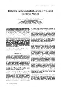
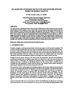
normal data is used in training. Fig. 1 presents the histogram of the covering similarity values (left column) for the ’normal’ (blue) and ’attack’ (red) data, the ordered similarity values in increasing order (middle column) for the ’normal’ (blue dotted line) and attack data (red, plain line) and the ROC curve (right column). In this figure, the top row corresponds to a situation for which 10% of the normal data has been randomly selected for training, the middle raw when the initial 10% of training data has been enriched using 12% of the remaining normal data corresponding to the lowest covering similarity scores, and finally, the bottom row corresponds to an enrichment of the initial 10% training data using 28% of the remaining normal data. From top to bottom, we show that the model improves its capacity to separate attack data from normal data: the AUC value that is initially .81, reaches .94 when 22% of the ’normal’ data is used as training and 1.0 when 38% of the ’normal’ data is used as training. In the middle column, we see that the similarity scores for the normal data progressively tangent the 1 constant curve (maximal similarity value), while, for the attack data, it stays globally much lower, although is increases slightly when the size of the training set increases. Figure 2 presents for this experiment the AUC value obtained by the algorithm as the enrichment of the training data increases. 5 different runs have been carried out, each one being initialized by randomly drawing 10% of the normal data. The grey area corresponds to the +1/-1 standard deviation, and the blue dotted line is the average curve. We can see on this figure that the SC4ID algorithm improves quite rapidly until reaching a perfect separation of the normal and attack data when 38% of the normal data is used, what ever the initialization is. This is a major and very promising result, since the instance selection that is performed directly from the covering similarity scores is working particularly well on the UNM data. 4.2

The ADFA-LD dataset

The second experiment involves a much more recent benchmark dataset for HIDS, designed by the Australian Centre OF Cyber Security (ACCS). According to the authors, the ADFA-LD dataset [27], [33] has been designed to reflect modern hacking techniques, while using modern patched software as its backbone. It is composed with a train set composed with 833 normal sequences, a validation set composed with 4373 normal sequences and a set of 746 attack sequences partitioned in 6 categories referred to as HydraFTP, Hydra-SSH, Adduser, Java-Meterpreter, Meterpreter and Webshell. Similarly to the UNM experiment, the experimental protocol for this data set is as follows : 1) initialization: select the 833 sequences of the normal train data to build the ’normal’ model, i.e. the initial set of normal data, S , against which the covering similarity will be evaluated. 2) Evaluation: for all the remaining normal and all attack sequences, s, evaluate the covering similarity S (s, S). Then rank the normal data according to their similarity

JOURNAL OF LATEX CLASS FILES, VOL. 14, NO. 8, DECEMBER 2017

6

Fig. 1. UNM dataset: histogram of the covering similarity distributions Sc (s, S) (left column), ranked covering similarity Sc (s, S) (middle column), ROC curves (right column), when 10% (top row), 22% (middle row) and 38% (bottom row) of the normal data is used for training.

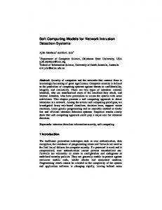
scores. Finally evaluate the ROC curve and assessment metrics. 3) From the previously ranked normal data, select 100 sequences of normal data with the worse similarity score, S100 , update the normal model S := S ∪ S100 and loop in step 2 until 50% of the normal data is used in training. When only the 833 normal train sequences are used to train SC4ID, one get the histogram of similarity scores given in top of Fig. 3. A red peak of maximal similarity (1.0) exists, meaning that some attack data (actually 32

sequences) are exact subsequences of the 833 normal train data. When we remove these 32 attack sequences, one notice a smaller remaining red peak with high covering similarity close to 1.0. This peak corresponds to 11 attack sequences that have a covering of size 2, i.e. that are composed with two subsequences that belongs to the set of training data. This situation for which attack sequences can be exact subsequences of normal data is a bit surprising and one may wonder how this can be possible. We do not have investigated the nature of such subsequences and do not argue further about a potential mix-up between attack and

JOURNAL OF LATEX CLASS FILES, VOL. 14, NO. 8, DECEMBER 2017

7

Fig. 2. UNM dataset: AUC curves as a function of the size of the training set in percent for 5 distinct runs. The average curve is shown in dotted line. The grey filled area shows the +1/-1 std curves.

normal sets. Rather, we take the opportunity to highlight an obvious limitation of SC4ID: it is completely blind to this kind of situation. Complementary approaches are required to address specifically this issue if any. Fig. 4 presents the histogram of the covering similarity values (left column) for the ’normal’ (blue) and ’attack’ (red) data, the ordered similarity values in increasing order (middle column) for the ’normal’ (blue dotted line) and attack data (red, plain line) and two ROC curves (right column): the black plain line curve corresponds to the situation where all the attack data is kept, the blue dotted line corresponds to the situation where the 32 attack sequences that are exact subsequences of the 833 normal train data are removed. In this figure, the top row corresponds to the situation where only the 833 normal train sequences are used for training, the middle raw when the initial 833 sequences have been enriched using 500 sequences of the remaining normal data and having the lowest covering similarity, and finally the bottom row corresponds to a an enrichment of the initial 833 train sequences using the 1000 sequences of the remaining normal data having the lowest covering similarity. From top to bottom, we show that the model improves its capacity to separate attack data from normal data: the AUC value that is initially .84/.88, reaches .93/.97 when 500 normal sequences have been added to the initial training data and .96/99 when 1000 normal sequences have been added to the 833 initial training set. Similarly to what we have observed for the UMN dataset, in the middle column, we see that the similarity score for the normal data progressively tangents the 1 constant curve, while, for the attack data, it stays globally much lower, although is increases slightly. Fig. 5 presents for this experiment the AUC values for the algorithm as the enrichment of the training data

Fig. 3. Histogram of the covering similarity for normal validation data (blue), and attack data (red). Top: all the attacks are considered, notice the red pick with maximal similarity, 1.0, corresponding to attacks that are exact subsequences of the train sequences. Bottom: the same histogram when the 32 attacks with covering similarity equal to 1.0 are removed. Notice the remaining small peak of high similarity close to 1.0

JOURNAL OF LATEX CLASS FILES, VOL. 14, NO. 8, DECEMBER 2017

8

Fig. 4. ADFA-LD dataset: histogram of the covering similarity distributions Sc (s, S) (left column), ranked covering similarity Sc (s, S) (middle column), ROC curves (right column), when 833 normal data (top row), 833 + 500 normal data (middle row) and 333 + 1000 normal data (bottom row) is used for training.

increases. We can see on this figure that the SC4ID algorithm improves rapidly until reaching an almost perfect separation (when the attacks that are subsequences of the train data have been removed) of the normal and attack data when 1400 normal data have been used to enrich the initial 833 training set. Here again, the instance selection that is performed directly from the covering similarity scores is working particularly well. Nevertheless, we notice after adding 1400 sequences that the algorithm is a little less efficient with a AUC value that drops from .975/.998 to

.971/.992. The explanation is that a remaining few attacks (precisely the 11 sequences mentioned earlier that have a covering of size 2 when using only the 833 train sequences) become subsequences of some of the lastly added normal subsequences to train set. The similarity for these few attacks reaches the maximal value, namely 1.0, and they cannot be separated anymore, hence a lower AUC value.

JOURNAL OF LATEX CLASS FILES, VOL. 14, NO. 8, DECEMBER 2017

Fig. 5. ADFA-LD dataset: AUC curves as a function of the number of normal data added to the initial training set. The black plain line correspond to the situation for which the sequences of attacks which are an exact subsequence of a normal data have been removed. The blue dotted line corresponds corresponds to the case where no sequence of attacks has been removed.

9

of the enrichment step. Ror the ADFA-LD dataset (which is much larger in size than UNM dataset), It varies around an average of about 900 seconds with a large standard deviation (about 100 sec.). From the analysis of the logs collected during our experiments, we found that i) the time required to construct the suffix tree is marginal, ii) the elapsed time progressively shifts from the extraction of the coverings for the validation normal sequences to the extraction of the coverings for the attack data. This is due partly to the fact that the number of normal validation data to evaluate decreases, but also because the extraction is becoming much easier for the normal data because the size of the covering becomes very small in average as the enrichment progresses (similarity scores tangent the maximal similarity score for normal data). Due to the variability in length of the sequences that are added to the train data, it is difficult to go deeper into this analysis. Nevertheless, these curves show that, i) for the various configurations corresponding to each step of the enrichment process, the extraction of the S -optimal coverings is bounded in time and ii) the two addressed problems are processed in a quite reasonable elapsed time.

5

Fig. 6. Elapsed time in second during each steps of the enrichment procedure for the UNM (dotted black line) and ADFA-LD (plain blue line) datasets.

4.3

Runtime consideration

Fig. 6 presents the elapsed time in second for each iteration of the enrichment process carried out for the UNM (dotted curve) and ADFA-LD (plain curve) datasets. Each step of this process involves the construction of a suffix tree based on the train (normal) data, S , and the extraction of the S -optimal coverings for the validation (normal) and attack data. These curves have been obtained on a Intel(R) Core(TM) i7-6700HQ CPU @ 2.60GHz laptop running an Ubuntu 16.10 release. Notice that between two successive tests, the train data increases by one sequence for the UNM dataset and 100 sequences for the ADFA-LD dataset; conversely the validation (normal) dataset is reduced by one sequence and 100 sequences respectively. Hence, as the enrichment increases, the number of S -optimal coverings to extract decreases. We observe that the elapsed time is quite stable, around 450 seconds, for the UNM dataset and rather independent

D ISCUSSION AND CONCLUSION

The UNM dataset, although relatively old and somehow outdated, gives a general view of the capability of the SC4ID algorithm to separate normal data from attacks sequences. The fact that the first results highlighted on the UNM dataset are still observable on a much recent and reputed difficult benchmark such as the ADFA-LD dataset is particularly promising. In both cases, the instance selection ability of SC4ID allows for rapidly improving the separability of attack sequences from the normal ones. When the train data is sufficiently representative of the normal activity expressed in terms of system call sequences, the algorithm achieves a quasi perfect separation. We have shown that, if this perfect separation is not obtained on the ADFA-LD dataset, this is because some attack sequences actually correspond exactly to some subsequences of the normal sequences that are used to train the model. If this kind of overlap is suppressed then one can expect a perfect separability as show in Fig. 5. To give some hints about how SC4ID compares with the state of the art methods that have been tested on the ADFALD dataset, we report hereinafter the results we found in the recent literature: In [35] bag of words and vector space model with tf and tf-idf weightings were used. Authors report a bit less than 80% in accuracy for a false positive rate of 30%. In [36] a one-cass SVM has been evaluated using a feature vector composed with n-grams of length 5. The authors report an average accuracy of 70% at a False Positive Rate of about 20%. In [37] a 10 fold cross-validation supervised classification (which is a much easier task than the anomaly detection task we are considering in this work, since attack data is used to train the classifiers) has been conducted. Authors report a AUC=0.93 for the best tested method (k-nn with k=3), using an ’enhanced’ vector space model with n-grams (n=2,3,4,5). In [24], an ensemble deep learning approach (LSTM) has been evaluated. Authors report an AUC value of 0.928 for an

JOURNAL OF LATEX CLASS FILES, VOL. 14, NO. 8, DECEMBER 2017

aggregating method that is somehow questionable, and an AUC value of 0.859 for a classical voting ensemble method. This implies that for a single LSTM model, the AUC value would be at most .86. In [27] a combinatorics ’semantic’ approach has been set up. It requires enumerating all phrases of 5 words with gaps, each word consisting of any subsequence (of any length) extracted from the train data (we estimate at about 6.101 6 the number of such phrases). The authors, actually the designers of the ADFA-LD dataset, report an AU C = .95 after several weeks of computing effort. In [38], authors have proposed to reduce system call traces by applying trace abstraction techniques. The approach consists mainly to reduce the size of the alphabet, by using meta-symbols, i.e. subsets that partition the alphabet. Authors report a 12.69% false positive rate for a 100% true positive rate when using a HMM model. This shows that the SC4ID algorithm is quite competitive, as far as enough normal training data is used. Its main advantages compared to the previously mentioned approaches are: i) it is parameter free, except for the decision threshold σ . Hence no assumption need to be made on the data, no windowing, no maximal length for the n-grams that are taken into account, no hidden architecture (HMM, LSTM) need to be defined, no meta parameters (SVM, RF) need to be tuned, etc. ii) It is incremental: the elements of the covering are progressively discovered and never modified afterwards. Hence the algorithm can be easily setup for an on-line exploitation. iii) The covering similarity is a very efficient measure that can (and should) be used to decide if a given normal sequence should be part of the training data or not. Basically, when a lot of normal data is available, which is actually the case in the HIDS application scope, it offers a data selection scheme with a stop condition that can be easily set up according to the middle columns of Fig. 1 and 4. When the ranked normal similarity curve tangent the 1-constant horizontal line, SC4ID will not improve furthermore its capability to isolate abnormal data, abnormality being clearly defined in the context of the considered set of normal data. iv) its applicability, in particular, it runs easily on common hardware for medium size problems. However, we have pointed out a limitation of the SC4ID algorithm: it cannot separate sequences that are exact subsequences of the training set. Of course, one may challenge, in the context of anomaly detection, whether it makes sense to consider that a subsequence of a normal sequence is possibly abnormal. Any algorithm that exploits historical data to provide a regressive or predictive scoring would also fail to correctly handle such situation. As a perspective, we can expect a speed up of the algorithm when trace abstraction techniques, such as described in [38], are used to reduce system call traces. This speedup, hopefully, could potentially be obtained without losing (too much) on the accuracy. Parallelization of the algorithm is also an issue that can be addressed, in particular in the context of a suffix array implementation.

10

Finally, one may ask whether the covering similarity is able to offer some useful solutions in other domain such as bioinformatics, sequence mining (clustering, classification), etc. In particular, the pair-wise similarity defined in Eq. 2 could be tested in various context, to evaluate the robustness and generality aspect of the concept of sequence covering.

R EFERENCES [1] [2] [3] [4] [5] [6] [7]

[8] [9]

[10]

[11]

[12]

[13]

[14]

[15]

[16]

[17] [18] [19]

A. Regev and T. Darsan, “Tinba malware reloaded and attacking banks around the world,” SecurityIntelligence, 2014. D. Bonderud, “Tinba number five takes aim at asia-pacific finance,” SecurityIntelligence, 2016. ——, “Malware top 10: Conficker grabs top spot, tinba takes second,” SecurityIntelligence, 2016. V. Chandola, A. Banerjee, and V. Kumar, “Anomaly detection: A survey,” ACM Comput. Surv., vol. 41, no. 3, pp. 15:1–15:58, Jul. 2009. [Online]. Available: http://doi.acm.org/10.1145/1541880.1541882 K. A. Scarfone and P. M. Mell, “Sp 800-94. guide to intrusion detection and prevention systems (idps),” Gaithersburg, MD, United States, Tech. Rep., 2007. S. Forrest, S. A. Hofmeyr, A. Somayaji, and T. A. Longstaff, “A sense of self for unix processes,” in Proceedings 1996 IEEE Symposium on Security and Privacy, May 1996, pp. 120–128. H.-J. Liao, C.-H. Richard Lin, Y.-C. Lin, and K.-Y. Tung, “Review: Intrusion detection system: A comprehensive review,” J. Netw. Comput. Appl., vol. 36, no. 1, pp. 16–24, Jan. 2013. [Online]. Available: http://dx.doi.org/10.1016/j.jnca.2012.09.004 M. H. Bhuyan, D. K. Bhattacharyya, and J. K. Kalita, “Network anomaly detection: Methods, systems and tools,” IEEE Communications Surveys Tutorials, vol. 16, no. 1, pp. 303–336, First 2014. E. Hodo, X. J. A. Bellekens, A. Hamilton, C. Tachtatzis, and R. C. Atkinson, “Shallow and deep networks intrusion detection system: A taxonomy and survey,” CoRR, vol. abs/1701.02145, 2017. [Online]. Available: http://arxiv.org/abs/1701.02145 S. A. Hofmeyr, S. Forrest, and A. Somayaji, “Intrusion detection using sequences of system calls,” J. Comput. Secur., vol. 6, no. 3, pp. 151–180, Aug. 1998. [Online]. Available: http://dl.acm.org/citation.cfm?id=1298081.1298084 Y. Wang, J. Wong, and A. Miner, “Anomaly intrusion detection using one class svm,” in Proceedings from the Fifth Annual IEEE SMC Information Assurance Workshop, 2004., June 2004, pp. 358– 364. Y. Yao, Y. Wei, F. x. Gao, and G. Yu, “Anomaly intrusion detection approach using hybrid mlp/cnn neural network,” in Sixth International Conference on Intelligent Systems Design and Applications, vol. 2, Oct 2006, pp. 1095–1102. S. Budalakoti, A. N. Srivastava, and M. E. Otey, “Anomaly detection and diagnosis algorithms for discrete symbol sequences with applications to airline safety,” IEEE Transactions on Systems, Man, and Cybernetics, Part C (Applications and Reviews), vol. 39, no. 1, pp. 101–113, Jan 2009. S. Coull, J. Branch, B. Szymanski, and E. Breimer, “Intrusion detection: A bioinformatics approach,” in Proceedings of the 19th Annual Computer Security Applications Conference, ser. ACSAC ’03. Washington, DC, USA: IEEE Computer Society, 2003, pp. 24–. [Online]. Available: http://dl.acm.org/citation.cfm?id= 956415.956442 A. Kundu, S. Sural, and A. K. Majumdar, “Database intrusion detection using sequence alignment,” International Journal of Information Security, vol. 9, no. 3, pp. 179–191, Jun 2010. [Online]. Available: https://doi.org/10.1007/s10207-010-0102-5 M. D. Wan, S. H. S. Huang, and J. Yang, “Finding the longest similar subsequence of thumbprints for intrusion detection,” in 20th International Conference on Advanced Information Networking and Applications - Volume 1 (AINA’06), vol. 1, April 2006, pp. 6 pp.–. A. Sureka, “Kernel based sequential data anomaly detection in business process event logs,” CoRR, vol. abs/1507.01168, 2015. [Online]. Available: http://arxiv.org/abs/1507.01168 Y. Qiao, X. W. Xin, Y. Bin, and S. Ge, “Anomaly intrusion detection method based on hmm,” Electronics Letters, vol. 38, no. 13, pp. 663–664, Jun 2002. J. Hu, Host-Based Anomaly Intrusion Detection. Berlin, Heidelberg: Springer Berlin Heidelberg, 2010, pp. 235–255. [Online]. Available: https://doi.org/10.1007/978-3-642-04117-4 13

JOURNAL OF LATEX CLASS FILES, VOL. 14, NO. 8, DECEMBER 2017

[20] R. Jain and N. S. Abouzakhar, “Hidden markov model based anomaly intrusion detection,” in 2012 International Conference for Internet Technology and Secured Transactions, Dec 2012, pp. 528–533. [21] K. K. Gupta, B. Nath, and K. Ramamohanarao, “Conditional random fields for intrusion detection,” in Advanced Information Networking and Applications Workshops, 2007, AINAW ’07. 21st International Conference on, vol. 1, May 2007, pp. 203–208. [22] L. Taub, “Applying conditional random fields to payload anomaly detection with crfpad,” in 2013 Proceedings of IEEE Southeastcon, April 2013, pp. 1–5. [23] M. Sheikhan, Z. Jadidi, and A. Farrokhi, “Intrusion detection using reduced-size rnn based on feature grouping,” Neural Computing and Applications, vol. 21, no. 6, pp. 1185–1190, Sep 2012. [Online]. Available: https://doi.org/10.1007/s00521-010-0487-0 [24] J. Kim, J. Kim, H. L. T. Thu, and H. Kim, “Long short term memory recurrent neural network classifier for intrusion detection,” in 2016 International Conference on Platform Technology and Service (PlatCon), Feb 2016, pp. 1–5. [25] K. Rieck and P. Laskov, “Language models for detection of unknown attacks in network traffic,” Journal in Computer Virology, vol. 2, no. 4, pp. 243–256, Feb 2007. [Online]. Available: https://doi.org/10.1007/s11416-006-0030-0 [26] B. Orisaniya and D. Patel, “Evaluation of modified vector space representation using adfa-ld and adfa-wd datasets.” Journal of Information Security, vol. 6, pp. 250–264, 2015. [27] G. Creech and J. Hu, “A semantic approach to host-based intrusion detection systems using contiguousand discontiguous system call patterns,” IEEE Transactions on Computers, vol. 63, no. 4, pp. 807– 819, April 2014. [28] P. Bieganski, J. Riedl, J. V. Cartis, and E. F. Retzel, “Generalized suffix trees for biological sequence data: applications and implementation,” in 1994 Proceedings of the Twenty-Seventh Hawaii International Conference on System Sciences, vol. 5, Jan 1994, pp. 35– 44. [29] E. Ukkonen, “On-line construction of suffix trees,” Algorithmica, vol. 14, no. 3, pp. 249–260, Sep 1995. [Online]. Available: https://doi.org/10.1007/BF01206331 [30] U. Manber and G. Myers, “Suffix arrays: A new method for on-line string searches,” in Proceedings of the First Annual ACM-SIAM Symposium on Discrete Algorithms, ser. SODA ’90. Philadelphia, PA, USA: Society for Industrial and Applied Mathematics, 1990, pp. 319–327. [Online]. Available: http://dl.acm.org/citation.cfm?id=320176.320218 [31] M. I. Abouelhoda, S. Kurtz, and E. Ohlebusch, “Replacing suffix trees with enhanced suffix arrays,” Journal of Discrete Algorithms, vol. 2, no. 1, pp. 53 – 86, 2004, the 9th International Symposium on String Processing and Information Retrieval. [Online]. Available: http://www.sciencedirect.com/ science/article/pii/S1570866703000650 [32] S. Forrest, “Intrusion detection dataset. university of new mexico (unm),” 1998. [Online]. Available: http://www.cs.unm. edu/∼immsec/systemcalls.htm [33] G. Creech and J. Hu, “Generation of a new ids test dataset: Time to retire the kdd collection,” in 2013 IEEE Wireless Communications and Networking Conference (WCNC), April 2013, pp. 4487–4492. [34] E. N. Yolacan, “Learning from sequential data for anomaly detection,” Ph.D. dissertation, Boston (Mass.) : Northeastern University, 2014. [35] M. Xie and J. Hu, “Evaluating host-based anomaly detection systems: A preliminary analysis of adfa-ld,” in 2013 6th International Congress on Image and Signal Processing (CISP), vol. 03, Dec 2013, pp. 1711–1716. [36] M. Xie, J. Hu, and J. Slay, “Evaluating host-based anomaly detection systems: Application of the one-class svm algorithm to adfa-ld,” in 2014 11th International Conference on Fuzzy Systems and Knowledge Discovery (FSKD), Aug 2014, pp. 978–982. [37] B. Borisaniya and D. Patel, “Evaluation of modified vector space representation using adfa-ld and adfa-wd datasets,” Journal of Information Security, vol. 6, pp. 250–264, 2015. [38] S. S. Murtaza, W. Khreich, A. Hamou-Lhadj, and S. Gagnon, “A trace abstraction approach for host-based anomaly detection,” in 2015 IEEE Symposium on Computational Intelligence for Security and Defense Applications (CISDA), May 2015, pp. 1–8.

11