The determination of the sensor orientation by sequential estimation based ... pair with reference data indicates the achieved accuracy of the algorithmic approach. .... of landmarks (natural features) at positions with high level gradients in two.
International Archives of Photogrammetry and Remote Sensing 1994, Vol. 30, Part 5, pp. 206-213.
SEQUENTIAL ESTIMATION OF SENSOR ORIENTATION FOR STEREO IMAGES SEQUENCES Thomas P. Kersten and Emmanuel P. Baltsavias Swiss Federal Institute of Technology, Institute of Geodesy and Photogrammetry ETH-Hoenggerberg, CH-8093 Zurich, Switzerland ISPRS Commission V, IC Working Group V/III
KEY WORDS: Image Sequence Analysis, On-line Triangulation, Robot Vision, Sequential Estimation ABSTRACT Among a wide variety of sensing technologies vision systems are capable to derive a mobile robot’s relationship and orientation with respect to the surrounding environment. In this paper, we present an algorithmic approach to derive sensor orientation from image sequences acquired by a binocular vision-based mobile “robot”, which moves in an office, sensing its environment. The data acquisition, the extraction of characteristic features in the image frames, and the tracking and matching of the landmarks along the sequence is described. The determination of the sensor orientation by sequential estimation based on Givens transformations is demonstrated using the tracked data of the test sequence. The results of the vision system’s calibration and of the sensor orientation are presented. Finally, a comparison of the sensor orientation of the last stereo pair with reference data indicates the achieved accuracy of the algorithmic approach. 1. INTRODUCTION For time-constrained robot vision applications careful tuning and optimised interaction of the system’s hardware, algorithmic complexity, software engineering, and task performance for accuracy processing of image sequences including image analysis and object space feature positioning is required. In this respect, errors in image acquisition and processing cannot be totally avoided. Thus, robust 3-D positioning techniques, error detection, and analysis are necessary components to derive sensor orientation from image sequences for vision-based robot navigation applications. Requirements, i.e. practical speed, performance, and noise tolerance, for a photogrammetric robot vision system are discussed in El-Hakim (1985). The total time required to process image sequences and to perform vision operations (such as target extraction and tracking) and sensor orientation, depends specially on the requirements of each application. For real time vision-based robot navigation all operations for one image frame must be processed in less than the frame acquisition time (1/25 of a second). Therefore, to perform such robot vision applications, some operations will be performed by hardware, and others by software. Special-purpose hardware modules can be up to 1000 times faster than regular software. Although we are aware that very fast (e.g. video rate) solutions to positioning problems with affordable computer hardware still require substantial simplification of the measurement problem at hand, we nevertheless present in this paper a general solution for sequential point positioning and sensor orientation, based on the bundle solution. The investigations, described in the paper, are performed to test our algorithms for robot vision applications and not to present a real time system for vision-based robot navigation. The presented algorithmic approach includes self-calibration parameters for systematic error modelling and statistical tests for blunder detection. The sequential estimation procedure applies Givens transformations for updating of the upper triangle of the reduced normal equations. Blais (1983) introduced Givens transformations for photogrammetric applications and Gruen and Kersten (1992) for robot vision applications. We use Givens transformations as opposed to a Kalman update because in robotics the covariance update of the parameter vector is not required at every stage and then, if at all, only at relatively sparse increments. Moreover, the varying size of the parameter vector (addition and deletion of new object points, addition of frame exterior orientation parameters) leads to poor computational performance of the Kalman filter. A number of sequential estimation algorithms have been compared to each other in the past. Firstly, the TFU algorithm (Triangular Factor Update), which updates directly the upper triangle of the reduced normal equations, was found to perform much better than the Kalman form of updating both in terms of computing times and storage requirement (Gruen, 1982, Wyatt, 1982). Later, the Givens transformations were found to be superior, in general, to the TFU (Runge, 1987, Holm, 1989) in computational performance, data space requirement, and in the ease of mechanization and software implementation. In the most image sequence analysis applications the Kal-man filter is used. In Matthies et al. (1989) the Kalman filter is used to estimate a depth map from image sequences. Typical for this approach is that depth estimates and uncertainty values are computed at each pixel of minified (256 x 256 pels) video frames and that these estimates are refined 1
International Archives of Photogrammetry and Remote Sensing 1994, Vol. 30, Part 5, pp. 206-213.
incrementally over time. The good performance of the Kalman filter is due to the fact that only one parameter (depth value) constitutes the state vector and is updated. Errors in orientation and calibration of the video frames and thus correlations between different elements of the depth map are not considered. Also, only lateral motion of the CCDcamera is assumed. Zhang and Faugeras (1990) use the Kalman update mechanism to track object motion in a sequence of stereo frames. They track object features, called “tokens” (line segments for example), in 3-D space from frame to frame and estimate the motion parameters of these tokens in a unified way (they also integrate a model of motion kinematics). Their state vector consists thus of three angular velocity, three translational velocity and three translational acceleration parameters of each object and in addition six line segment parameters for each 3-D line representation. As before, the tokens are treated independently here, which allows the state vector for estimation to remain small in size and may result in straightforward parallelization for any number of tokens. Hahn (1991) estimates 3-D egomotion from a monosequence of 160 images, acquired with a CCD camera mounted on a driven car, updating the solution vector (3 coordinates and 3 rotational components) by the 3-D Kalman filter.
Figure 1: Hardware setup of the mobile “robot” A stereo-vision system integrated in addition to a GPS receiver and an inertial system into a mobile mapping workstation is used in Edmundson and Novak (1992) to navigate a van through the GPS loss-of-lock period. The orientation of the cameras along the sequence are determined sequentially with Givens transformations without square roots. 2. HARDWARE SETUP FOR THE DATA ACQUISITION Our mobile “robot” (Figure 1) consists of a vision system, a data storage system, a camera synchronisation unit, a pattern generator, and a mobile platform with four wheels. Two synchronised standard SONY-XC77CE CCD cameras with a FUJINON 9 mm lens are rigidly mounted on the mobile platform. The base of the two cameras was 56 cm. The motion of the robot’s platform was performed by an operator and could be visually controlled by the display of one camera’s video signal on a standard monitor, which was placed on the top of the platform. As the data rate of the vision system is about 13 MB/sec and real-time storage devices like memory or video disks for fast storage of long digital image sequences is still expensive, the image data is intermediately being stored on two analog U-matic video recorders and digitized later. To be capable to read corresponding image frames from the two video tapes, a pattern generator adds a binary pattern to all image frames coding a sequential number (Figure 4).
2
International Archives of Photogrammetry and Remote Sensing 1994, Vol. 30, Part 5, pp. 206-213.
3. DETERMINATION OF THE SENSOR ORIENTATION The determination of the sensor orientation for the sequence is achieved by the cyclic procedure as illustrated in Figure 2: (1) image acquisition and digitization, (2) image processing to extract characteristic features (landmarks), (3) tracking and matching of the landmarks, and (4) sequential estimation for the sensor orientation including blunder detection and removal. Before the data processing for the sensor orientation, a calibration of the vision system was performed.
Figure 2: Procedure for the determination of sensor orientation 3.1. Image acquisition and digitization The robot was moved by an operator through the office environment imaging the office objects. In the beginning and at the end of the sequence, a 3-D testfield was imaged to perform an accuracy test later. The robot’s path in the office environment is illustrated in Figure 3. The image sequences were digitized from the video tapes on a PCbased digitizer station, which was equipped with a Matrox MVP frame grabber board and a card giving access to the remote control port of the video recorder for digitizing the sequences automatically using the play and rewind mode. The intermediate storage of the image sequences on videotape instead of direct digitization causes loss of quality and reduction of the positional accuracy by 30% (Maas, 1992). In total, 742 image frames of each sequence were digitized. This yields a time of 29.7 seconds and the usage of 195 MB disk space per sequence. Because of the motion effects in the image frames, which caused problems in the extraction of characteristic features from the full frames, we used fields for the further processing of the sequences. To reduce the amount of data actually only the odd fields were used.
Figure 3: Dimensions of the office room and robot’s path (planview) 3
International Archives of Photogrammetry and Remote Sensing 1994, Vol. 30, Part 5, pp. 206-213.
V
C
T AP
P
Ch
σ
r
Accuracy from check points1)
Precision from adjustment
[µm] Object space [mm]
1 2 3 4 5
1 1 2 2 2 V C T AP P Ch
1)
1 2 1 2 1
9 9 9 9 0
874 859 878 864 878
63 63 62 62 62
1292 1262 1306 1278 1312
0.70 1.02 0.73 0.97 6.57
Version Camera Type (1=Full, 2=Half frame) Number of additional parameters Number of points Number of check points
σX 0.14 0.21 0.15 0.19 1.31 r σ σXYZ σxy µ XYZ µ xy
σY 0.14 0.21 0.15 0.19 1.31
Image space [µm]
σZ 0.35 0.52 0.37 0.49 3.35
σx 0.7 0.9 0.7 0.9 5.7
σy 0.4 0.9 0.5 0.7 5.7
Object space [mm]
µX 0.23 0.30 0.26 0.29 3.15
µY 0.22 0.30 0.20 0.21 3.47
Image space [µm]
µZ 0.32 0.58 0.41 0.54 5.93
µx 0.6 0.8 0.7 0.8 11.1
µy 0.6 0.8 0.5 0.7 10.9
Redundancy Standard deviation of measured image coord. a posteriori Theoretical precision in object space Theoretical precision in image space Empirical accuracy in object space Empirical accuracy in image space
Values obtained after a spatial similarity transformation of all check point coordinates onto their reference values.
Table 1: Results of the calibration for the robot vision system 3.2. Calibration of the vision system In addition to the test sequence, images were acquired for calibrating the two SONY cameras. In the calibration, 9 additional parameters, which model interior orientation (location of the principal point and the camera constant) and other systematic errors (a scale factor in x, a shear, two parameters for radial and two parameters for decentering distortion) were determined. Furthermore, the results of the calibration permit an estimation of the accuracy that can be achieved in the sensor’s orientation with the vision system. The 3-D testfield was imaged from four different camera positions and the image data was stored on video tape. Two images at each camera position were acquired with rolls of 0 and 90 degrees. In the digitized images, the pixel coordinates of up to 123 testfield targets were measured in all images by least squares template matching, while reference coordinates for the targets were obtained by theodolite measurements. The observations were processed in a bundle adjustment with self-calibration. The results of the bundle adjustment and the comparison with check points, as an independent verification of the accuracy, are shown in Table 1. All versions are computed with 8 control points. Version 1 and 2 summarize the results of the calibration for camera 1, while version 3 and 4 present the results for camera 2. For both cameras, a calibration with the full (type 1) and half image frames (type 2) was performed. The comparison of the results of the different image size shows that the calibration of the half frames yielded an accuracy deterioration in the
Figure 4: Image frame of the sequence with characteristic landmarks (binary pattern in the left upper image corner) 4
International Archives of Photogrammetry and Remote Sensing 1994, Vol. 30, Part 5, pp. 206-213.
order of a factor 1.3, which was attributed to the smaller target size. The empirical accuracy measures (µX, µY, µZ), which are computed after a spatial similarity transformation onto their check point coordinates, shows that an accuracy of better than half a millimeter was obtained for all calibrations. This corresponds to a relative accuracy of about 1:12,000 in the object space, while in image space an accuracy in the order of 1/15th of the pixel spacing for the half and 1/20th of the pixel spacing for full image frames could be achieved. The comparison of the results of all versions (1-4) with additional parameters and no additional parameters (Version 5) shows that the accuracy improvement, which was obtained by self-calibration with the set of 9 additional parameters, is in the order of 10. This demonstrates significantly the necessity of camera calibration for accurate robot vision applications. 3.3. Landmark extraction After image acquisition, extraction of landmarks (natural features) at positions with high level gradients in two orthogonal directions is performed by using the Foerstner interest operator (Foerstner and Guelch, 1987). The parameters of the operator were set such that points with large grey level gradients in two orthogonal directions and centers of small circles were selected. In particular, the following parameters were used: 5 x 5 window size, gradients computed by a 3 x 3 Sobel, point localisation using a 9 x 9 neighbourhood, and non-maxima suppression using a 21 x 21 window. Approximately 50 - 60 points were selected in the left image field of the first pair. The corresponding points in the right image were detected by geometrically constrained least squares matching (Baltsavias, 1991) using a 9 x 9 pixels patch size, two shifts and two scales as geometric parameters, and gain and offset radiometric corrections. Then, the points were tracked independently in each image sequence, as explained in section 3.4. This tracking stopped after approximately 50 images (called a subsequence thereafter), i.e. 2 seconds acquisition time, because since the cameras were moving, new objects appeared in the images, and the selected landmarks had to be updated. Thus, the Foerstner operator was applied to the new area in the last image of the left sequence, and the corresponding points in the right image were found again with image matching. The last image pair was then used as the first pair of a new subsequence of 50 images, i.e. the new points and the old points that were still in the last image pair were tracked independently. This procedure continued until corresponding points in all images of both sequences were detected. 3.4. Tracking of landmarks and blunder detection For processing of the first stereo pair, one of the following approaches can be used: (i) if points with known 3-D object coordinates exist, the sensor orientation and the 3-D coordinates of all landmarks in the first image pair can be determined by bundle adjustment, or (ii) if no such coordinates exist, the sensor orientation must be known (possibly in an arbitrary local coordinate system) and the 3-D coordinates of the landmarks can be determined through spatial intersection. In our test the first approach has been used. In this case, the known points were the testfield points. For processing of the following stereo pairs, the landmarks are tracked in each image along the sequence using an adaptive least-squares matching approach, which also delivers accuracy estimates and permits blunder detection. The previously mentioned matching algorithm was used again, but this time without constraints as the sensor orientations were unknown. This matching method can track features, only when their displacement from image to image within the sequence is small, in general less than 4 - 5 pixels. This last number also depends on the patch size that is used for matching (in this case 9 x 9 pixels), and it increases with increasing patch size but less than linearly. Since the geometric and radiometric differences between sequentially acquired images were small, matching was performed with no radiometric corrections, and only two shifts as geometric parameters. These simplifications did not lead to a deterioration of the matching accuracy and increased the processing speed significantly (120 matched points per second on a Sun SparcStation 10). A small patch size is generally required in tracking applications, in order to reduce disturbances by changing background (in case of moving objects) and occlusions (due to the movement of the sensors), and to speed-up the computations. The average displacement from image to image was approximately 2 pixels, with variations among the different subsequences (range of average displacement was 0.6 - 2.5 pixels). However, maximum displacements of ca. 7 pixels were observed, and with correct convergence indeed. Problems occur with selected points that are centers of small circles when there are large scale changes within the image sequence. This was the case at a part of the sequence where the robot was moving frontally towards the objects. The initially small circles were becoming larger and larger and since the patch size was constant and small, the patch gradually fell within the inner of the circle where there was no texture. Some of these matchings may have failed, but most probably the majority of the matchings were side-minima, and thus wrong. From this point of view, for tracking it is better to use features that are less scale sensitive, like corners. The problem with the circles can be avoided, if the patch size can vary within the sequence, but this solution is cumbersome as it requires a signal analysis, in order to determine the size of the circle. Another solution would be to select with the Foerstner operator the points (i) every so many images within the sequence (here every 50 images was used) such that the scale differences between first and last image within each subsequence are small, and (ii) in the whole image and not only in the new areas. Thus, centers of large circles would not be selected because of the small window size of the Foerstner operator. In total, about 38,000 out of possible 44,000 matchings, i.e. 88%, were performed for each camera. The losses are due to points that disappear from the images due to the sensor motion, occlusions, possible poor approximate values, and multiple solutions due to lack of texture. In each subsequence, 58 points on the average were tracked, with the range
5
International Archives of Photogrammetry and Remote Sensing 1994, Vol. 30, Part 5, pp. 206-213.
being 35 - 73. Out of these points, only 44 points on the average, i.e. 75%, could be tracked until the last image of each subsequence with the range being 23 - 67. Even in the case of 23 points, the number of points was sufficient for estimation of the sensor orientation. The matching results were further tested with the aim of automatic detection and rejection of blunders. This is essential because wrong tracking may influence the estimation of the sensor orientation, even if blunder detection is used in the on-line triangulation. The criteria that can be used for quality analysis are: standard deviation of unit weight from the least square matching, correlation coefficient between the template and the patch, number of iterations, x-shift (i.e. change from the approximate values), standard deviation of x-shift, y-shift, standard deviation of y-shift, and the sizes of the shaping parameters (two scales, two shears). The shaping parameters were not used in this case, nor the number of iterations. After matching, the median (M) and the standard deviation of the mean absolute difference from the median s(MAD) were computed for each criterion from all points of each image pair that were tracked. The median and the s(MAD) were used instead of the average and the standard deviation because they are robust against blunders. For each criterion, the threshold for the rejection of a point was defined as M+N s(MAD). N is generally selected to be 3 for all criteria with the exception of the two shifts which should be left to vary more (N = 5) because they depend on the distance of the landmarks from the sensors. In this case, a value of N = 3 would result in very strict thresholds, so for all criteria N = 5 was used. A point was rejected (i) when one of its criterion did not fulfil the aforementioned threshold (relative threshold derived from the image statistics), or (ii) one of its criteria did not fulfil a loosely set threshold. The matching program provides global statistics for all matchings of each subsequence, and these statistics were used to set the global thresholds. The same N and absolute thresholds were used for all image pairs of both sequences. The percentage of points that were rejected for each tracking from image to image was in the range 0 - 20%, with a mean value of ca. 5%. The aforementioned problem with patches within large circles, i.e. patches with low texture, could be solved by using this blunder detection test. These points were rejected because of large values of the standard deviations of the two shifts. 3.5. Sequential estimation and data snooping The sensor orientation was computed in the On-Line Triangulation System OLTRIS (Kersten et al., 1992). In OLTRIS, it is possible to perform sequential update with Givens transformations and simultaneous adjustment with Cholesky factorization and back-substitution. During the introduction of the image data observations the pixel coordinates of each tracked point were transformed to image coordinates with the pixel-to-image coordinate transformation (Beyer, 1992). Before the introduction of the observations into the normal equation system, a rough blunder detection was implemented by rejecting all observations (less than 0.1%) with a 5 times higher standard deviation, as estimated by the matching algorithm, than the sigma a priori (3 µm). Also, the effects of systematic errors, which were determined in the calibration, were compensated for by the use of the additional parameters to the introduced image coordinates.
Figure 5: Computed path of the mobile “robot” in its environment 6
International Archives of Photogrammetry and Remote Sensing 1994, Vol. 30, Part 5, pp. 206-213.
Due to the huge number of image coordinates observations, in total 66,656 points, and its resulting long computation time, the sequence of 742 stereo pairs was divided in ten subsequences (sections with a number of stereo image pairs between 65 and 105). To obtain a reliable connection between these subsequences an overlap of 5 pairs was chosen. The sequence started with known camera stations of the first stereo pair, which were computed from object points of the testfield. The characteristic points in the first stereo pair, which were detected by the Foerstner operator, were computed by intersection, while the following sensor orientations were computed by spatial resection. All these computed values were introduced as weighted observations into the normal equation system sequentially. The solution of the first two stereo pairs was computed in a simultaneous adjustment, in order to obtain stable start conditions of the sequence. At that early stage of the sequence, the cpu-time for the adjustment was very small. For the following sequence pair, the solution vector is updated by sequential estimation when all new observations of the current stereo pair are added. The solution vector consists of the sensor orientation of each acquired image frame and of the 3-D object point coordinates. After each sequential update of the normals, all observations were tested for blunders. For blunder detection, which is particularly important in automated measurement systems, Baarda’s data snooping has become standard in photogrammetric applications and is implemented in OLTRIS. The computation of the related test criteria , (i = 1, . . . , n), requires the computation of both, the residual vector v and the diagonal elements of the Qvv-matrix. In Gruen (1985) it has been shown how the full Qvv-matrix can be efficiently computed or updated with the Givens approach. Baarda’s data snooping assumes that gross errors in the observation data set have low corrrelations. Accordingly, the five observations with the biggest blunders above the test criterion 3.3 were excluded without checking the correlations in the Qvv-matrix after each data snooping and a new update was performed afterwards. To avoid the influence of observations with gross errors in the following stereo pairs, the residuals of the excluded observations were tested whether they were larger than five times sigma a priori. If that was the case, it was assumed that the points were wrongly tracked and that the observations of these points in the following images would also be wrong. Consequently, these observations were not introduced in the normals when adding a new stereo pair. But the visual checking of some excluded blunders showed that some detected blunders were correctly matched and their residuals were small, which led to the conclusion that high correlations among the blunders must occur. In future investigations the parts of Qvvmatrix, which are related to the detected blunders, has to be computed to check the correlations of the blunders. Figure 5 shows the computed path of the mobile “robot” in its environment. This figure illustrates that due to the error propagation and incrementation the sensor orientations starts varying slightly as the number of introduced stereo image pairs increases. This could be expected, because no control points were used in the sequence. However, the determination of the sensor orientation could be performed more precisely and reliably if well distributed control points in the robot’s environment could be used.
Figure 6: CPU-times for introducing one additional image point (top) and for testing one image point in the data snooping procedure (bottom) 7
International Archives of Photogrammetry and Remote Sensing 1994, Vol. 30, Part 5, pp. 206-213.
The data processing in OLTRIS was performed on a Sun SPARCStation 10. For the computation of each subsequence an elapsed time of 4 up to 23 hours was needed on this workstation. This indicates clearly, that the used hardware power is far away from performing in real time vision based robot navigation using this algorithm. But as aforementioned in this practical test we wanted to demonstrate the capability of our algorithmic approach to derive sensor orientation from image sequences. Computing times (CPU) for the sequential updating of the solution vector when including the observations of one additional image point and for the testing of one image point observation in the data snooping procedure are illustrated in Figure 6. The plotted line shows the increase of CPU-time consumption for the first 25 stereo pairs of the sequence depending on the number of observations. The driven distance of the mobile platform was 1.425 m with a mean velocity of 48 mm/s. The achieved accuracy was tested with the following comparison. The sensor orientation of the last image frame pair, determined from the last step of the sequential estimation, was compared with a bundle solution of the last stereo pair using the points of the 3-D testfield as control points. The difference of the two solutions, which permits an overall estimation of the performance of the presented approach, are summarized in Table 2. Camera
dx [mm]
dy [mm]
dz [mm]
left
16.6
20.7
6.7
right
2.8
36.3
-1.4
average
9.7
28.5
2.7
Table 2: Difference of the sensor orientation of the last stereo pair to reference values In both solutions the effect of systematic errors were compensated. As it can be seen from Table 2 the biggest difference to the reference values is in the height coordinate. This is also indicated in Figure 5 by the variation in y (height). There is no clear explanation for this and theoretically it should not be so. The variation in y starts at about image pair no. 280 and lasts up to image pair no. 610, probably due to the reduced number of points and their possible bad distribution in these image pairs. 4. CONCLUSIONS AND FURTHER WORK In a practical test with a binocular vision-based mobile platform the capability of our algorithmic approach to derive sensor orientation from image sequences without control points is demonstrated. Although the computation time was far away from real time, the results of determining the sensor orientations were promising. Without the sequential estimation including the blunder detection, i.e. if nonstrict solutions like spatial resection were used, the error propagation and incrementation after 742 pairs would be larger than the one indicated in Table 2 . However, in future this approach has to be tested practically with image sequences acquired in different environments under modified conditions. The capability of sensor fusion for navigation tasks should also be considered. From the algorithmic point of view the feature extraction and the blunder detection has to be improved and optimized concerning robustness and cpu-time consumption. Especially for blunder detection, different methods and strategies should be tested due to the aforementioned constraints of Baarda’s data snooping. Due to its excessive cpu-time consumption the strict data snooping must be replaced by approximate procedures to increase the speed of our algorithmic approach. For an aerial triangulation bundle system Gruen (1979) showed how to avoid the enormous computational effort if approximate values obtained from reliability models for the are applied. To make the approach more robust, the correlations between blunders should be checked, a denser point configuration in the image frames should be guaranteed, and the error detection should be improved by rejecting wrongly tracked points in all subsequent frames after the frame where tracking failure was detected, and points that appear in only one sequence. Furthermore, it must be investigated whether video rate or only a lower frame rate, i.e. each fifth frame, is needed for robust and reliable sequential estimation of sensor orientation. Thus, the less stereo frames are necessary the more cputime could be saved. 5. ACKNOWLEDGMENTS K. R. Holm supported the development of OLTRIS significantly. H.-G. Maas provided the software for the digitizer station and assisted together with M. Virant in the digitization of the sequence. D. Stallmann provided the software for the Foerstner interest operator. Their support is gratefully acknowledged.
8
International Archives of Photogrammetry and Remote Sensing 1994, Vol. 30, Part 5, pp. 206-213.
6. REFERENCES Baltsavias, E.P., 1991: Multiphoto Geometrically Constrained Matching. Ph. D. dissertation, ETH Zurich, Institute of Geodesy and Photogrammetry, Mitteilungen Nr. 49, December, 221 p. Beyer, H.A., 1992: Geometric and Radiometric Analysis of a CCD-Camera Based Photogrammetric Close-Range System. Ph. D. dissertation, ETH Zurich, Institute of Geodesy and Photogrammetry, Mitteilungen Nr. 51, May, 186 p. Foerstner, W., Guelch, E., 1987: A Fast Operator for Detection and Precise Location of Distinct Points, Corners and Centers of Circular Features. Proceedings of ISPRS Intercommission Conference on “Fast Processing of Photogrammetric Data”, Interlaken, Switzerland, June 2-4, pp. 281-305. Blais, J.A.R., 1983: Linear Least-Squares Computations Using Givens Transformations. The Canadian Surveyor. Vol. 37, No. 4, pp. 225-233. Deriche, R., Faugeras, O., 1990: Tracking Line Segments. Proceedings of the First European Conference of Computer Vision, Antibes, France, April, pp. 259-268. Edmundson, K.L., Novak, K., 1992: On-Line Triangulation for Autonomous Vehicle Navigation. Paper presented at XVII ISPRS Congress, Washington, D.C., USA, 2-14 August 1992. International Archives of Photogrammetry and Remote Sensing, Vol. XXIX, Part B5, Commission V, pp. 916-922. El-Hakim, S.F., 1985: A Photogrammetric Vision System for Robots. Photogrammetric Engineering & Remote Sensing, Vol. 51, No. 5, pp. 545-552. Gruen, A., 1979: Gross Error Detection in Bundle Adjustment. Paper presented at the Aerial Triangulation Symposium, Brisbane, Australia, October 15-17. Gruen, A., 1985: Algorithmic Aspects in On-Line Triangulation. Photogrammetric Engineering and Remote Sensing, Vol. 51. No. 4, pp. 419-436. Gruen, A., Kersten, Th., 1992: Sequential Estimation in Robot Vision. Paper presented at XVII ISPRS Congress, Washington, D.C., USA, 2-14 August 1992. International Archives of Photogrammetry and Remote Sensing, Vol. XXIX, Part B5, Commission V, pp. 923-931. Hahn, M., 1991: 3-D Egomotion from Long Image Sequences. Proceedings of the Second Int. Workshop on High Precision Navigation, Stuttgart/Freudenstadt, Nov. 1991, pp. 241-251. Holm, K.R., 1989: Test of Algorithms for Sequential Adjustment in On-Line Phototriangulation. Photogrammetria, 43, pp. 143-156. Kersten, Th., Gruen, A., Holm, K.R., 1992: On-Line Point Positioning with Single Frame Camera Data. DoD Final Technical Report, No. 7, Swiss Federal Institute of Technology, IGP-Bericht, No. 197, ETH-Zurich, Switzerland. Maas, H.-G., 1992: Digitale Photogrammetrie in der dreidimensionalen Strömungsmesstechnik. Ph. D. dissertation, ETH Zurich, Institute of Geodesy and Photogrammetry, Mitteilungen Nr. 50, February, 140 p. Matthies, L.M., Szeliski, R., Kanade, T., 1989: Kalman Filter-based Algorithms for Estimating Depth from Image Sequences. Int. Journal of Computer Vision, Vol. 3, No. 3. pp. 209-238. Runge, A., 1987: The Use of Givens Transformation in On-Line Triangulation. Proceedings of ISPRS Intercommission Conference on “Fast Processing of Photogrammetric Data”, Interlaken, Switzerland, June 2-4, pp. 179-192. Wyatt. A.H., 1982: On-Line Triangulation - An Algorithmic Approach. Master Thesis, Department of Geodetic Sciences and Surveying, The Ohio State University, Columbus, Ohio. Zhang, Z., Faugeras, O., 1990: Motion Tracking in a Sequence of Stereo Frames. Proceedings 9th European Conference of Artificial Intelligence, Stockholm, Sweden, August, pp. 747- 752.
9