variate conditionally heteroskedastic dynamic regression models, our results ...... although in that case we must use a robust (sandwich) formula to obtain J 751 ...
Sequential estimation of shape parameters in multivariate dynamic models Dante Amengual CEMFI, Casado del Alisal 5, E-28014 Madrid, Spain Gabriele Fiorentini Università di Firenze and RCEA, Viale Morgagni 59, I-50134 Firenze, Italy Enrique Sentana CEMFI, Casado del Alisal 5, E-28014 Madrid, Spain February 2012
Abstract Sequential maximum likelihood and GMM estimators of distributional parameters obtained from the standardised innovations of multivariate conditionally heteroskedastic dynamic regression models evaluated at Gaussian PML estimators preserve the consistency of mean and variance parameters while allowing for realistic distributions. We assess the e¢ ciency of those estimators, and obtain moment conditions leading to sequential estimators as e¢ cient as their joint maximum likelihood counterparts. We also obtain standard errors for the quantiles required in VaR and CoVaR calculations, and analyse the e¤ects on these measures of distributional misspeci…cation. Finally, we illustrate the small sample performance of these procedures through Monte Carlo simulations. Keywords: Elliptical Distributions, E¢ cient Estimation, Systemic Risk, Value at Risk. JEL: C13, C32, G11
We would like to thank Manuel Arellano, Christian Bontemps, Olivier Faugeras, Javier Mencía, Francisco Peñaranda, Marcos Sanso and David Veredas, as well as audiences at CEMFI, CREST, Princeton, Rimini, Toulouse, the Finance Forum (Granada, 2011) the Symposium of the Spanish Economic Association and the Conference in honour of M. Hashem Pesaran (Cambridge, 2011) for useful comments and suggestions. Of course, the usual caveat applies. Amengual and Sentana gratefully acknowledge.…nancial support from the Spanish Ministry of Science and Innovation through grants ECO 2008-00280 and 2011-26342.
1
Introduction Nowadays it is well documented and widely recognised that the distribution of returns on
…nancial assets such as stocks, bonds or currencies is usually rather leptokurtic, even after controlling for volatility clustering e¤ects. Nevertheless, many empirical researchers continue to use the Gaussian pseudo-maximum likelihood (PML) estimators advocated by Bollerslev and Wooldridge (1992) among others because they remain root-T consistent for the conditional mean and variance parameters so long as those moments are correctly speci…ed and the fourth moments are bounded. However, academics and …nancial market participants are often interested in features of the distribution of asset returns beyond its conditional mean and variance. In particular, the Basel Capital Adequacy Accord forced banks and other …nancial institutions to develop models to quantify all their risks accurately. In practice, most institutions chose the so-called Value at Risk (VaR) framework in order to determine the capital necessary to cover their exposure to market risk. As is well known, the VaR of a portfolio of …nancial assets is de…ned as the positive threshold value V such that the probability of the portfolio su¤ering a reduction in wealth larger than V over some …xed time interval equals some pre-speci…ed level
< 1=2. Similarly,
the recent …nancial crisis has highlighted the need for systemic risk measures that assess how an institution is a¤ected when another institution, or indeed the entire …nancial system, is in distress. Given that the probability of the joint occurrence of several extreme events is regularly underestimated by the multivariate normal distribution, any such measure should de…nitely take into account the non-linear dependence induced by the non-normality of …nancial returns. A rather natural modelling strategy is to specify a parametric leptokurtic distribution for the standardised innovations of the vector of asset returns, such as the multivariate Student t, and to estimate the conditional mean and variance parameters jointly with the parameters characterising the shape of the assumed distribution by maximum likelihood (ML) (see for example Pesaran, Schleicher and Za¤aroni (2009) and Pesaran and Pesaran (2010)). Elliptical distributions such as the multivariate t are attractive in this context because they relate mean-variance analysis to expected utility maximisation (see e.g. Chamberlain (1983), Owen and Rabinovitch (1983) and Berk (1997)). Moreover, they generalise the multivariate normal distribution, but at the same time they retain its analytical tractability irrespective of the number of assets. However, the problem with non-Gaussian ML estimators is that they often achieve e¢ ciency gains under cor1
rect speci…cation at the risk of returning inconsistent parameter estimators under distributional misspeci…cation, as shown by Newey and Steigerwald (1997). Unfortunately, semiparametric estimators of the joint density of the innovations su¤er from the curse of dimensionality, which severely limits their use when the number of assets under consideration is moderately large. Another possibility would be semiparametric methods that impose the assumption of ellipticity, which retain univariate nonparametric rates regardless of the cross-sectional dimension of the data, but asymmetries in the true distribution will again contaminate the resulting estimators of conditional mean and variance parameters. Sequential estimators of shape parameters that use the Gaussian PML estimators of the mean and variance parameters as …rst step estimators o¤er an attractive compromise because they preserve the consistency of the …st two conditional moments under distributional misspeci…cation, while allowing for more realistic conditional distributions. The focus of our paper is precisely the econometric analysis of sequential estimators obtained from the standardised innovations evaluated at the Gaussian PML estimators. Speci…cally, we consider not only sequential ML estimators, but also sequential generalised method of moments (GMM) estimators based on certain functions of the standardised innovations. Although we could easily extend our results to any multivariate distribution, to keep the exposition simple we focus on elliptical distributions. We illustrate our general results with several examples that nest the normal, including the Student t and the original Kotz (1975) distribution, as well as some rather ‡exible families such as scale mixtures of normals and polynomial expansions of the multivariate normal density, both of which could form the basis for a proper nonparametric procedure. We explain how to compute asymptotic standard errors of sequential estimators that take into account the sampling variability of the Gaussian PML estimators on which they are based. We also exploit the expressions of the standard errors to assess the relative e¢ ciency of sequential estimators, and obtain the optimal moment conditions that lead to sequential MM estimators which are as e¢ cient as their joint ML counterparts. Although we explicitly consider multivariate conditionally heteroskedastic dynamic regression models, our results obviously apply in univariate contexts as well as in static ones. We then analyse the use of our sequential estimators in the computation of commonly used risk management measures such as VaR, and recently proposed systemic risk measures such as Conditional Value at Risk (CoVaR) (see Adrian and Brunnermeier (2011)). In particular,
2
we compare our sequential estimators to nonparametric estimators, both when the parametric conditional distribution is correctly speci…ed and also when it is misspeci…ed. Our analytical and simulation results indicate that the use of sequential ML estimators of ‡exible parametric families of distributions in estimating those risk measures o¤ers substantial e¢ ciency gains, while incurring in small biases. The rest of the paper is organised as follows. In section 2, we introduce the model, present closed-form expressions for the score vector and the conditional information matrix, and derive the asymptotic variances of the ML and Gaussian PML estimators. Then, in section 3 we introduce the sequential ML and GMM estimators, and compare their e¢ ciency. In section 4, we study the in‡uence of those estimators on risk measures under both correct speci…cation and misspeci…cation, and derive asymptotically valid standard errors. A Monte Carlo evaluation of the di¤erent parameter estimators and risk measures can be found in section 5. Finally, we present our conclusions in section 6. Proofs and auxiliary results are gathered in appendices.
2
Theoretical background
2.1
The dynamic econometric model
Discrete time models for …nancial time series are usually characterised by an explicit dynamic regression model with time-varying variances and covariances. Typically the N dependent variables, yt , are assumed to be generated as: 1=2
yt = t ( 0 ) + t ( 0 )"t ; t ( ) = (zt ; It 1 ; ); (zt ; It 1 ; ); t( ) = where p
() and vech [ ()] are N
1 and N (N + 1)=2
1 vector of true parameter values
0,
denotes the information set available at t
zt are k contemporaneous conditioning variables, It 1, which contains past values of yt and zt , 1=2 t (
some particular “square root”matrix such that di¤erence sequence satisfying E("t jzt ; It
1 vector functions known up to the
1;
0)
E(yt jzt ; It 1 ; V (yt jzt ; It 1 ;
)
1=20 ( t
)=
= 0 and V ("t jzt ; It 0)
= 0) =
t( 0) t( 0)
1=2 t (
1
) is
t(
), and "t is a martingale
1;
0)
= IN . Hence,
:
(1)
To complete the model, we need to specify the conditional distribution of "t . We shall initially assume that, conditional on zt and It
1,
"t is independent and identically distributed as some
particular member of the spherical family with a well de…ned density, or "t jzt ; It s(0; IN ;
0)
for short, where
are some q additional shape parameters. 3
1;
0;
0
i:i:d:
2.2
Elliptical distributions
A spherically symmetric random vector of dimension N , "t , is fully characterised in Theorem 2.5 (iii) of Fang, Kotz and Ng (1990) as "t = et ut , where ut is uniformly distributed on the unit sphere surface in RN , and et is a non-negative random variable independent of ut , whose distribution determines the distribution of "t . The variables et and ut are referred to as the generating variate and the uniform base of the spherical distribution. Often, we shall also refer to & t = "t 0 "t , which trivially coincides with e2t . Assuming that E(e2t ) < 1, we can standardise "t by setting E(e2t ) = N , so that E("t ) = 0 and V ("t ) = IN . If we further assume that E(e4t ) < 1, then Mardia’s (1970) coe¢ cient of multivariate excess kurtosis = E(& 2t )=[N (N + 2)]
1;
(2)
will also be bounded. Some examples of elliptical distributions that we use to illustrate our general results are: p Gaussian: "t = & t ut is distributed as a standardised multivariate normal if and only if & t is a chi-square random variable with N degrees of freedom. Since this involves no additional parameters, we shall identify the normal distribution with 0 = 0. p p 2 Student t: "t = t = t ut is distributed as a standardised multivariate Student t if and only if
t
is a chi-square random variable with N degrees of freedom, and
variate with mean
and variance 2 , with ut ,
and
t
is a Gamma
t
mutually independent. Therefore, & t
will be proportional to an F random variable with N and
degrees of freedom. In this case, we
t
de…ne
as 1= , which will always remain in the …nite range [0; 1=2) under our assumptions. p Kotz : "t = & t ut is distributed as a standardised Kotz if and only if & t is a gamma random variable with mean N and variance N [(N + 2) + 2], so that the coe¢ cient of multivariate excess kurtosis itself is the shape parameter. Discrete scale mixture of normals: &t =
"t =
p
st + (1 + (1
& t ut is distributed as a DSMN if and only if st ){ ){
t
where st is an independent Bernoulli variate with P (st = 1) = , { is the variance ratio of the two components, which for identi…cation purposes we restrict to be in the range (0; 1] and
t
is
an independent chi-square random variable with N degrees of freedom. E¤ectively, in this case & t will be a two-component scale mixture of
20 s, N
4
with shape parameters
and {.
Polynomial expansion:
p
"t =
& t ut is distributed as a J th -order PE of the multivariate
normal if and only if & t has a density de…ned by h(& t ) = ho (& t ) PJ (& t ); where ho (& t ) = denotes the density function of a
1 N=2 & 2N=2 (N=2) t
1
exp
1 &t 2
2
with N degrees of freedom, and 2 3 J X PJ (& t ) = 41 + cj pgN=2 1;j (& t )5 j=2
is a J th order polynomial written in terms of the generalised Laguerre polynomial of order j and parameter N=2
1, pgN=2
1;j (:).
For example, the second and third order standardised Laguerre
polynomials are: pgN=2 pgN=2
1;2 (&)
1;3 (&)
s
=
s
=
2 N (N + 2) N (N + 2) 4
1 & + & 2 , and 4
12 N (N + 2) (N + 4) N +4 2 (N + 2) (N + 4) &+ & 8 8
N (N + 2) (N + 4) 24 As a result, the J
N +2 2
1 3 & . 24
1 shape parameters will be given by c2 ; c3 ; : : : ; cJ . The problem with
polynomial expansions is that h(& t ) will not be a proper density unless we restrict the coe¢ cients so that PJ (&) cannot become negative. For that reason, in Appendix C.1 we explain how to obtain restrictions on the cj ’s that guarantee the positivity of PJ (&) for all &. Figure 1 describes the region in (c2 ; c3 ) space in which densities of a 3rd -order PE are well de…ned for all &
0.
As we mentioned in the introduction, the multivariate Gaussian and Student t, which approaches the former as
! 0 (or
! 1) but has otherwise fatter tails, have been by far the
two most popular choices made by empirical researchers to model the conditional distribution of asset returns. But the other examples are more ‡exible even though they continue to nest the Gaussian distribution. In particular, the Kotz distribution reduces to the normal for
= 0, but
it can be either platykurtic ( < 0) or leptokurtic ( > 0). However, the density of a leptokurtic Kotz distribution has a pole at 0, which is a potential drawback from an empirical point of view. As for the DSMN, it approaches the multivariate normal when { ! 1,
! 1 or
! 0, although
near those limits the distributions can be radically di¤erent (see Amengual and Sentana (2011) 5
for further details). Nevertheless, the distribution of any scale mixture of normals is necessarily leptokurtic.1 Finally, the PE reduces to the spherical normal when cj = 0 for all j 2 f2; :::; Jg. Interestingly, while the distribution of "t is leptokurtic for a 2nd order expansion, it is possible to generate platykurtic random variables with a 3rd order expansion. Figure 2 plots the densities of a normal, a Student t, a platykurtic Kotz distribution, a DSMN and a 3rd -order PE in the bivariate case. Although they all have concentric circular contours because we have standardised and orthogonalised the two components, their densities can di¤er substantially in shape, and in particular, in the relative importance of the centre and the tails. They also di¤er in the degree of cross-sectional “tail dependence” between the components, the normal being the only example in which lack of correlation is equivalent to stochastic independence. In this regard, Figure 3 plots the so-called exceedance correlation between uncorrelated marginal components (see Longin and Solnik, 2001). As can be seen, the distributions we consider have the ‡exibility to generate very di¤erent exceedance correlations, which will be particularly important for systemic risk measures. It is also convenient to study the higher order moments of elliptical distributions. In this sense, it is easy to combine the representation of elliptical distributions above with the higher order moments of a multivariate normal vector in Balestra and Holly (1990) to prove that the third and fourth moments of a spherically symmetric distribution with V ("t ) = IN are given by E("t "t 0 E("t "t 0
"t ) = 0; "t "t 0 ) = E[vec("t "t 0 )vec0 ("t "t )] = ( +1)[(IN 2 +KN N )+vec (IN ) vec0 (IN )];
where Kmn is the commutation matrix of orders m and n and
is de…ned in (2). An alterna-
tive characterisation can be based on the higher order moment parameter of spherical random variables introduced by Berkane and Bentler (1986),
m(
), which Maruyama and Seo (2003)
relate to higher order moments as E[& m t j ] = [1 +
m(
m m )]E[& m t j0] where E[& t j0] = 2
m Y
(N=2 + j
1):
(3)
j=1
For the elliptical examples mentioned above, we derive expressions for
m(
) in Appendix C.2.
A noteworthy property of these examples is that their moments are always bounded, with the 1
Dealing with discrete scale mixtures of normals with multiple components would be tedious but fairly straightforward. As is well known, multiple component mixtures can arbitrarily approximate the more empirically realistic continuous mixtures of normals such as symmetric versions of the hyperbolic, normal inverse Gaussian, normal gamma mixtures, Laplace, etc. The same is also true of polynomial expansions.
6
exception of the Student t. Appendix C.3 contains the moment generating functions for the Kotz, the DSMN and the 3rd -order PE.
2.3
The log-likelihood function, its score and information matrix
Let
= ( 0 ; )0 denote the p + q parameters of interest, which we assume variation free.
Ignoring initial conditions, the log-likelihood function of a sample of size T for those values of P for which t ( ) has full rank will take the form LT ( ) = Tt=1 lt ( ), with lt ( ) = dt ( ) + c( ) + g [& t ( ); ], where dt ( ) =
1=2 ln j
t(
)j corresponds to the Jacobian, c( ) to the constant of
integration of the assumed density, and g [& t ( ); ] to its kernel, where & t ( ) = "t 0 ( )"t ( ), "t ( ) =
1=2 t
( )"t ( ) and "t ( ) = yt
t(
).
Let st ( ) denote the score function @lt ( )=@ , and partition it into two blocks, s t ( ) and s t ( ), whose dimensions conform to those of to show that if s t( ) =
t(
),
t(
and , respectively. Then, it is straightforward
), c( ) and g [& t ( ); ] are di¤erentiable
@dt ( ) @g [& t ( ); ] @& t ( ) + = [Zlt ( ); Zst ( )] @ @& @
elt ( ) est ( )
= Zdt ( )edt ( );
s t ( ) = @c( )=@ + @g [& t ( ); ] =@ = ert ( );
(4)
where @dt ( )=@
=
Zst ( )vec(IN )
@& t ( )=@
=
2fZlt ( )"t ( ) + Zst ( )vec "t ( )"t 0 ( ) g;
Zlt ( ) = @
0 t(
1 @vec0 [ 2
Zst ( ) = elt ( ; ) =
t(
)=@
0
and @vec [
t(
)] =@
t t(
( );
)] =@ [
1=20 t
1=20
( )
t
( )];
[& t ( ); ] "t ( );
est ( ; ) = vec @
1=20
)=@
0
[& t ( ); ] "t ( )"t 0 ( )
(5) IN ;
(6)
depend on the particular speci…cation adopted, and [& t ( ); ] =
2@g[& t ( ); ]=@&
(7)
can be understood as a damping factor that re‡ects the kurtosis of the speci…c distribution assumed for estimation purposes (see Appendix D.1 for further details). But since [& t ( ); ] is equal to 1 under Gaussianity, it is straightforward to check that s t ( ; 0) reduces to the multivariate normal expression in Bollerslev and Wooldridge (1992), in which case: edt ( ; 0) =
elt ( ; 0) est ( ; 0)
"t ( ) vec ["t ( )"t 0 ( )
= 7
IN ]
:
Given correct speci…cation, the results in Crowder (1976) imply that et ( ) = [e0dt ( ); ert ( )]0 evaluated at
0
follows a vector martingale di¤erence, and therefore, the same is true of the score
vector st ( ). His results also imply that, under suitable regularity conditions, the asymptotic p 1( distribution of the feasible, joint ML estimator will be T ( ^ T 0 ) ! N 0; I 0 ) , where I(
0)
= E[It (
0 )j 0 ],
It ( ) = V [st ( )jzt ; It Zt ( ) =
] = Zt ( )M( )Z0t ( ) =
1;
Zdt ( ) 0 0 Iq
Zlt ( ) Zst ( ) 0 0 0 Iq
=
ht ( ) denotes the Hessian function @st ( )=@
0
= @ 2 lt ( )=@ @
E [ht ( )jzt ; It
1;
];
; 0
and M( ) = V [et ( )j ].
The following result, which reproduces Proposition 2 in Fiorentini and Sentana (2010), contains the required expressions to compute the information matrix of the ML estimators: Proposition 1 If "t jzt ; It
1;
is i:i:d: s(0; IN ; ) with density exp[c( ) + g(& t ; )], then 1 0 Mll ( ) 0 0 0 Mss ( ) Msr ( ) A ; M( ) = @ 0 M0sr ( ) Mrr ( ) Mll ( ) = V [elt ( )j ] = mll ( )IN ;
Mss ( ) = V [ est ( )j ] = mss ( ) (IN 2 + KN N ) + [mss ( ) Msr ( ) = E[ est ( )e0rt ( )
]=
E @est ( )=@
Mrr ( ) = V [ ert ( )j ] = & t( ) N
0
E[ @ert ( )=@
1]vec(IN )vec0 (IN ); = vec(IN )msr ( ); 0
];
2@ [& t ( ); ] & t ( ) + [& t ( ); ] @& N n & t oi 2@ [& t ( ); ] & 2t ( ) N h 1+V [& t ( ); ] =E mss ( ) = N +2 N @& N (N + 2) & t( ) & ( ) @ [& t ( ); ] t 1 e0rt ( ) msr ( ) = E [& t ( ); ] = E N N @ 0 mll ( ) = E
2
[& t ( ); ]
=E
; + 1; :
Fiorentini, Sentana and Calzolari (2003) provide the relevant expressions for the multivariate standardised Student t; while the expressions for the Kotz distribution and the DSMN are given in Amengual and Sentana (2010).2
2.4
Gaussian pseudo maximum likelihood estimators of
If the interest of the researcher lied exclusively in , which are the parameters characterising the conditional mean and variance functions, then one attractive possibility would be to estimate a restricted version of the model in which
is set to zero. Let ~T = arg max LT ( ; 0) denote
2
The expression for mss ( ) for the Kotz distribution in Amengual and Sentana (2010) contains a typo. The correct value is (N + 2)=[(N + 2) + 2].
8
such a PML estimator of . As we mentioned in the introduction, ~T remains root-T consistent for
0
under correct speci…cation of
"t jzt ; It
1;
0
t(
) and
t(
) even though the conditional distribution of
is not Gaussian, provided that it has bounded fourth moments. The proof is based
on the fact that in those circumstances, the pseudo log-likelihood score, s t ( ; 0), is a vector martingale di¤erence sequence when evaluated at
0,
a property that inherits from edt ( ; 0).
The asymptotic distribution of the PML estimator of
is stated in the following result, which
reproduces Proposition 3.2 in Fiorentini and Sentana (2010):3 Proposition 2 If "t jzt ; It 1 ; 0 is i:i:d: s(0; IN ; 0 ) with 0p< 1, and the regularity conditions A.1 in Bollerslev and Wooldridge (1992) are satis…ed, then T (~T 0 ) ! N [0; C( 0 )], where C( ) = A
A( ) =
At ( ) =
E [h
E[ h
t(
1
( )B( )A
t(
; 0)j zt ; It
0
1;
] = Zdt ( )K(0)Z0dt ( );
B( ) = V [s t ( ; 0)j ] = E [Bt ( )j ] ;
and K ( ) = V [ edt ( ; 0)j zt ; It
But if
( );
; 0)j ] = E [At ( )j ] ;
Bt ( ) = V [ s t ( ; 0)j zt ; It
which only depends on
1
1;
]=
] = Zdt ( )K( )Z0dt ( );
1;
IN 0
0 ( +1) (IN 2 +KN N )+ vec(IN )vec0 (IN )
;
through the population coe¢ cient of multivariate excess kurtosis.
is in…nite then B(
0)
will be unbounded, and the asymptotic distribution of some
or all the elements of ~T will be non-standard, unlike that of ^T (see Hall and Yao (2003)).
3
Sequential estimators of the shape parameters
3.1
Sequential ML estimator of
Unfortunately, the normality assumption does not guarantee consistent estimators of other features of the conditional distribution of asset returns, such as its quantiles. Nevertheless, we can use ~T to obtain a sequential ML estimator of
as ~ T = arg max LT (~T ; ).4
Interestingly, these sequential ML estimators of tation. If & t(
0 ),
0
can be given a rather intuitive interpre-
were known, then the squared Euclidean norm of the standardised innovations,
would be i:i:d: over time, with density function N=2
h(& t ; ) =
(N=2)
N=2 1
&t
exp[c( ) + g(& t ; )]
(8)
3 Throughout this paper, we use the high level regularity conditions in Bollerslev and Wooldridge (1992) because we want to leave unspeci…ed the conditional mean vector and covariance matrix in order to maintain full generality. Primitive conditions for speci…c multivariate models can be found for instance in Ling and McAleer (2003). 4 In some cases there will be inequality constraints on , but for simplicity of exposition we postpone the details to Appendix D.1.
9
in view of expression (2.21) in Fang, Kotz and Ng (1990). Therefore, we could obtain the infeasible ML estimator of
by maximising with respect to this parameter the log-likelihood P function of the observed & t ( 0 )0 s, Tt=1 ln h [& t ( 0 ); ]. Although in practice the standardised
residuals are usually unobservable, it is easy to prove from (8) that ~ T is the estimator so obtained when we treat & t (~T ) as if they were really observed. Durbin (1970) and Pagan (1986) are two classic references on the properties of sequential ML estimators. A straightforward application of their results to our problem allows us to obtain the asymptotic distribution of ~ T , which re‡ects the sample uncertainty in ~T : Proposition 3 If "t jzt ; It 1 ; 0 is i:i:d: s(0; IN ; 0 ) with 0p< 1, and the regularity conditions A.1 in Bollerslev and Wooldridge (1992) are satis…ed, then T (~ T 0 ) ! N [0; F( 0 )], where F(
0)
Importantly, since C(
=I 0)
1
(
0)
+I
1
(
0 )I
0
(
0 )C( 0 )I
will become unbounded as
0
(
0 )I
1
(
0 ):
(9)
! 1, the asymptotic distribution of
~ T will also be non-standard in that case, unlike that of the feasible ML estimator ^ T . Expression (9) suggests that F(
0)
depends on the speci…cation adopted for the conditional
mean and variance functions. However, it turns out that the asymptotic dependence between estimators of F(
0)
and estimators of
is generally driven by a scalar parameter, in which case
does not depend on the functional form of
t(
) or
t(
). To clarify this point, it is
convenient to introduce the following reparametrisation: Reparametrisation 1 A homeomorphic transformation r(:) = [r01 (:); r20 (:)]0 of the conditional mean and variance parameters into an alternative set of parameters # = (#01 ; #02 )0 , where #2 is a scalar, and r( ) is twice continuously di¤ erentiable with rank[@r0 ( ) =@ ] = p in a neighbourhood of 0 , such that t ( ) = t (#1 ) ( t ) = #2 t (#1 )
8t;
(10)
8#1 :
(11)
with E[ln j
t (#1 )jj 0 ]
=k
Expression (10) simply requires that one can construct pseudo-standardised residuals "t (#1 ) =
1=2 t
(#1 )[yt
t (#1 )]
which are i:i:d: s(0; #2 IN ; ), where #2 is a global scale parameter, a condition satis…ed by most static and dynamic models.5
But given that we can multiply this parameter by some scalar
5
The only exceptions would be restricted models in which the overall scale is e¤ectively …xed, or in which it is not possible to exclude #2 from the mean. In the …rst case, the information matrix will be block diagonal between and , so no correction is necessary, while in the second case the general expression in Proposition 3 applies.
10
positive smooth function of #1 , k(#1 ) say, and divide
t (#1 )
by the same function without
violating (10), condition (11) simply provides a particularly convenient normalisation.6 We can then show the following result: Proposition 4 If "t jzt ; It 1 ; 0 is i:i:d: s(0; IN ; 0 ) with 0 < 1, the regularity conditions A.1 in Bollerslev and Wooldridge (1992) are satis…ed, and reparametrisation (1) is admissible, then F(
1 0 ) = Mrr (
1 0 )+Mrr (
0 0 )msr (
1 0 )Mrr (
0 )msr (
N 2#20
0)
2
C#2 #2 (#0 ;
0)
(12)
where
f2( +1) + N g 4#22 4 N is the asymptotic variance of the feasible PML estimator of #2 , while the asymptotic variance of the feasible ML estimator of is C#2 #2 (#; ) =
I
(
1 0 ) = Mrr (
1 0 )+Mrr (
0 0 )msr (
0 )msr (
with I #2 #2 ( ) =
1 2mss ( ) + N [mss ( )
1
1 0 )Mrr (
0)
N 2#20
2
I #2 #2 (
0 );
(13)
4#22 : msr ( )Mrr1 ( )m0sr ( )] N
In general, #1 or #2 will have no intrinsic interest. Therefore, given that ~ T is numerically invariant to the parametrisation of conditional mean and variance, it is not really necessary to estimate the model in terms of those parameters for the above expressions to apply as long as it would be conceivable to do so. In this sense, it is important to stress that neither (12) nor (13) e¤ectively depend on #2 , which drops out from those formulas. It is easy to see from (9) that I equality between I estimator of of
1(
0)
and F(
1( 0)
0)
0)
(
0)
if and only if I
F( (
0)
0)
regardless of the distribution, with
= 0, in which case the sequential ML
will be -adaptive, or in other words, as e¢ cient as the infeasible ML estimator
that we could compute if the & t (
msr (
I
0 0) s
were directly observed. This condition simpli…es to
= 0 when reparametrisation (1) is admissible.
A more interesting question in practice is the relationship between I
(
0)
and F(
0 ).
Theorem 5 in Pagan (1986) implies that p
T (~ T
^ T ) ! N [0; Y(
6
0 )] ;
Bickel (1982) exploited this parametrisation in his study of adaptive estimation in the iid elliptical case, and so did Linton (1993) and Hodgson and Vorkink (2003) in univariate and multivariate Garch-M models, respectively. As Fiorentini and Sentana (2010) show, in multivariate dynamic models with elliptical innovations (10) provides a general su¢ cient condition for the partial adaptivity of the ML estimators of #1 under correct speci…cation, and for their consistency under distributional misspeci…cation.
11
where Y(
0) = I
1
(
0 0 )I (
n ) C( 0
0)
I (
0)
I
(
0 )I
1
(
0 0 )I (
0)
1
o
I
(
0 )I
1
(
0 ):
Therefore, the sequential ML estimator will be asymptotically as e¢ cient as the joint ML estimator if and only if Y(
0)
= 0. If reparametrisation (1) is admissible, the scalar nature of
#2 implies that the only case in which I
(
0)
= F(
0)
with I
(
0)
6= 0 will arise when the
Gaussian PMLE of #2 is as e¢ cient as the joint ML.7 Otherwise, there will be an e¢ ciency loss.
3.2
Sequential GMM estimators of
If we can compute the expectations of L pute a sequential GMM estimator of where
q functions of & t , (:) say, then we can also com-
by minimising the quadratic form n0T (~T ; ) nT (~T ; ),
is a positive de…nite weighting matrix, and nt ( ; ) = [& t ( )]
Ef [& t ( )]j g. When
L > q, Hansen (1982) showed that if the long-run covariance matrix of the sample moment conditions has full rank, then its inverse will be the “optimal” weighting matrix, in the sense that the di¤erence between the asymptotic covariance matrix of the resulting GMM estimator and an estimator based on any other norm of the same moment conditions is positive semide…nite. This optimal estimator is infeasible unless we know the optimal matrix, but under additional regularity conditions, we can de…ne an asymptotically equivalent but feasible two-step optimal GMM estimator by replacing it with an estimator evaluated at some initial consistent estimator of
. An alternative way to make the optimal GMM estimator feasible is by explicitly taking
into account in the criterion function the dependence of the long-run variance on the parameter values, as in the single-step Continuously Updated (CU) GMM estimator of Hansen, Heaton and Yaron (1996). As we shall see below, in our parametric models we can often compute these GMM estimators using analytical expressions for the optimal weighting matrices, which we would expect a priori to lead to better performance in …nite samples. Following Newey (1984), Newey (1985) and Tauchen (1985), we can obtain the asymptotic covariance matrix of the sample average of the in‡uence functions evaluated at the Gaussian PML estimator, ~T , using the expansion 1 XT nt (~T ; t=1 T 7
0)
=
1 XT nt ( t=1 T
= (I; Nn A
1
)
0;
0)
1 XT t=1 T
p Nn T (~T nt ( 0 ; 0 ) s ( 0 ; 0)
The Kotz distribution provides a noteworthy example in which both msr (
12
0)
0)
+ op (1)
+ op (1)
= 0 and C#2 #2 (
0)
= I #2 #2 (
0 ).
where 1 XT E t=1 T !1 T
@nt ( 0 ; @ 0
Nn = lim Hence, we immediately get that p T XT nt (~T ; 0 ) lim V t=1 T !1 T
0
!
=(I; Nn A
where Gn Dn Dn0 B
= lim V
1
)
:
0
Gn Dn Dn0 B
I Nn A
nt ( 0 ; 0 ) s t ( 0 ; 0)
!
p
T XT t=1 T
T !1
0)
0
1
=En ;
(14)
:
An asymptotically equivalent way of dealing with parameter uncertainty replaces the original in‡uence functions nt ( ; ) with the residuals from their IV regression onto s t ( ; 0) using s t ( ) as instruments.8 More formally: Proposition 5 If "t jzt ; It 1 ; 0 is i:i:d: s(0; IN ; 0 ) with 0 < 1, and the regularity conditions A.1 in Bollerslev and Wooldridge (1992) are satis…ed, then the optimal sequential GMM ~ estimators based on nt (~T ; ) and n? t ( T ; ), where n? t ( ; ) = nt ( ; )
Nn A
1
s t ( ; 0);
will be asymptotically equivalent. In those cases in which reparametrisation (1) is admissible, we can obtain a third and much simpler equivalent procedure by using the residuals from the alternative IV regression of nt ( ; ) onto & t ( )=N
1 using [& t ( ); ]& t ( )=N
1 as instrument. Speci…cally,
Proposition 6 If "t jzt ; It 1 ; 0 is i:i:d: s(0; IN ; 0 ) with 0 < 1, the regularity conditions A.1 in Bollerslev and Wooldridge (1992) are satis…ed, and reparametrisation (1) is admissible, then the asymptotic variance of the sample average of nt ( ; ) = nt ( ; )
N & t( ) |n ( ) 2 N
where |n (
2)
= Cov nt ( ;
1 );
[& t ( );
2]
& t( ) N
1 ;
;
1
;
is equal to (14), which reduces to Gn
N N N (N + 2) |n (0)|0n ( ) + |n ( )|0n (0) + + 2 2 4
|n ( )|n ( )0 :
Finally, it is worth mentioning that when the number of moment conditions L is strictly larger than the number of shape parameters q, one could use the overidentifying restrictions statistic to test if the distribution assumed for estimation purposes is the true one. 8
See Bontemps and Meddahi (2011) for alternative approaches in moment-based speci…cation tests.
13
3.2.1
Higher order moments and orthogonal polynomials
The most obvious moments to use in practice to estimate the shape parameters are powers of & t . Speci…cally, we can consider the in‡uence functions: `mt ( ; ) =
2
&m t ( ) j=1 (N=2 + j
Qm m
1)
[1 +
m(
)]:
But given that for m = 1, expression (15) reduces to `1t ( ) = & t ( )=N have to start with m
(15) 1 irrespective of , we
2.
An alternative is to consider in‡uence functions de…ned by the relevant mth order orthogonal P h 9 Again, we have to consider m 2 because the polynomials pmt [& t ( ); ] = m h=0 ah ( )& t ( ).
…rst two non-normalised polynomials are always p0t [& t ( )] = 1 and p1t [& t ( )] = `1t ( ), which do
not depend on . Given that fp1t [& t ( )]; p2t [& t ( ); ]; :::; pM t [& t ( ); ]g is a full-rank linear transformation of [`1t ( ); `2t ( ; ); :::; `M t ( ; )], the optimal joint GMM estimator of
and
based on the …rst
M polynomials would be asymptotically equivalent to the corresponding estimator based on the …rst M higher order moments. The following proposition extends this result to optimal sequential GMM estimators that keep
…xed at its Gaussian PML estimator, ~T :
Proposition 7 If "t jzt ; It 1 ; 0 is i:i:d: s(0; IN ; 0 ) with E[& 2M t j 0 ] < 1, the regularity conditions A.1 in Bollerslev and Wooldridge (1992) are satis…ed, and reparametrisation (1) is admissible, then the optimal sequential estimator of based on the orthogonal polynomials of order 2, 3, :::, M is asymptotically equivalent to the analogous estimator based on the corresponding higher order moments, with an asymptotic variance that takes into account the sample uncertainty in ~T given by N N (N + 2) Gp + + |p ( )|p ( )0 2 4 where Gp is a diagonal matrix of order M 1 with representative element 8 9 m X m < h+k = X Y V [ pmt [& t ( ); ]j ] = ah ( )ak ( )[1 + h+k ( )]2h+k (N=2 + j 1) : ; j=1
h=0 k=0
and |p ( ) is an M
1 vector with representative element
Cov pmt [& t ( ); ]; [& t ( ); ]
& t( ) N
=
m X
hah ( )[1 +
h(
0 )]
h 2h+1 Y (N=2 + j N
1):
j=1
h=1
Importantly, these sequential GMM estimators will be not only asymptotically equivalent but also numerically equivalent if we use single-step GMM methods such as CU-GMM. By using additional moments, we can in principle improve the e¢ ciency of the sequential MM estimators, but the precision with which we can estimate 9
m(
) rapidly decreases with m.
Appendix B contains the expressions for the coe¢ cients of the second and third order orthogonal polynomials of the di¤erent examples we consider.
14
3.2.2
E¢ cient sequential GMM estimators of
Our previous GMM optimality discussion applies to a given set of moments. But one could also ask which estimating functions would lead to the most e¢ cient sequential estimators of taking into account the sampling variability in ~T . The following result answers this question by exploiting the characterisation of e¢ cient sequential estimators in Newey and Powell (1998): Proposition 8 If "t jzt ; It 1 ; 0 is i:i:d: s(0; IN ; 0 ) with 0 < 1, and the regularity conditions A.1 in Bollerslev and Wooldridge (1992) are satis…ed, then the e¢ cient in‡uence function is given by the e¢ cient parametric score of : s
j t(
; ) = s t( ; )
I0 (
0 )I
1
(
which is the residual from the theoretical regression of s t (
0 )s t ( 0)
; );
on s t (
(16)
0 ).
Importantly, the proof of this statement also implies that the resulting sequential MM estimator of
will achieve the e¢ ciency of the feasible ML estimator, which is the largest possible.
The reason is twofold. First, the variance of the e¢ cient parametric score s
j t( 0)
in (16)
coincides with the inverse of the asymptotic variance of the feasible ML estimator of
, ^T .
Second, this matrix is also the expected value of the Jacobian matrix of (16) with respect to . In those cases in which reparametrisation (1) is admissible, expression (16) reduces to s
j t(
; ) = s t( ; )
m0sr ( ) (1 + 2=N )mss ( )
[& t ( ); ]
1
& t( ) N
1 ;
(17)
which is once again much simpler to compute.
3.3
E¢ ciency comparisons
3.3.1
An illustration in the case of the Student t
In view of its popularity, it is convenient to illustrate our previous analysis in the case of the multivariate Student t. Given that when reparametrisation (1) is admissible Proposition 7 implies the coincidence between the asymptotic distributions of sequential MM estimators of
T
and
T,
which are the
based on the fourth moment and the second order polynomial,
respectively, we …rst derive the distribution of those estimators in the general case: Proposition 9 If "t jzt ; It 1 ; 0 is i:i:d: t(0; IN ; 0 ),pwith A.1 in Bollerslev and Wooldridge (1992) hold, then T ( T
15
0
> 8, and the regularity conditions 2 0 ) ! N 0; E` ( 0 )=H ( 0 ) and
p
T(
0)
T
! N 0; Ep ( 0)
+ N`0 (
E` (
0)
Ep (
0)
D` (
0)
= cov[s t (
G` (
0)
=
Gp (
0)
=
N` (
0)
=
Np (
0)
=
H(
= G` (
= Gp (
0)
0 )=H
+
2(
0)
, where 2N`0 (
0 )C( 0 )N` ( 0 )
1
0 )A
(
0 )D` ( 0 );
Np0 ( 0 )C( 0 )Np ( 0 );
4( 0 2)(N + 0 2) Ws ( 0 ); N ( 0 4)( 0 6) ( 0 2)2 (N + 6)(N + 4) ( 0 2)( 0 4) V [`2t ( 0 ; 0 )j 0 ] = 1 ; ( 0 4)2 N (N + 2) ( 0 6)( 0 8) 8( 0 2)2 (N + 0 2) V fp2t [& t ( 0 ); 0 ]j 0 g = G` ( 0 ) ; N ( 0 6)2 ( 0 4) 4( 0 2) cov[s t ( 0 ; 0 ); `2t ( 0 ; 0 )j 0 ] = Ws ( 0 ); N ( 0 4) 8( 0 2) covfs t ( 0 ; 0 ); p2t [& t ( 0 ); 0 ]j 0 g = Ws ( 0 ); N ( 0 4)( 0 6) 0 ; 0); `2t ( 0 ; 0 )j 0 ]
0 ) = cov[s t (
=
0 ; 0 ); `2t ( 0 ; 0 )j 0 ]
= covfs t (
0 ; 0 ); p2t [& t ( 0 ); 0 ]j 0 g
=
2 (
2 0
4)2
0
and Ws ( =E
1 @vec0 [ 2
0)
= Zd (
t ( 0 )] =@
0 )[0 1
vec[
t
0
; vec0 (IN )]0 = E[Zdt (
(
0 )]
0
0 0 0 0 )j 0 ][0 ; vec (IN )] 0 )j 0 ]
= E[Wst (
=
E f @dt ( )=@ j
The following proposition compares the e¢ ciency of these estimators of
0g :
(18)
to the sequential
ML estimator: Proposition 10 If "t jzt ; It addition A then J (
0)
G(
0 ),
1
(
1;
0
is i:i:d: t(0; IN ;
0 )Ws ( 0 )
=
(N + ( 0
0)
with
2)
0
4)
B
1
0
(
> 8, then F(
0)
0 )Ws ( 0 );
J(
0 ).
If in (19)
with equality if and only if
& t( 0) N
1
2(N + N( 0
0
2) 0 Ws ( 4)
0 )B
1
(
0 )s t ( 0 ; 0)
= 0 8t:
(20)
The …rst part of the proposition shows that sequential ML is always more e¢ cient than sequential MM based on the second order polynomial. Nevertheless, Proposition 8 implies that there is a sequential MM procedure that is more e¢ cient than sequential ML. Condition (19) is trivially satis…ed in the limiting case in which the Student t distribution is in fact Gaussian, and in dynamic univariate models with no mean. Also, it is worth mentioning that (20), which in turn implies (19), is satis…ed by most dynamic univariate Garch-M models (see Fiorentini, Sentana and Calzolari (2004)). More generally, condition (20) will hold in any model that satis…es reparametrisation (1). Given that I
(
0)
= 0 under normality from Proposition 1, it is clear that ~T will be as
asymptotically e¢ cient as the feasible ML estimator ^T when 16
0
= 0, which in turn is as e¢ cient
as the infeasible ML estimator in that case. Moreover, the restriction
0 implies that these
estimators will share the same half normal asymptotic distribution under conditional normality, although they would not necessarily be numerically identical when they are not zero. Similarly, the asymptotic distributions of increases when
= 0, since
0
case. However, while proportional to s t (
T
T
and ~
T( T)
for 2 < 3.3.2
0
T
and
0 ; 0),
4,
T
T
and
will also tend to be half normal as the sample size
is root-T consistent for
, which is 0 in the Gaussian
will always be as e¢ cient as ^T under normality because p2t [& t ( ); ] is T
will be less e¢ cient unless condition (20) is satis…ed.
Finally, note that since both G` ( from above,
T
0)
and Gp (
0)
will diverge to in…nity as
will not be root-T consistent for 4 T
0
0
converges to 8
8. Moreover, since
is in…nite
will not even be consistent in the interior of this range.
Asymptotic standard errors and relative e¢ ciency
Figures 4 to 6 display the asymptotic standard deviation (top panels) and the relative e¢ ciency (bottom panels) of the joint MLE and e¢ cient sequential MM estimator, the sequential MLE, and …nally the sequential GMM estimators based on orthogonal polynomials, obtained using the results in Propositions 4 and 7 under the assumption that reparametrisation (1) is admissible, which, as we mentioned before, covers most static and dynamic models. Figure 4 refers to the Student t distribution. For slight departures from normality ( < :02 or > 50) all estimators behave similarly. As
increases, the GMM estimators become relatively
less e¢ cient, with the exactly identi…ed GMM estimator being the least e¢ cient, as expected from Proposition 10. Notice, however, that when
approaches 12 the GMM estimator based on
the second and third orthogonal polynomials converges to the GMM estimator based only on the second one since the variance of the third orthogonal polynomial increases without bound. In turn, the variance of the estimator based on the second order polynomial blows up as converges to 8 from above, as we mentioned at the end of the previous subsection. Until roughly that point, the sequential ML estimator performs remarkably well, with virtually no e¢ ciency loss with respect to the benchmark given by either the joint MLE or the e¢ cient sequential MM. For smaller degrees of freedom, though, di¤erences between the sequential and the joint ML estimators become apparent, especially for values of
between 5 and 4.
The DSMN distribution has two shape parameters. In Figures 5a and 5b we maintain the scale ratio parameter { equal to .5 and report the asymptotic e¢ ciency as a function of the mixing probability parameter
. In contrast, in Figures 5c and 5d we look at the asymptotic 17
e¢ ciency of the di¤erent estimators …xing the mixing probability at
= 0:05. Interestingly, we
…nd that, broadly speaking, the asymptotic standard errors of the sequential MLE and the joint MLE are indistinguishable, despite the fact that the information matrix is not diagonal and the Gaussian PML estimators of
are ine¢ cient, unlike in the case of the Kotz distribution. As
for the GMM estimators, which in this case are well de…ned for every combination of parameter values, we …nd that the use of the fourth order orthogonal polynomial enhances e¢ ciency except for some isolated values of . Finally, Figures 6a to 6d show the results for the PE distribution, with c2 = 0 in the …rst two …gures and c3 = 0 in the other two. Again sequential MLE is very e¢ cient with virtually no e¢ ciency loss with respect to the benchmark. The GMM estimators are less e¢ cient, but the use of the fourth order polynomial is very useful in estimating c2 when c3 = 0 and in estimating c3 when c2 = 0.
3.4
Misspeci…cation analysis So far we have maintained the assumption that the true conditional distribution of the
standardised innovations "t is correctly speci…ed. Although distributional misspeci…cation will not a¤ect the Gaussian PML estimator of , the sequential estimators of if the true distribution of "t given zt and It
1
will be inconsistent
does not coincide with the assumed one. To focus
our discussion on the e¤ects of distributional misspeci…cation, in the remaining of this section we shall assume that (1) is true. Let us consider situations in which the true distribution is i:i:d: elliptical but di¤erent from the parametric one assumed for estimation purposes, which will often be chosen for convenience or familiarity. For simplicity, we de…ne the pseudo-true values of
as consistent roots of the ex-
pected pseudo log-likelihood score, which under appropriate regularity conditions will maximise the expected value of the pseudo log-likelihood function. We can then prove that: Proposition 11 If "t jzt ; It 1 ; '0 , is i:i:d: s(0; IN ), where ' includes # and the true shape parameters, but the spherical distribution assumed for estimation purposes does not necessarily nest the true density, and reparametrisation (1) is admissible, then the asymptotic distribution of the sequential ML estimator of , ~ T , will be given by p 1 1 T (~ T 1 ) ! N 0; Hrr ( 1 ; '0 )Er ( 1 ; '0 )Hrr ( 1 ; '0 ) ; where
1
solves E[ ert (#0 ; Hrr (
1 ; '0 )
1 )j '0 ]
= 0,
= MH rr (#0 ;
1 ; '0 );
MH rr ( ; ') = 18
E[ @ert ( )=@
0
'];
and Er (
+ 1] + N 0 g 4 1 O [Orr ( 1 ; '0 )] msr ( 1 ; '0 )0 mO sr ( 1 ; '0 )[Orr (
1 ; '0 )
= [Orr (
1 ; '0 )]
1
+
N f2[
0
1 ; '0 )]
1
;
with mO sr ( ; ') = E [ f [& t (#); ] [& t (#)=N ]
Orr (
4
1 ; '0 )
= MO rr (#0 ;
1 ; '0 );
1g ert ( )j '] ;
MO rr ( ; ') = V [ ert ( )j ']:
Application to risk measures As we mentioned in the introduction, nowadays many institutional investors all over the
world regularly use risk management procedures based on the ubiquitous VaR to control for the market risks associated with their portfolios. Furthermore, the recent …nancial crisis has highlighted the need for systemic risk measures that point out which institutions would be most at risk should another crisis occur. In that sense, Adrian and Brunnermeier (2011) propose to measure the systemic risk of individual institutions by means of the so-called Exposure CoVaR, which they de…ne as the VaR of …nancial institution i when the entire …nancial system is in distress. To gauge the usefulness of our results in practice, in this section we focus on the role that the shape parameter estimators play in the reliability of those risk measures.10 For illustrative purposes, we consider a simple dynamic market model, in which reparametrisation (1) is admissible. Speci…cally, if rM t denotes the excess returns on the market portfolio, and rit the excess returns on asset i (i = 2; : : : ; N ), we assume that rt = (rM t ; r2t ; :::; rN t ) is generated as 1=2 t
( )[rt
t(
)]jzt ; It
1;
0;
0
i:i:d: s(0; IN ; );
with t(
) =
t(
) =
2 Mt
In this model,
Mt
and
2 Mt
=
Mt
at ( ) + bt ( ) 2 Mt M t bt ( 2 M
+
(21) Mt
2 b ( ) Mt t 2 2 ("M t 1 M)
0 M t bt ( ) 0 )bt ( ) + t ( + ( 2M t 1
) 2 M ):
denote the conditional mean and variance of rM t , while at ( ) and
bt ( ) are the alpha and beta of the other N
1 assets with respect to the market portfolio,
10 Acharya et al. (2010) and Brownlees and Engle (2011) consider a closely related systemic risk measure, the Marginal Expected Shortfall, which they de…ne as the expected loss an equity investor in a …nancial institution would experience if the overall market declined substantially. It would be tedious but straightforward to extend our analysis to that measure.
19
respectively, and
t(
) their residual covariance matrix. Given that the portfolio of …nancial
institutions changes every day, a multivariate framework such as this one o¤ers important advantages over univariate procedures because we can compute the di¤erent risk management measures in closed form from the parameters of the joint distribution without the need to reestimate the model.11
4.1
VaR and Exposure CoVaR Let Wt
1
> 0 denote the initial wealth of a …nancial institution which can invest in a safe as-
set with gross returns R0t , and N risky assets with excess returns rt . Let wt = (wM t ; w2t ; :::wN t )0 denote the weights on its chosen portfolio. The random …nal value of its wealth over a …xed period of time, which we normalise to 1, will be Wt
1 Rwt
= Wt
1 (R0t
+ rwt ) = Wt
This value contains both a safe component, Wt
1 R0t ,
1 (R0t
+ wt0 rt ).
and a random component, Wt
1 rwt .
Hence,
the probability that this institution su¤ers a reduction in wealth larger than some …xed positive threshold value Vt will be given by the following expression
= Pr
Pr [Wt
1 (1
R0t )
rwt
wt
1
Wt
R0t
wt
= wt0
t
and
Vt ] = Pr (rwt
Vt =Wt
wt
where
1 rwt 1
wt
=F
1 1
R0t R0t
wt 2 wt
= wt0
t wt
Vt =Wt Vt =Wt
1
1) wt
;
wt
are the expected excess return and variance of rwt , and
F (:) is the cumulative distribution function of a zero mean - unit variance random variable within the appropriate elliptical class.12 The value of Vt which makes the above probability equal to some pre-speci…ed value (0
, ε∗2 > ) for positive and corr(ε∗1 , ε∗2 |ε∗1 > , ε∗2 > ) for negative (see Longin and Solnik, 2001). Horizontal axis in standard deviation units. Because all the distributions we consider are elliptical, we only report results for < 0. Student t distribution with 10 degrees of freedom, Kotz distribution with the same kurtosis, DSMN with parameters α = 0.05 and the same kurtosis and 3rd -order PE with the same kurtosis and c3 = −1.
Figure 4: Asymptotic efficiency of Student t estimators Asymptotic standard errors of η estimators
1.4
Joint ML Sequential ML
1.2
nd
Seq. 2 Orth. Pol. Seq. 2nd & 3rd Orth. Pol.
1 0.8 0.6 0.4 0.2 0
0.05
0.1
η
0.15
0.2
0.25
Relative efficiency of η estimators (with respect to Joint ML) 2.2 2 1.8 1.6 1.4 1.2 1 0.8 0
0.05
0.1
η
0.15
0.2
0.25
Notes: N = 5. For Student t innovations with ν degrees of freedom, η = 1/ν. Expressions for the asymptotic variances of the different estimators are given in Section 3.
Figure 5a: Asymptotic efficiency of DSMN estimators (κ = 0.5) Asymptotic standard errors of α estimators 9 8 7
Joint ML Sequential ML Seq. 2nd & 3rd Orth. Pol. Seq. 2nd, 3rd & 4th Orth. Pol.
6 5 4 3 2 1 0
0.2
0.4
α
0.6
0.8
1
Relative efficiency of α estimators (with respect to Joint ML) 1.8 1.7 1.6 1.5 1.4 1.3 1.2 1.1 1 0.9 0
0.2
0.4
α
0.6
0.8
1
Notes: N = 5 and κ = 0.5. For DSMN innovations, α denotes the mixing probability and κ is the variance ratio of the two components. Expressions for the asymptotic variances of the different estimators are given in Section 3.
Figure 5b: Asymptotic efficiency of DSMN estimators (κ = 0.5) Asymptotic standard errors of κ estimators 90 80 70
Joint ML Sequential ML Seq. 2nd & 3rd Orth. Pol. Seq. 2nd, 3rd & 4th Orth. Pol.
60 50 40 30 20 10 0 0
0.2
0.4
α
0.6
0.8
1
Relative efficiency of κ estimators (with respect to Joint ML) 2.2 2 1.8 1.6 1.4 1.2 1 0.8 0
0.2
0.4
α
0.6
0.8
1
Notes: N = 5 and κ = 0.5. For DSMN innovations, α denotes the mixing probability and κ is the variance ratio of the two components. Expressions for the asymptotic variances of the different estimators are given in Section 3.
Figure 5c: Asymptotic efficiency of DSMN estimators (α = 0.05) Asymptotic standard errors of α estimators 10 9 8
Joint ML Sequential ML Seq. 2nd & 3rd Orth. Pol. Seq. 2nd, 3rd & 4th Orth. Pol.
7 6 5 4 3 2 1 0 0
0.2
0.4
ℵ
0.6
0.8
1
Relative efficiency of α estimators (with respect to Joint ML) 2.8 2.6 2.4 2.2 2 1.8 1.6 1.4 1.2 1 0.8 0
0.2
0.4
ℵ
0.6
0.8
1
Notes: N = 5 and α = 0.05. For DSMN innovations, α denotes the mixing probability and κ is the variance ratio of the two components. Expressions for the asymptotic variances of the different estimators are given in Section 3.
Figure 5d: Asymptotic efficiency of DSMN estimators (α = 0.05) Asymptotic standard errors of κ estimators 10 9 8 7 6 5 4 3 Joint ML Sequential ML Seq. 2nd & 3rd Orth. Pol. nd rd th Seq. 2 , 3 & 4 Orth. Pol.
2 1 0 0
0.2
0.4
ℵ
0.6
0.8
1
Relative efficiency of κ estimators (with respect to Joint ML) 2
1.8
1.6
1.4
1.2
1
0.8 0
0.2
0.4
ℵ
0.6
0.8
1
Notes: N = 5 and α = 0.05. For DSMN innovations, α denotes the mixing probability and κ is the variance ratio of the two components. Expressions for the asymptotic variances of the different estimators are given in Section 3.
Figure 6a: Asymptotic efficiency of PE estimators (c2 = 0) Asymptotic standard errors of c2 estimators 8 Joint ML Sequential ML nd rd Seq. 2 & 3 Orth. Pol. Seq. 2nd, 3rd & 4th Orth. Pol.
7.5 7 6.5 6 5.5 5 4.5 4 −1
−0.8
−0.6
−0.4
−0.2
0
c
3
Relative efficiency of c2 estimators (with respect to Joint ML) 1.5
1.4
1.3
1.2
1.1
1
0.9 −1
−0.8
−0.6
−0.4
−0.2
0
c3
Notes: N = 5 and c2 = 0. For PE innovations, c2 and c3 denote the coefficients associated to the 2nd and 3rd Laguerre polynomials with parameter N/2−1, respectively. Expressions for the asymptotic variances of the different estimators are given in Section 3.
Figure 6b: Asymptotic efficiency of PE estimators (c2 = 0) Asymptotic standard errors of c3 estimators 14 Joint ML Sequential ML nd rd Seq. 2 & 3 Orth. Pol. Seq. 2nd, 3rd & 4th Orth. Pol.
13 12 11 10 9 8 7 6 5 4 −1
−0.8
−0.6
−0.4
−0.2
0
c
3
Relative efficiency of c3 estimators (with respect to Joint ML) 1.8 1.7 1.6 1.5 1.4 1.3 1.2 1.1 1 0.9 −1
−0.8
−0.6
−0.4
−0.2
0
c3
Notes: N = 5 and c2 = 0. For PE innovations, c2 and c3 denote the coefficients associated to the 2nd and 3rd Laguerre polynomials with parameter N/2−1, respectively. Expressions for the asymptotic variances of the different estimators are given in Section 3.
Figure 6c: Asymptotic efficiency of PE estimators (c3 = 0) Asymptotic standard errors of c2 estimators 7.5 7 6.5 6 5.5 5 Joint ML Sequential ML nd rd Seq. 2 & 3 Orth. Pol. nd rd th Seq. 2 , 3 & 4 Orth. Pol.
4.5 4 0
0.5
1 c
1.5
2
2
Relative efficiency of c2 estimators (with respect to Joint ML) 1.2
1.15
1.1
1.05
1
0.95 0
0.5
1 c2
1.5
2
Notes: N = 5 and c3 = 0. For PE innovations, c2 and c3 denote the coefficients associated to the 2nd and 3rd Laguerre polynomials with parameter N/2−1, respectively. Expressions for the asymptotic variances of the different estimators are given in Section 3.
Figure 6d: Asymptotic efficiency of PE estimators (c3 = 0) Asymptotic standard errors of c3 estimators 16
14
Joint ML Sequential ML nd rd Seq. 2 & 3 Orth. Pol. Seq. 2nd, 3rd & 4th Orth. Pol.
12
10
8
6
4 0
0.5
1 c
1.5
2
2
Relative efficiency of c3 estimators (with respect to Joint ML) 1.8 1.7 1.6 1.5 1.4 1.3 1.2 1.1 1 0.9 0
0.5
1 c2
1.5
2
Notes: N = 5 and c3 = 0. For PE innovations, c2 and c3 denote the coefficients associated to the 2nd and 3rd Laguerre polynomials with parameter N/2−1, respectively. Expressions for the asymptotic variances of the different estimators are given in Section 3.
Figure 7a: VaR, CoVaR and their 95% confidence intervals 99% VaR and CoVaR, Student t innovations 4.5 Gaussian VaR & CoVaR t VaR t CoVaR 4
3.5
3
2.5
2
0.02
0.04
0.06
0.08 η
0.1
0.12
0.14
95% VaR and CoVaR, Student t innovations 2.1
2
1.9
1.8
1.7
1.6 0.02
0.04
0.06
0.08 η
0.1
0.12
0.14
Notes: For Student t innovations with ν degrees of freedom, η = 1/ν. Dotted lines represent the 95% confidence intervals based on the asymptotic variance of the sequential ML estimator for a hypothetical sample size of T = 1, 000 and N = 5. The horizontal line represents the Gaussian VaR and CoVaR, which have zero standard errors.
Figure 7b: VaR, CoVaR and their 95% confidence intervals 99% VaR and CoVaR, DSMN innovations 4.5 Gaussian VaR & CoVaR DSMN VaR DSMN CoVaR 4
3.5
3
2.5
2 0
0.2
0.4
α
0.6
0.8
1
95% VaR and CoVaR, DSMN innovations 2.5 2.4 2.3 2.2 2.1 2 1.9 1.8 1.7 1.6 1.5 0
0.2
0.4
α
0.6
0.8
1
Notes: κ = 0.25. For DSMN innovations, α denotes the mixing probability and κ is the variance ratio of the two components. Dotted lines represent the 95% confidence intervals based on the asymptotic variance of the sequential ML estimator for a hypothetical sample size of T = 1, 000 and N = 5. The horizontal line represents the Gaussian VaR and CoVaR, which have zero standard errors.
Figure 7c: VaR, CoVaR and their 95% confidence intervals 99% VaR and CoVaR, PE innovations 3.1 3 2.9 2.8 2.7 2.6 2.5 2.4 2.3 Gaussian VaR & CoVaR PE VaR PE CoVaR
2.2 2.1 0
0.5
1
1.5
2 c
2.5
3
3.5
4
3.5
4
2
95% VaR and CoVaR, PE innovations 2.4 2.3 2.2 2.1 2 1.9 1.8 1.7 1.6 1.5 0
0.5
1
1.5
2 c2
2.5
3
Notes: c3 = −c2 /3. For PE innovations, c2 and c3 denote the coefficients associated to the 2nd and 3rd Laguerre polynomials with parameter N/2 − 1. Dotted lines represent the 95% confidence intervals based on the asymptotic variance of the sequential ML estimator for a hypothetical sample size of T = 1, 000 and N = 5. The horizontal line represents the Gaussian VaR and CoVaR, which have zero standard errors.
Figure 8a: 99% VaR estimators, Student t innovations True and pseudo-true values of VaR Gaussian Student SML DSMN SML PE SML
2.55
2.5
2.45
2.4
2.35
2.3 0
0.05
0.1
η
0.15
Confidence intervals 3 Gaussian Student SML DSMN SML PE SML NP SNP
2.9 2.8 2.7 2.6 2.5 2.4 2.3 2.2 2.1
0.02
0.04
0.06
0.08 η
0.1
0.12
0.14
Notes: For Student t innovations with ν degrees of freedom, η = 1/ν. Confidence intervals are computed using robust standard errors for a hypothetical sample size of T = 1, 000 and N = 5. SML refers to sequential ML, NP refers to the fully nonparametric procedure based on the λth empirical quantile of the standardised return distribution, while SNP denotes the nonparametric procedure that imposes symmetry of the return distribution (see Section 4.3 for details). The blue solid line is the true VaR.
Figure 8b: 99% VaR estimators, DSMN innovations True and pseudo-true values of VaR 2.7 Gaussian Student SML DSMN SML PE SML
2.65 2.6 2.55 2.5 2.45 2.4 2.35 2.3 0
0.2
0.4
α
0.6
0.8
1
Confidence intervals Gaussian Student SML DSMN SML PE SML NP SNP
3
2.8
2.6
2.4
2.2
2
0.1
0.2
0.3
0.4
0.5 α
0.6
0.7
0.8
0.9
Notes: κ = 0.25. For DSMN innovations, α denotes the mixing probability and κ is the variance ratio of the two components. Confidence intervals are computed using robust standard errors for a hypothetical sample size of T = 1, 000 and N = 5. SML refers to sequential ML, NP refers to the fully nonparametric procedure based on the λth empirical quantile of the standardised return distribution, while SNP denotes the nonparametric procedure that imposes symmetry of the return distribution (see Section 4.3 for details). The red solid line is the true VaR.
Figure 8c: 99% VaR estimators, PE innovations True and pseudo-true values of VaR 2.7 2.65 2.6
Gaussian Student SML DSMN SML PE SML
2.55 2.5 2.45 2.4 2.35 2.3 2.25 2.2 0
0.5
1
1.5
2 c2
2.5
3
3.5
4
3
3.5
4
Confidence intervals 3.2
3
2.8
Gaussian Student SML DSMN SML PE SML NP SNP
2.6
2.4
2.2
2 0
0.5
1
1.5
2 c2
2.5
Notes: c3 = −c2 /3. For PE innovations, c2 and c3 denote the coefficients associated to the 2nd and 3rd Laguerre polynomials with parameter N/2 − 1. Confidence intervals are computed using robust standard errors for a hypothetical sample size of T = 1, 000 and N = 5. SML refers to sequential ML, NP refers to the fully nonparametric procedure based on the λth empirical quantile of the standardised return distribution, while SNP denotes the nonparametric procedure that imposes symmetry of the return distribution (see Section 4.3 for details). The green solid line is the true VaR.
Figure 9a: Monte Carlo distributions of 99% VaR estimators True DGP: Student t with η 0 = 0.1
NP t−ML DSMN−PML PE−PML Gaussian −2.7
−2.6
−2.5
−2.4
−2.3
−2.2
True DGP: DSMN with α = 0.05 and κ = 0.2466
NP DSMN−ML PE−PML t−PML Gaussian −2.7
−2.6
−2.5
−2.4
−2.3
−2.2
True DGP: PE with c2 = 2.9166 and c3 = −1 NP PE−ML DSMN−PML t−PML Gaussian −2.7
−2.6
−2.5
−2.4
−2.3
−2.2
Notes: 1,600 replications, T = 2, 500, N = 5. The central boxes describe the 1st and 3rd quartiles of the sampling distributions, and their median. The maximum length of the whiskers is one interquartile range. ML (PML) means (pseudo) maximum likelihood estimator, NP nonparametric estimator. Vertical lines represent the true values. See Section 5.1 and Appendix D.2 for a detailed description of the Monte Carlo study.
Figure 9b: Monte Carlo distributions of 95% CoVaR estimators True DGP: Student t with η 0 = 0.1
NP t−ML DSMN−PML PE−PML Gaussian −2.6
−2.4
−2.2
−2
−1.8
−1.6
−1.4
−1.2
True DGP: DSMN with α = 0.05 and κ = 0.2466
NP DSMN−ML PE−PML t−PML Gaussian −2.6
−2.4
−2.2
−2
−1.8
−1.6
−1.4
−1.2
True DGP: PE with c2 = 2.9166 and c3 = −1 NP PE−ML DSMN−PML t−PML Gaussian −2.6
−2.4
−2.2
−2
−1.8
−1.6
−1.4
−1.2
Notes: 1,600 replications, T = 2, 500, N = 5. The central boxes describe the 1st and 3rd quartiles of the sampling distributions, and their median. The maximum length of the whiskers is one interquartile range. ML (PML) means (pseudo) maximum likelihood estimator, NP nonparametric estimator. Vertical lines represent the true values. See Section 5.1 and Appendix D.2 for a detailed description of the Monte Carlo study.