Sequential Hypothesis Testing With Bayes Factors

Sequential Hypothesis Testing With Bayes Factors: Efficiently Testing Mean Differences Felix D. Schönbrodt

Eric-Jan Wagenmakers

Ludwig-Maximilians-Universität München, Germany

University of Amsterdam

Michael Zehetleitner

Marco Perugini

Ludwig-Maximilians-Universität München, Germany

University of Milan – Bicocca

Unplanned optional stopping rules have been criticized for inflating Type I error rates under the null hypothesis significance testing (NHST) paradigm. Despite these criticisms this research practice is not uncommon, probably as it appeals to researcher’s intuition to collect more data in order to push an indecisive result into a decisive region. In this contribution we investigate the properties of a procedure for Bayesian hypothesis testing that allows optional stopping with unlimited multiple testing, even after each participant. In this procedure, which we call Sequential Bayes Factors (SBF), Bayes factors are computed until an a priori defined level of evidence is reached. This allows flexible sampling plans and is not dependent upon correct effect size guesses in an a priori power analysis. We investigated the long-term rate of misleading evidence, the average expected sample sizes, and the biasedness of effect size estimates when an SBF design is applied to a test of mean differences between two groups. Compared to optimal NHST, the SBF design typically needs 50% to 70% smaller samples to reach a conclusion about the presence of an effect, while having the same or lower long-term rate of wrong inference.

Manuscript accepted for publication in Psychological Methods. doi:10.1037/met0000061 This article may not exactly replicate the final version published in the APA journal. It is not the copy of record. Keywords: Bayes factor, efficiency, hypothesis testing, optional stopping, sequential designs

The goal of science is to increase knowledge about the world. For this endeavor, scientists have to weigh the evidence of competing theories and hypotheses, for example: ‘Does drug X help to cure cancer or not?’, ‘Which type of exercise, A or B, is more effective to reduce weight?’, or ‘Does maternal responsivity increase intelligence of the children?’. How do scientist come to conclusions concerning

Felix D. Schönbrodt, Department of Psychology, LudwigMaximilians-Universität München, Germany. Acknowledgements. We thank Richard Morey and Jeff Rouder for assistance with Bayesrelated R scripts, and Daniël Lakens and Alexander Ly for comments on a previous version. Reproducible analysis scripts for the simulations and analyses are available at the Open Science Framework (https://osf.io/qny5x/). Correspondence concerning this article should be addressed to Felix Schönbrodt, Leopoldstr. 13, 80802 München, Germany. Email: [email protected]. Phone: +49 89 2180 5217. Fax: +49 89 2180 99 5214.

such competing hypotheses? The typical current procedure for hypothesis testing is a hybrid between what Sir Ronald Fisher, Jerzy Neyman and Egon Pearson have proposed in the early 20th century: The null-hypothesis significance test (NHST; for an accessible overview, see Dienes, 2008). It soon became the standard model for hypothesis testing in many disciplines like psychology, medicine, and most other disciplines that use statistics. However, the NHST has been repeatedly criticized in the past decades and in particular in the last years (e.g., Cumming, 2014; Kruschke, 2012; Rouder, Speckman, Sun, Morey, & Iverson, 2009). Despite these critics, it is the defacto standard in psychology – but it is not the only possible procedure for testing scientific hypothesis. The purpose of this paper is to propose an alternative procedure based on sequentially testing Bayes factors. This procedure, henceforward called ‘Sequential Bayes Factor (SBF) design’ proposes to collect an initial sample and to compute a Bayes factor (BF). The BF quantifies the relative evidence in the data, with respect to whether data is better predicted by one hypothesis (e.g., a null hypothesis, ‘there is no effect in the

2

SCHÖNBRODT

population’) or a competing hypothesis (e.g., ‘there is a nonzero effect in the population’). Then, the sample size can be optionally increased and a new BF be computed until a predefined threshold of evidential strength is reached. A more detailed introduction of the procedure will be given below. This procedure does not presume a predefined and fixed sample size, but rather accumulates data until a sufficient certainty about the presence or absence of an effect is achieved. Hence, the SBF design applies an optional stopping rule on the sampling plan. This procedure has been proposed several times (e.g., Dienes, 2008; Kass & Raftery, 1995; Lindley, 1957; Wagenmakers, Wetzels, Borsboom, v. d. Maas, & Kievit, 2012) and already has been applied in experimental studies (Matzke et al., 2015; Wagenmakers et al., 2012; Wagenmakers et al., 2015). From a Bayesian point of view the interpretation of a study only depends on the data at hand, the priors, and the specific model of the data-generating process (i.e., the likelihood function). In contrast to frequentist approaches it does not depend on the sampling intentions of the researcher, such as when to stop a study, or outcomes from hypothetical other studies that have not been conducted (e.g., Berger & Wolpert, 1988; Dienes, 2011; Kruschke, 2012). For planning a study, however, also for Bayesians it makes sense to investigate the outcomes from hypothetical studies by studying the properties of a Bayesian procedure under several conditions (Sanborn et al., 2014). The goal of this paper is to investigate such properties of the SBF design via Monte-Carlo simulations. Throughout the paper we will refer to the scenario of testing the hypothesis of a two-group mean difference, where H0 : m1 = m2 , and H1 : m1 , m2 . The true effect size δ expresses a standardized mean difference in the population. The paper is organized as follows. In the first section, we describe three research designs: NHST with a priori power analysis, group sequential designs, and Sequential Bayes Factors. In the second section, we describe three properties of the SBF design that are investigated in our simulations: (1) the long-term rate of misleading evidence (i.e., ‘How often do I get strong evidence for an effect although there is none, or strong evidence for H0 although there is an effect?’), (2) the necessary sample size to get evidence of a certain strength (i.e., a Bayesian power analysis), and (3) the biasedness of the effect size estimates (i.e., ‘Do empirical effect size estimates over- or underestimate the true effect on average?’). The third section reports the results of our simulations, and shows how SBF performs on each of the three properties in comparison to the other two research designs. The fourth section gives some practical recommendations how to compute Bayes factors and how to use the SBF design. Finally, the fifth section discusses advantages and disadvantages of the SBF design.

Three Research Designs In the following sections, we will describe and discuss three research designs: NHST with a priori power analysis, group sequential designs, and Sequential Bayes Factors. For illustration purposes, we introduce an empirical example to which we apply each research design. We used open data from the ManyLabs 1 project (Klein et al., 2014), specifically the replication data of the retrospective gambler’s fallacy study (Oppenheimer & Monin, 2009). The data are available at the Open Science Framework (https://osf.io/wx7ck/). Theory predicts that participants will perceive unlikely outcomes to have come from longer sequences than more common outcomes. The original study investigated the scenario that participants observe a person rolling a dice and see that two times (resp. three times) in a row the number ‘6’ comes up. After observing three 6s in a row (‘three-6’ condition), participants thought that the person has been rolling the dice for a longer time than after observing two 6s in a row (‘two6’ condition). We chose this data set in favor of the NHSTPA method, as the population effect size (as estimated by the full sample of 5942 participants; d = 0.60, 95% CI [0.55; 0.65]) is very close to the effect size of the original study (d = 0.69). We drew random samples from the full pool of 5942 participants to simulate a fixed-n, a group sequential, and a SBF study. The NHST Procedure With a Priori Power Analysis and Some of Its Problems In its current best-practice version (e.g., Cohen, 1988), the Neyman-Pearson procedure entails the following steps: 1. Estimate the expected effect size from the literature, or define the minimal meaningful effect size. 2. A priori define the tolerated long-term rate of false positive decisions (usually α = 5%) and the tolerated long-term rate of false negative decisions (usually β between 5% and 20%). 3. Run an a priori power analysis, which gives the necessary sample size to detect an effect (i.e., to reject H0 ) within the limits of the defined error rates. 4. Optionally, for confirmatory research: Pre-register the study and the statistical analysis that will be conducted. 5. Run the study with the sample size that was obtained from the a priori power analysis. 6. Do the pre-defined analysis and compute a p value. Reject the H0 if p < α. Report a point estimate and the confidence interval for the effect size.

SEQUENTIAL BAYES FACTORS

Henceforward, this procedure will be called the NHST-PA procedure (‘Null-Hypothesis Significance Test with a priori Power Analysis’). This type of sampling plan is also called a fixed-n design, as the sample size is predetermined and fixed. Over the last years, psychology has seen a large debate about problems in current research practice. Many of these cover (intentionally or unintentionally) wrong applications of the NHST-PA procedure, such as too much flexibility in data analysis (Bakker, van Dijk, & Wicherts, 2012; Simmons, Nelson, & Simonsohn, 2011), or even outright fraud (Simonsohn, 2013). Other papers revive a general critique of the ritual of NHST (e.g., Cumming, 2014; Kline, 2004; Schmidt & Hunter, 1997; Wagenmakers, 2007), which recognize that they are to a large part a reformulation of older critiques (e.g., Cohen, 1994) which are a reformulation of even older articles (Bakan, 1966; Rozeboom, 1960), which claim themselves that they are ‘hardly original’ (Bakan, 1966, p. 423). The many theoretical arguments against NHST are not repeated here. We rather focus on three interconnected, practical problems with NHST, that partly are inherent to the method, and partly stem from an improper application of the method: The dependence of NHST-PA’s performance on the a priori effect size estimate, the problem of ‘nearly significant results’, and the related temptation of optionally increasing the sample size. Dependence of NHST-PA on the a priori effect size estimate. The efficiency and the quality of NHST-PA depends on how close the a priori effect size estimate is to the true effect size. If δ is smaller than the assumed effect size, the proportion of Type II errors will increase. For example, if δ is 25% smaller than expected, one has not enough power to reliably detect the actually smaller effect, and Type II errors will rise from 5% to about 24%. This problem can be tackled using a safeguard power analysis (Perugini, Gallucci, & Costantini, 2014). This procedure takes into account that the effect size point estimates are surrounded by confidence intervals. Hence, if a researcher wants to run a more conclusive test of whether an effect can be replicated, he or she is advised to aim for the lower end of the initial effect size interval in order to have enough statistical power, even when the point estimate is biased upwards. Depending on the accuracy of the published effect size, the safeguard effect size can be considerably lower than the point estimate of the effect size. Inserting conservative effect sizes into an a priori power analysis helps against increased Type II errors, but it has its costs. If the original point estimate indeed was correct, going for a conservative effect size would lead to sample sizes that are bigger than strictly needed. For example, if δ is 25% larger than expected, the sample size prescribed by a safeguard power analysis will be about 1.5 times higher compared to an optimal sample size. Under many conditions, this represents an advantage rather than a problem. In fact, a side benefit of using safeguard power analysis is that the parame-

3

ter of interest will be estimated more precisely. Nonetheless, it can be argued to be statistically inefficient insofar the sample size needed to reach the conclusion can be bigger than what could have been necessary. Optimal efficiency can only be achieved when the a priori effect size estimate exactly matches the true effect size. Henceforward, we will use the label optimal NHST-PA for that ideal case which can represent a benchmark condition of maximal efficiency under the NHST paradigm. In other words, this is how good NHST can get. The ‘p = .08 problem’. Whereas safeguard power analysis can be a good solution for an inappropriate a priori effect size estimate, it is not a solution for the ‘almost significant’ problem. Imagine you ran a study, and obtained a p value of .08. What do you do? Probably based on their ‘Bayesian Id’s wishful thinking’ (Gigerenzer, Krauss, & Vitouch, 2004), many researchers would label this finding, for example, as ‘teetering on the brink of significance’.1 By doing so, the p value is interpreted as an indicator for the strength of evidence against H0 (or for H1 ). This interpretation would be incorrect from a Neyman-Pearson perspective (Gigerenzer et al., 2004; Hubbard, 2011), but valid from a Fisherian perspective (Royall, 1997), which reflects the confusion in the literature about what p values are and what they are not. Such ‘nearly significant’ p values are not an actual problem of a proper NHST – it is just a possible result of a statistical procedure. But as journals tend to reject non-significant results, a p value of .08 can pose a real practical problem and a conflict of interest for researchers.2 By exploiting researcher degrees of freedom (Simmons et al., 2011), p values can be tweaked (‘p-hacking’, Simonsohn, Nelson, & Simmons, 2014), and the current system has incentives for phacking (Bakker et al., 2012). Optionally increasing the sample size: A typical questionable research practice. Faced with the ‘p = .08 problem’, a researcher’s intuition could suggest to increase the sample size and to see whether the p value drops below the .05 criterion. This intuition is correct from an accuracy point of view: More data leads to more precise estimates (e.g., Maxwell, Kelley, & Rausch, 2008; Schönbrodt & Perugini, 2013). According to John, Loewenstein, and Prelec (2012), optionally increasing the sample size when the results are not significant is one of the most common (questionable) research practices. Furthermore, Yu, Sprenger, Thomas, and Dougherty (2013) showed empirically which 1

http://mchankins.wordpress.com/2013/04/21/still-notsignificant-2/ 2 There have been recent calls for changes in editorial policies, in a way that studies with any p value can be published as long as they are well-powered (van Assen, van Aert, Nuijten, & Wicherts, 2014). Furthermore, several journals started to accept registered reports, which publish results independent of their outcome (e.g., Chambers, 2013; Nosek & Lakens, 2014).

4

SCHÖNBRODT

(incorrect) heuristics researchers used in their optional stopping practice. Adaptively increasing the sample size can be also framed as a framework of multiple testing – one conducts an interim test, and based on the p value data collection is either stopped (if p < .05), or the sample size is increased if the p value is in a promising region (e.g., if .05 < p < .10; Murayama, Pekrun, & Fiedler, 2013). However, this practice of unplanned multiple testing is not allowed in the classical NHST paradigm, as it increases Type I error rates (Armitage, McPherson, & Rowe, 1969). Of course one can calculate statistics during data collection, but the results of these tests must not have any influence on optionally stopping data collection. If an interim test with optional stopping is performed, and the first test was done at a 5% level, already a 5% Type I error is spent. It should be noted that the increase in Type I error is small for a single interim test when there is a promising result (it increases from 5% to 7.1%, cf. Murayama et al., 2013). However, the increase depends on how many interim tests are performed and with enough interim tests the Type I error rate can be pushed towards 100% (Armitage et al., 1969; Proschan, Lan, & Wittes, 2006). The empirical example in the NHST-PA design. In this section, we demonstrate how the NHST-PA procedure would have been applied to the empirical example. Method and participants. An a priori power analysis with an expected effect size of d = 0.69, Type I error rate of 5%, and a statistical power of 95% resulted in a necessary sample size of n = 56 in each group. Results. A t-test for independent groups rejected H0 (t(77.68)=3.72, p < .001), indicating a significant group difference in the expected direction (two-6: M = 1.86, SD = 1.42; three-6: M = 3.54; SD = 3.05). The effect size in the sample was d = 0.70, 95% CI [0.32; 1.09]. Group Sequential Designs Optionally increasing the sample size is considered a questionable research practice in the fixed-n design, as it increases the rate of false-positive results. If the interim tests are planned a-priori, however, multiple testing is possible under the NHST paradigm. Several extensions of the NHST paradigm have been developed for that purpose. The most common sequential designs are called group sequential (GS) designs (e.g., Lai, Lavori, & Shih, 2012, Proschan et al., 2006).3 In a GS design, the number and the sample sizes of the interim tests (e.g., at n1 =25, n2 =50, and n3 = 75) and a final test (e.g., at nmax = 100) are planned a priori. The sample size spacings of the interim tests and critical values for the test statistic at each stage are designed in a way that the overall Type I error rate is controlled at, say, 5%. If the test statistic exceeds an upper boundary at an interim test, data collection is stopped early, as the effect is strong enough that it is already reliably detected in the smaller sample (‘stopping

for efficacy’). If the test statistic falls short of the boundary, data collection is continued until the next interim test, or the final test is due. Some GS designs also allow for ‘stopping for futility’, when the test statistic falls below a lower boundary. In this case it is unlikely that even with the maximal sample size nmax an effect can be detected. The more often interim tests are performed, the higher the maximal sample size must be in order to achieve the same power as a fixed-n design without interim tests. But if an effect exists, there is a considerable chance of stopping earlier than at nmax . Hence, on average, GS designs need less participants compared to NHST-PA with the same error rates. If done correctly, GS designs can be a partial solution to the ‘p = .08 problem’. However, all sequential designs based on NHST have one property in common: They have a limited number of tests, which in the case of GS designs has to be defined a priori. But what do you do when your final test results in p = .08? Once the final test is done, all Type I error has been spent, and the same problem arises again. The example in the GS design. We demonstrate below how the GS procedure would have been applied to the empirical example: Method and participants. We employed a group sequential design with four looks (three interim looks plus the final look), with a total Type I error rate of 5% and a statistical power of 95%. Necessary sample sizes and critical boundaries were computed using the default settings of the gsDesign package (Anderson, 2014). The planned sample sizes were n = 16, 31, 46, and 61 in each group for the first to the fourth look, with corresponding critical two-sided p-values of .0016, .0048, .0147, and .0440. Results. The first and the second interim test failed to reject H0 at the critical level (p1 = .0304; p2 = .0052). As the p-value fell below the critical level at the third interim test (p3 = .0003), we rejected H0 and stopped sampling. Hence, the final sample consisted of n = 46 participants in each group (two-6: M = 1.71, SD = 1.48; three-6: M = 3.50; SD = 2.85). Sequential Bayes Factors: An Alternative Hypothesis Testing Procedure Under the NHST paradigm it is not allowed to increase sample size after you have run your (last planned) hypothesis test. This section elaborates on an alternative way of choosing between competing hypotheses, that sets p values and NHST completely aside and allows unlimited multiple testing: Sequential Bayes Factors (SBF). 3

An accessible introduction to GS designs is provided by Lakens (2014), who also gives advice on how to plan GS designs in practice. Beyond GS designs other sequential designs have been proposed, such as adaptive designs (e.g., Lai et al., 2012), or a flexible sequential strategy based on p-values (Frick, 1998), which are not discussed here.

SEQUENTIAL BAYES FACTORS

NHST focuses on how incompatible the actual data (or more extreme data) are with the H0 . In Bayesian hypothesis testing via BFs, in contrast, it is assessed whether the data at hand are more compatible with H0 or an alternative hypothesis H1 (Berger, 2006; Dienes, 2011; Jeffreys, 1961; Wagenmakers, 2007). BFs provide a numerical value that quantifies how well a hypothesis predicts the empirical data relative to a competing hypothesis. Hence, the BF belongs to the larger family of likelihood ratio tests, and the SBF resembles the sequential probability ratio test proposed by Wald and Wolfowitz (1948). Formally, BFs are defined as: BF10 =

p(D|H1 ) p(D|H0 )

(1)

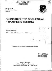
For example, if the BF10 is 4, this indicates: ‘These empirical data D are 4 times more probable if H1 were true than if H0 were true’. A BF10 between 0 and 1, in contrast, indicates support for the H0 . BFs can be calculated once for a finalized data set. But it has also repeatedly been proposed to employ BFs in sequential designs with optional stopping rules, where sample sizes are increased until a BF of a certain size has been achieved (Dienes, 2008; Kass & Raftery, 1995; Lindley, 1957; Wagenmakers et al., 2012). While unplanned optional stopping is highly problematic for NHST, it is not a problem for Bayesian statistics. For example, Edwards, Lindman, and Savage (1963) state, ‘the rules governing when data collection stops are irrelevant to data interpretation. It is entirely appropriate to collect data until a point has been proven or disproven, or until the data collector runs out of time, money, or patience’ (p. 193; see also Lindley, 1957).4 Although many authors agree about the theoretical advantages of BFs, until recently it was complicated and unclear how to compute a BF even for the simplest standard designs (Rouder, Morey, Speckman, & Province, 2012). Fortunately, over the last years BFs for several standard designs have been developed (e.g., Dienes, 2014; Gönen, Johnson, Lu, & Westfall, 2005; Kuiper, Klugkist, & Hoijtink, 2010; Morey & Rouder, 2011; Mulder, Hoijtink, & de Leeuw, 2012; Rouder et al., 2012, 2009). In the current simulations, we use the default Bayes factor proposed by Rouder et al. (2009). This BF tests H0 : m1 = m2 against H1 : δ ∼ Cauchy(r), where r is a scale parameter that controls the width of the Cauchy 5 distribution. This prior distribution defines the plausibility of possible effect sizes under H1 (more details below). The SBF procedure can be outlined as following: 1. Define a priori a threshold which indicates the requested decisiveness of evidence, for example a BF10 of 10 for H1 and the reciprocal value of 1/10 for H0 (e.g., ‘When data indicate that data are 10 times more likely under the H1 than under H0 , or vice versa, I stop sampling.’). Henceforward, these thresholds are referred to as ‘H0 boundary’ and ‘H1 boundary’.

5

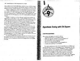
2. Choose a prior distribution for the effect sizes under H1 . This distribution describes the plausibility that effects of certain sizes exist. 3. Optionally, for confirmatory research: Pre-register the study along with the predefined threshold and prior effect size distribution. 4. Run a minimal number of participants (e.g., nmin = 20 per group), increase sample size as often as desired and compute a BF at each stage (even after each participant). 5. As soon as one of the thresholds defined in step 1 is reached or exceeded (either the H0 boundary or the H1 boundary), stop sampling and report the final BF. As a Bayesian effect size estimate, report the mean and the highest posterior density (HPD) interval of the posterior distribution of the effect size estimate, or plot the entire posterior distribution. Figure 1 shows some exemplary trajectories of how a BF10 could evolve with increasing sample size. The true effect size was δ = 0.4, and the threshold was set to 30, resp. 1/30. Selecting a threshold. As a guideline, verbal labels for BFs (‘grades of evidence’; Jeffreys, 1961, p. 432) have been suggested (Jeffreys, 1961, Kass & Raftery, 1995; see also Lee & Wagenmakers, 2013). If 1 < BF < 3, the BF indicates anecdotal evidence, 3 < BF < 10 moderate evidence, 10 < BF < 30 strong evidence, and BF > 30 very strong evidence. (Kass & Raftery, 1995, suggest 20 as threshold for ‘strong evidence’). Selecting an effect size prior for H1 . For the calculation of the BF prior distributions must be specified, which quantify the plausibility of parameter values. In the default BF for t tests (Morey & Rouder, 2011, 2015; Rouder et al., 2009) which we employ here, the plausibility of effect sizes (expressed as Cohen’s d) is modeled as a Cauchy distribution, which is called a JZS prior. The spread of the distribution can be adjusted with the scale parameter r. Figure 2 shows the Cauchy distributions for the three √ √ default values provided in the BayesFactor package (r = 2/2, 1, and 2). Higher r values lead to fatter tails, which corresponds to a higher plausibility of large effect sizes under the H1 . The family of JZS priors was constructed based on general desiderata (ly_harold_inpress; e.g., Bayarri, Berger, Forte, & García-Donato, 2012; Jeffreys, 1961), without recourse to substantive knowledge about the specifics of the problem at hand, and in this sense it is an objective prior (Rouder et al., 4 Recently, it has been debated whether BF are also biased by optional stopping rules (Sanborn & Hills, 2013; Yu et al., 2013). For a rebuttal of these positions, see Rouder (2014), and also the reply by Sanborn et al. (2014). 5 The Cauchy distribution is a t-distribution with one degree of freedom.

6

SCHÖNBRODT

Very strong H1

30

●

●●●● ●● ● ● ●

● ●● ●●

●

●

● ●

●●

● ●

Bayes Factor

Strong H1

10 Moderate H1

3 Anectodal H1

1 Anectodal H0

1/3 Moderate H0

1/10 Strong H0

1/30 Very strong H0

0

50

100

150

200

250

300

350

400

n Figure 1. Exemplary trajectories of the BF10 for a two-group mean difference with a true effect size of δ = 0.4 and scale parameter r = 1. The density curve on the top shows the distribution of sample sizes at the termination point at BF10 >= 30.

Density

0.0

0.1

0.2

0.3

0.4

r = sqrt(2)/2 r=1 r = sqrt(2)

−4

−2

0

2

4

d

Figure 2. Cauchy distribution for the distribution of effect sizes under H1 .

2009). Consequently, the default JZS priors can be used as a non-informative reference-style analysis. However, Rouder

et al. (2009) recommend to incorporate prior knowledge if available, either by tuning the width of the Cauchy prior (see Figure 2), or by choosing a different distribution for the prior. For example, Dienes, 2014 suggests to use a (half-)normal or a bounded uniform prior distribution which is tuned to prior knowledge about the underlying parameter (see also Hoijtink, 2012, for a data-based choice of prior scales). One of the most often-heard critiques of Bayesian approaches is about the necessity to choose a prior distribution of the parameters (e.g., Simmons et al., 2011). While the prior only has a relatively modest impact on Bayesian parameter estimation (any reasonable prior is quickly overwhelmed by the data; e.g., wetzels_bayesian_inpress), it exerts a lasting influence on BFs (e.g., Sinharay & Stern, 2002). Hence, the resulting strength of evidence partly depends on the specification of the model through the choice of the prior. For this reason, Jeffreys (1961) already pointed out the inevitability of an informed choice of priors for the purpose of hypothesis testing: Different questions, formalized as different specifications of H1 , lead to different answers (see also ly_harold_inpress). However, similar and sensible questions will lead to similar and sensible answers. Furthermore, the influence of the prior is not unlimited when justifiable priors are used, and it would be deceiving to claim that any BF result can be crafted just by choosing the ‘right’ prior. For example, changing the

7

SEQUENTIAL BAYES FACTORS

Method Three research designs have been introduced (NHST-PA, GS, and SBF). If these research designs are employed on a regular basis, they have several long-term properties, of which three will be investigated: (1) the long-term rate of

30

BF10 = 11.3

Strong H1

●

10

Bayes Factor

√ √ scale parameter r from the lowest ( 2/2) to the highest ( 2) default value of the BayesFactor package maximally changes the BF by a factor of 2 (Schönbrodt, 2014). In the rare cases where one prior leads to a BF favoring H1 and another prior to favoring H0 , BFs typically are in the ‘anecdotal’ region of evidence and do not provide strong evidence for either hypothesis. Practically, we see three possibilities to tackle the impact of priors on the SBF design and to forestall objections of a skeptical audience. First, without strong prior evidence for the expected effect size, we recommend to stick to a default setting (e.g., the JZS prior with r = 1) to avoid suspicion of cherry-picking a ‘favorable’ prior. Second, one should do a sensitivity analysis, which calculates a BF for a range of priors (Kass & Raftery, 1995; Spiegelhalter & Rice, 2009). If the conclusion of the BF is invariant to reasonable changes in the prior, then the results are said to be robust. Third, one could even include a sensitivity threshold within the SBF design: Only stop, when all BFs from a predefined set of priors exceed the threshold. The example in the SBF design. Here we demonstrate how the SBF procedure would have been applied to the empirical example. (For other applications of the SBF design to real data, see Matzke et al., 2015, Wagenmakers et al., 2012.) Method and participants. We employed a Sequential Bayes Factor design, where Bayes factors (BFs) are computed repeatedly during data collection, until the BF exceeds an a priori defined grade of evidence. The minimum sample size was set to nmin = 20 in each group, and the critical BF10 for stopping the sequential sampling was set to 10 (resp. 1/10). We used the JZS default BF (Rouder et al., 2009) implemented in the BayesFactor package for R (Morey & Rouder, 2015) with a scale parameter of r = 1 for the effect size prior. We computed the BF after each new participant, and the critical upper boundary was exceeded with a sample of 32 participants in each condition. Results. The final BF10 was 11.3 in favor of H1 , providing strong support for the existence of a group difference in the expected direction (two-6: M = 1.90, SD = 1.64; three-6: M = 3.88; SD = 3.24). The evolution of the BF10 can be seen in Figure 3. As an additional sensitivity analysis, we computed the BF for the other two default priors of the BayesFactor package (r = sqrt(2)/2: BF10 = 12.1; r = sqrt(2): BF10 = 9.6). Hence, the conclusion is robust with respect to reasonable variations of the effect size prior. The mean posterior effect size in the final sample was Cohen’s d = 0.72, with a 95% highest posterior density (HPD) interval of [0.22; 1.21].

Moderate H1

3 Anectodal H1

1 Anectodal H0

1/3 20 21 22 23 24 25 26 27 28 29 30 31 32

n

Figure 3. Evolution of the Bayes factor for the comparison of the two experimental groups in the empirical example.

misleading evidence, (2) the average necessary sample size to get evidence of a certain strength, and (3) the biasedness of the effect size estimates. The following sections will introduce each property with respect to the SBF design, as well as the specific settings of the simulations. Property 1: False Positive Evidence and False Negative Evidence in the SBF Design In the asymptotic case (i.e., with large enough samples), the BF10 converges either to zero (if H0 is true) or to infinity (if an effect is present; Morey & Rouder, 2011, Rouder et al., 2012), a property called consistency (Berger, 2006). Hence, with increasing sample size every SBF will converge towards (and across) the correct boundary. However, before the asymptotic case is reached any random sample can contain misleading evidence (Royall, 2000). In the case of the SBF design this would mean that the BF hits the incorrect boundary. For example, all displayed trajectories of Figure 1 hit the correct H1 boundary, but it can be seen that one of these trajectories would have prematurely hit the wrong H0 boundary if the boundary had been set to 1/10 instead of 1/30. Consequently, wrong inference is not unique to NHST – every inference procedure can produce ‘false positives’ and ‘false negatives’: False positive evidence (FPE) happens when the H1 boundary is hit although in reality H0 is true, false negative evidence (FNE) happens when the H0 boundary is hit although in reality H1 is true. It is important to note that in the cases of misleading evidence the proper interpretation of the result has been made (although it leads to an incorrect conclusion): ‘It is the evidence itself that is misleading’ (Royall, 2004, p. 124). To be very clear: The SBF is not a ‘fusion’ of Bayesian and frequentist methods, but both can provide false positive evidence (or Type I errors) and false negative evidence (or Type II errors). A major difference of the SBF approach, compared to the NHST variants, is that the long-term rate

8

SCHÖNBRODT

of wrong inference is not controlled by the researcher. As will be shown in the results of the simulation study, an SBF design has an expected long-term rate of FPE and FNE. This long-term rate, however, depends on the chosen H1 prior, the chosen threshold, and the effect size in the population. With appropriate settings, the long-term rates of misleading evidence can be kept well below 5%, but they cannot be fixed to a certain value as in NHST. Property 2: Expected Sample Sizes At what sample size can a researcher expect to hit one of both boundaries? Even when sampled from the same population, due to sampling variation some SBF studies will stop earlier and some later (see Figure 1). Hence, in contrast to NHST-PA, the final sample size is not predetermined in an SBF design. But it is possible to look at the distribution of stopping-ns and to derive the average sample number (ASN) or quantiles from it. The stopping-n distribution depends on the chosen H1 effect size prior, the chosen threshold, and the effect size in the population. Property 3: Biasedness of Effect Size Estimates Any random process can produce inaccurate individual estimates which over- or underestimate the population value. From a frequentist perspective this is not so much a problem as long as the average of all individual deviations from the true value is (close to) zero. Then the estimator is said to be unbiased. In a fixed-n design, Cohen’s dunbiased = d(1−(3/(4 df −1))) yields an unbiased estimator for the population ES (Borenstein, Hedges, Higgins, & Rothstein, 2011). If optional stopping rules depending on the effect size are introduced in a sequential design, however, things get more complicated. The design goal for GS designs, for example, is the control of Type I errors, not an unbiased estimation of the effect. For these designs it is well-known that a naive calculation of effect sizes at the termination point will overestimate the true effect for studies that are stopped early for efficacy (Emerson, Kittelson, & Gillen, 2007; Proschan et al., 2006; Whitehead, 1986; Zhang et al., 2012). When judging the bias of a sequential procedure, however, it is important to consider all studies, not just the early terminations (Goodman, 2007). When all studies are considered (i.e., early and late terminations), the bias in GS designs is only small (Fan, DeMets, & Lan, 2004; Schou & Marschner, 2013). For the assessment of the bias in an SBF design, we used the mean of the posterior effect size distribution as a Bayesian effect size estimate. Furthermore, we consider both an unconditional perspective, where the bias is investigated across all SBF studies, and a conditional perspective, where the bias is investigated conditional on early or late termination.

Settings of the Simulation For our simulation we focus on one specific scenario of hypothesis testing: the test for mean differences between two independent groups. In the NHST tradition this is usually done by a t test. As this test arguably is (one of) the most frequently employed tests in psychology, we decided to assess the properties of the SBF design based on this scenario as a first step. For simulating the two-sample mean differences, two populations (N = 1,000,000) with a normal distribution, a standard deviation of 1, and several mean differences were simulated. Random samples with increasing sample sizes were drawn from these populations (group sizes always were equal in both groups), starting from nmin = 20 for each group, and increasing the sample size in each group, until the BF exceeded the strongest boundary of 30, resp. 1/30, or nmax was reached.6 A BF for the mean difference was computed using the BayesFactor package (Morey & Rouder, 2015), with a JZS effect size prior under H1 . The following experimental conditions were varied systematically in the simulations: • The population mean difference was varied corresponding to the standardized mean difference δ = 0, 0.10, 0.20, 0.30, ..., 1.40, and 1.50. • The scale parameter r for the JZS H1 effect size prior was varied along the √ of the BayesFac√ default settings tor package: r = 2/2, 1, and 2. These values correspond to the expectation of small, medium, or large effects. • After data simulation, the trajectory of each simulated study was analyzed with regard to the stopping-n, at which each trajectory hits one of both boundaries. The boundaries were set to 3, 4, 5, 6, 7, ..., 28, 29, and 30, and their respective reciprocal values. In this simulation we only used symmetric boundaries. Henceforward, when we mention a boundary of, say, 10, this implies that the lower boundary was set to the reciprocal value of 1/10. At each boundary hit, the Bayesian effect size estimate was computed as the mean of the effect size posterior along with the 95% HPD interval (see Appendix B). In each experimental condition, 50,000 replications were simulated. When we discuss the results, we will refer to the typical situation in psychology. What effect size can be expected in 6

nmax was set to 45,000 in our simulations. In order to keep simulation time manageable, we increased the sample in several step sizes: +1 participant until n = 100, +5 participants until n = 1000, +10 participants until n = 2500, +20 participants until n = 5000, and +50 participants from that point on. In the δ=0 condition, 0.12% of trajectories did not hit one of the boundaries before nmax was reached.

SEQUENTIAL BAYES FACTORS

psychology if no prior knowledge is available? Large scale meta-meta-analyses showed that the average published effect size is around 0.5 (Bakker et al., 2012), and only 5% of published effects are larger than 1.15 (Richard, Bond, & StokesZoota, 2003). Hence, we discuss δ = 0.5 as the typical scenario in psychology. Results In the simulations, we varied true effects and boundaries on a fine-grained level. In the tables of the results section, we only present a selection of the parameter space. The full results can be seen in the Supplementary Material, and reproducible analysis scripts are available at the Open Science Framework (https://osf.io/qny5x/). Property 1: Long-term Rates of False Positive and False Negative Evidence Table 1 summarizes the long-term rates of FPE and FNE for the SBF design, which indicate how often one can expect to end up with misleading evidence. While the long-term rate of FNE quickly approaches zero with more extreme boundaries, there is a low but persistent long-term rate of FPE. As the BF converges towards and across the correct boundary, most incorrect boundary hits occur at small sample sizes. For example, at r = 1 and a boundary of 6, there is a FPE rate of 4.7%. 50% of this FPE occurs at early stopping studies with n = 1.2, the GS de-

SCHÖNBRODT

10

205 105 54

5.6 0.2 0.0 0.0 0.0 0.0 0.0 0.0 0.0

4.3 3.4 2.6

331 191 113 73 52 40 32 25 22

407 192 108 70 50 39 32 25 22

435 225 115

5.3 0.2 0.0 0.0 0.0 0.0 0.0 0.0 0.0

0.3 0.0 0.0 0.0 0.0 0.0 0.0 0.0 0.0

0.0 0.0 0.0 0.0 0.0 0.0 0.0 0.0 0.0

2.4 2.0 1.6

545 252 140 89 62 47 37 27 23

552 239 133 85 60 45 36 27 23

526 228 128 82 58 45 36 27 23

1825 927 472

0.2 0.0 0.0 0.0 0.0 0.0 0.0 0.0 0.0

0.0 0.0 0.0 0.0 0.0 0.0 0.0 0.0 0.0

0.0 0.0 0.0 0.0 0.0 0.0 0.0 0.0 0.0

1.7 1.4 1.1

636 273 151 96 67 50 40 29 24

603 260 144 92 65 49 39 28 23

571 248 139 89 63 48 39 28 23

4057 2107 1070

Table 1 Percentages of wrong inference and average sample number (ASN) for the SBF design. BF = 6 % err ASN 5.5 4.3 3.2

269 162 97 64 46 36 30 24 22

22.7 3.9 0.3 0.0 0.0 0.0 0.0 0.0 0.0

211 160 110 75 54 41 33 25 22

BF = 30 % err ASN

146 75 39

24.1 4.4 0.4 0.0 0.0 0.0 0.0 0.0 0.0

167 132 93 65 48 37 31 24 22

49.3 19.5 5.7 1.2 0.2 0.0 0.0 0.0 0.0

BF = 20 % err ASN

6.0 4.7 3.3

203 140 91 61 45 35 29 24 21 50.4 20.7 6.4 1.4 0.3 0.0 0.0 0.0 0.0

89 87 73 59 46 38 31 24 22

BF = 10 % err ASN

35.9 10.4 1.9 0.2 0.0 0.0 0.0 0.0 0.0 114 102 79 59 45 36 30 24 21

72.3 46.0 25.2 11.6 4.6 1.4 0.4 0.0 0.0

BF = 7 % err ASN

61.4 32.0 13.7 4.6 1.3 0.3 0.0 0.0 0.0

59 62 56 49 41 35 30 24 22

BF = 5 % err ASN

r/Effect size

79.1 57.3 36.9 20.8 10.4 4.7 1.8 0.2 0.0

BF = 3 % err ASN

δ = 0√ (% err relates to false positive evidence) r = 2/2 7.5 30 6.6 96 r = 1√ 5.6 24 5.1 50 4.2 22 3.4 30 r= 2 δ > 0√ (% err relates to false negative evidence) r = 2/2 δ = 0.20 77.9 34 50.6 133 δ = 0.30 60.9 36 21.7 108 δ = 0.40 42.8 35 7.0 79 δ = 0.50 26.8 33 1.7 57 δ = 0.60 15.2 30 0.3 42 δ = 0.70 7.9 27 0.0 34 δ = 0.80 3.7 25 0.0 28 δ = 1.00 0.6 22 0.0 23 δ = 1.20 0.1 21 0.0 21 r=1 δ = 0.20 84.5 27 71.5 71 δ = 0.30 71.8 28 46.6 70 δ = 0.40 56.4 29 26.2 61 δ = 0.50 40.0 28 12.4 50 δ = 0.60 26.5 27 5.2 41 δ = 0.70 15.7 26 1.7 34 δ = 0.80 8.4 24 0.5 29 δ = 1.00 1.8 22 0.0 23 δ =√1.20 0.3 21 0.0 21 r= 2 δ = 0.20 88.6 24 83.9 39 δ = 0.30 78.9 25 67.1 43 δ = 0.40 65.7 26 48.5 42 δ = 0.50 50.2 26 31.1 40 δ = 0.60 35.8 26 18.4 36 δ = 0.70 23.3 25 9.9 32 δ = 0.80 13.8 24 4.8 28 δ = 1.00 3.6 22 0.8 23 δ = 1.20 0.7 21 0.1 21

Note. δ = population effect size. r = scale parameter of H1 JZS prior. ASN = average sample number in each group.

11

SEQUENTIAL BAYES FACTORS

r = sqrt(2)/2

r=1

r = sqrt(2)

75% d = 0.2

50% 25% 0% 75%

d = 0.4

25% 0% 75%

d = 0.6

50% 25% 0%

SBF

75%

GS d = 0.8

50% 25% 0% 75%

d=1

% efficiency gain compared to NHST−PA

50%

50% 25% 0% 75%

d = 1.2

50% 25% 0% 3 6

10

20

30 3 6

10

20

30 3 6

10

20

30

Boundary Figure 4. Efficiency gain of SBF and GS designs (4 looks) compared to a fixed-n design with the same long-term rate of wrong inference. A value of 75% means that the average sample size is 75% smaller than the optimal NHST-PA fixed-n. sign seems to be on par or even more efficient than the SBF. This, however, is an artifact. The ASN of the GS design falls below 20, but nmin for the SBF design was set to 20 in our simulations. If nmin is set to 10, the SBF again is more efficient than the GS design. Property 3: Biasedness of Effect Size Estimates For each simulated study, we computed the mean of the effect size posterior as a Bayesian effect size estimate. Figure 5 focuses on a specific condition of the simulations (δ = 0.6, boundary = 4, and r = 1) and shows several perspectives on the 50,000 simulated SBF studies in that condition. Panel

A shows the distribution of effect sizes across all studies. In a fixed-n design, this distribution is a symmetric normalshaped distribution centered around the true effect size. The optional stopping of the SBF design reshapes the distribution of empirical effect sizes to a bimodal distribution: The left peak of the distribution are all studies that hit the H0 boundary (i.e., false negative evidence), the right peak are all studies that hit the H1 boundary (i.e., true positive evidence). All studies which terminated at the H0 boundary underestimated the true effect, and the majority of studies which terminated at the H1 boundary overestimated the true effect. The specific shape of the effect size distribution depends

12

SCHÖNBRODT

on the prior, the boundary separation, and the true effect size. For example, at high effect sizes and/or conservative boundaries, the FNE rate goes towards zero and consequently the left peak disappears. The unconditional meta-analytic perspective. A naive pooling of SBF studies with equal weights would ignore the fact that early stops have a smaller sample size, and therefore a smaller precision, than later stops (Goodman, 2007; Schou & Marschner, 2013; Senn, 2014). This variation in precision should be taken into account, and when the resulting effect sizes and their sample sizes are submitted to a proper meta-analysis, the estimates are slightly underestimated (see Panel B)7 . Depending on the effect size, the posterior mean underestimates the true effect by 5 to 9%. For the typical case of δ = 0.50, for example, the meta-analytic estimate would be 0.47. Hence, averaged across all studies, the Bayesian effect size estimate shows a slight downward bias. The conditional perspective. Panel C of Figure 5 shows the distribution of empirical effect sizes conditional on the stopping-n. The first subpanel, for example, shows the distribution for all studies that directly terminated at n=20. If the H1 boundary is hit very early, the effect size point estimate overestimates quite strongly. But we also mention that in early hits the posterior distribution is relatively wide, which suggests to interpret the point estimate with caution anyway. The late H1 boundary hits (see second row of Panel C), in contrast, underestimate the true effect size. This happens because just these trajectories which have a randomly low effect size in the sample take longer to accumulate the existing evidence for H1 . Hence, from a conditional perspective (i.e., conditional upon early or late termination), the SBF effect size estimate can show a bias in both directions. Practical Recommendations The following sections summarize the practical steps that are necessary to compute a sequential BF, and give some recommendations for setting boundaries and prior scales in the case of two-group t-tests. How to Compute a Sequential Bayes Factor A BF can easily be computed by online calculators8 , the BayesFactor package (Morey & Rouder, 2015) for the R Statistical Environment (R Core Team, 2014), or by the open source software JASP (Love et al., 2015). With the BayesFactor package, for example, a BF can be calculated for many common designs (e.g., one-sample designs, multiple linear regression, ANOVA designs, contingency tables, proportions). For the computation of the Bayesian effect size estimates and the 95% HPD interval, we recommend the BayesFactor package or JASP (See Appendix B for an example how to compute these in R). The ‘sequential’ part simply means that researchers can compute the BF as often

as they want – even after each single participant – and stop when the BF exceeds one of the a priori defined boundaries. Recommended Settings for Effect Size Prior and Boundary in the Two-Group t-Test If a researcher wants to employ the SBF design, the boundaries and priors have to be chosen in advance. The boundaries and the priors have an inherent meaning themselves, which should be respected. Beyond that, researchers can use the expected long-term rates for misleading evidence and the expected sample sizes as additional information for an informed choice of sensible boundaries and priors. Based on the results of the simulations, we can sketch some general recommendations for testing mean differences between two groups. First, concerning the effect size prior distribution, we recommend to set the scale parameter r to 1 as suggested by Rouder et al. (2009), unless there is a compelling reason to do otherwise. Smaller values of r increase the rate of FPE and make it rather difficult to reach the H0 boundary with a reasonable sample size (see Table 1). Furthermore, after reaching a boundary it might be compelling to perform a sensitivity analysis over reasonable r scale parameters to show that the results are robust to the choice of the prior. Second, we recommend to define a boundary of at least 5, because under typical conditions only then FPE and FNE rates tend to be low. In fact, we can hardly imagine a reasonable scenario that warrants a boundary of 3 in a sequential design, because the long-term rate for misleading evidence simply is too high. Although that reflects the current situation in psychological studies, which have an average Type II error rate of 65% (Bakker et al., 2012), the detrimental consequences of low power are well documented (e.g., Colquhoun, 2014). Third, most misleading evidence and the largest conditional bias of the estimated effect size happens at early terminations. Both can be reduced when a minimum sample is collected before the optional stopping rule is activated. Under typical conditions we recommend to collect at least 20 participants per group. Beyond these general guidelines, we want to suggest plausible choices for prototypical scenarios where the mean between two groups is compared. A reasonable setting for early lines of research could a boundary of 6 and a scale parameter of r = 1. Given a typical effect size of δ = 0.5, this setting has balanced FPE and FNE rates (4.7% and 4.6%) and has on average 46% smaller samples than optimal NHST-PA with the same error rates. In mature lines of research, confirmatory 7

We used the metafor package (Viechtbauer, 2010) and computed fixed-effect models. 8 http://pcl.missouri.edu/bayesfactor, http://www.lifesci.sussex. ac.uk/home/Zoltan_Dienes/inference/Bayes.htm

13

SEQUENTIAL BAYES FACTORS

A

B ●

Meta−analytic ES estimate

True effect size

1.5

Density

Effect size distribution of all simulated studies

1.0

0.5

0.0

1.00 ●

0.75 ●

0.50

0.6

1.0

● ● ●

0.25 ●

0.00 0.0

● ●

1.5

●

0.00

0.25

Empirical effect size estimate

0.50

0.75

1.00

1.25

True effect size

C n = 20

2

n: (20,40]

n: (40,60]

4

True effect size

3

H₁ boundary hits

H₀ boundary hits

2

6

1

3

Density

1 0

0 n: (60,80]

0 n: (80,100]

25

20

n: (100,120] 20

20

15

15

15

10 5 0

10

10

5

5

0 0

1

2

9

0 0

1

2

0

1

2

Empirical effect size estimate

Figure 5. Distribution of empirical Bayesian effect sizes in one of the experimental conditions. Distributions are based on 50,000 simulated SBF studies with δ = 0.6, r = 1, and a boundary of 4. A) The combined distribution of Bayesian effect sizes across all stopping-ns. B) Meta-analytic estimate of empirical Bayesian effect sizes for several true effect sizes, r = 1, and a boundary of 4. Other boundaries and r settings look virtually identical. C) Distribution of empirical Bayesian effect sizes conditional on the stopping-n. Panels show the effect size distributions for all studies that stopped with n directly at 20, between 20 and 40, 40 and 60, etc. True effect size is indicated by the vertical dashed line. studies may seek to gather more compelling evidence for the presence or absence of an effect. Here, the boundary should be set at least to 10. This almost guarantees to detect an existing effect (for example, for δ = 0.5 the rate of FNE is < 0.1%). If the BF does not reach such a strong boundary within practical limits (e.g., one has to stop data collection because of running out of money), one can still interpret the final BF of, say, 8 as ‘moderate evidence’. We want to emphasize again that the simulations and recommendations given here only apply to the two-tailed, twogroup t test. BFs for other designs (e.g., for multiple regression) have different prior specifications, which might have a different impact on the expected sample size and long-term

rate of misleading evidence. Furthermore, if prior knowledge is available, this should be incorporated in the settings of the SBF study. Discussion We investigated Sequential Bayes Factors (SBF) as an alternative strategy for hypothesis testing. By means of simulations we explored three properties of such a hypothesis testing strategy and compared it to an optimal NHST strategy and a group sequential design in the scenario of testing a mean difference between two groups. In the following sections we will discuss the advantages and drawbacks of the

14

SCHÖNBRODT

SBF design, and compare the hypothesis testing approach of the current paper with recent calls for a focus on accuracy in parameter estimation. Advantages of the SBF Design, Compared to NHST-PA and GS Designs Based on theoretical accounts and on the simulation results, several advantages of the SBF can be identified compared to the classical NHST-PA approach. First, with SBF (as with BF in general) it is possible to provide evidence for the H0 (Kass & Raftery, 1995). Conventional significance tests from the NHST paradigm, in contrast, do not allow to state evidence for the null. This has important implications for our understanding of science in general. According to Popper (1935, 1963) the defining property of science (in contrast to pseudo-science) is the falsifiability of theories. But, without a tool to accept the H0 , how could we ever falsify a theory that predicts an effect? If only NHST is used as our scientific tool, this would limit us to the possibility to falsify a predicted null effect, and we could not scrutinize our theories in the critical way Popper suggested (see also Gallistel, 2009). With the SBF support for the H0 is possible and we could finally bury some undead theories (Ferguson & Heene, 2012). Second, it has been shown that the SBF design necessarily converges to zero or infinity (Berger, 2006; Morey & Rouder, 2011; Rouder et al., 2012). The goal for planning a study, for example via a priori power analyses, is to avoid inconclusive evidence. With an SBF design, the long-term rate of weak evidence can be pushed to zero and no study will end up with an inconclusive result, as long as researchers don’t run out of participants. Third, the BF provides a continuous measure of evidence. But does the SBF revive the black-and-white-dichotomy of the NHST, which we seek to overcome? No. The ‘sequential’ part of the SBF does include a binary decision: Should I continue sampling, or should I stop? But this dichotomy should not be mixed up with the binary decision, ‘Is there an effect, or not?’. The BF is a continuous measure that tells researchers how to update their prior beliefs about H0 and H1 , and it stays continuous in the SBF design. Furthermore, nothing prevents the researcher to continue sampling after a first threshold is reached, or to stop before a threshold is reached – these sampling decisions do not change the meaning of the resulting BF (Rouder, 2014). It is important to emphasize that, in contrast to NHST, the SBF stopping rule is more a suggestion, not a prescription. The presented simulations show what sample sizes and long-term rates of misleading evidence a researcher can expect if s/he sticks to the stopping rule. Hence, the predefined threshold is only necessary to compute the expected properties of the SBF method. From a Bayesian point of view, the boundaries are not necessary and a researcher can keep on collecting data until he

or she ‘runs out of time, money, or patience’ (Edwards et al., 1963, p. 163). Fourth, one can make interim tests as often as wanted, without engaging in a questionable research practice. When the data are inconclusive, simply increase sample size until they are. This property of the SBF also corresponds to the intuition of many researchers, as has been expressed by Edwards et al. (1963): ‘This irrelevance of stopping rules to statistical inference restores a simplicity and freedom to experimental design that had been lost by classical emphasis on significance levels’ (p. 239). Fifth, the SBF is about 50 - 70% more efficient than the optimal NHST design, and even more efficient than a typical GS design. Optional stopping procedures give the opportunity to stop early when the effect is strong, and to continue sampling when the effect is weaker than expected. Finally, compared to GS or adaptive designs in the NHST tradition, the SBF design is easier to implement and more flexible. It is convenient to compute BFs using one of the websites, JASP, or the BayesFactor R package. There is no need for difficult pre-planning, variance spending plans, or a priori effects size estimates. Disadvantages of the SBF and Limitations of the Simulation Beyond these clear advantages, the SBF also has potential limitations. First, even amongst Bayesians, the BF in general (e.g., Gelman & Rubin, 1995; Kruschke, 2011, 2012), or its specific formulations (e.g., Johnson, 2013) are not without criticism. Even amongst proponents of the BF, there is no general consensus yet about what types of priors should be used in which situations. Here, we focus on a default JZS BF for t tests, as proposed by Morey and Rouder (2011) and Rouder et al. (2009), but there are other ways to compute BFs, which, for example, incorporate prior knowledge about the research topic (Dienes, 2014). Second, SBF as we defined it here, is an open procedure with an unbounded sample size. GS designs, in contrast, still have an upper limit of sample size which is known in advance (Jennison & Turnbull, 1999). If the true effect size is close to zero (but not zero), it could happen that a SBF meanders for thousands of participants in the ‘undecided’ region before it finally drifts towards the H1 boundary. This property can make studies hard to plan, which could be problematic for funding agencies that expect a precise planning of sample size. On the other hand, researchers can still decide a priori to use a maximum sample size in a SBF design given logistical constraints and theoretical considerations. Third, not for every design exists a handy default BF procedure, at least for the moment. For example, if complicated multilevel models or structural equation models are to be tested, it is probably more convenient to work in a Bayesian estimation framework, or to fall back to fixed-n designs.

SEQUENTIAL BAYES FACTORS

Fourth, it is not possible to define the rate of FPE and FNE a priori. Table 1, Table A1, and the Supplementary Material allow to envisage expected long-term rates of misleading evidence, but proper error control is the realm of NHST. Fifth, it could be considered as a disadvantage that final effect size estimates can be biased upwards conditional on early termination, or biased downwards conditional on late termination. This is a property that the SBF shares with all sequential designs, Bayesian and non-Bayesian (Proschan et al., 2006). In the context of clinical sequential designs, substantial efforts have been undertaken to provide corrections for that conditional bias (Chuang & Lai, 2000; Emerson & Fleming, 1990; Fan et al., 2004; Li & DeMets, 1999; Liu, 2003; Pocock & Hughes, 1989; Whitehead, 1986). The issue of conditional bias correction after a sequential design, however, is less well understood than the control of Type I error rates, and remains an active topic of research. Future studies should investigate whether and how techniques for correcting the conditional bias could be applied to an SBF design. From an unconditional perspective, underestimations from late terminations balance the overestimations from early terminations (Senn, 2014), which led Schou and Marschner (2013) to conclude that ‘early stopping of clinical trials for apparent benefit is not a substantive source of bias in meta-analyses [...]. Evidence synthesis should be based on results from all studies, both truncated and non-truncated’ (p. 4873). Furthermore, they conclude that mixing sequential and fixed-n designs is not problematic. Due to the Bayesian shrinkage of early terminations, meta-analytic aggregations of multiple SBF studies underestimate the true effect size by 5-9%. This analysis, however, presumes that all studies are included in the meta-analysis – both H0 and H1 boundary hits, and both early and late terminations. We assume that publication bias favors studies that a) hit the H1 boundary, and b) stop earlier rather than later. As such a selection pressure leads to overestimated effect sizes, the slight overall underestimation can be considered a useful attenuation. Other authors have argued that beyond the issue of unbiasedness the variance of effect size estimates should be considered. The sequential procedure could increase the heterogeneity of results compared to the fixed-n case, leading to an erroneous application of a meta-analytic random effects model (Hughes, Freedman, & Pocock, 1992; see also Braschi, Botella, & Suero, 2014). But not all sequential procedures are alike, and it is unclear how simulation results from one procedure generalize to other procedures. In summary, and as emphasized before, the SBF focuses on efficient hypothesis testing, and not on unbiased and precise parameter estimates. Nonetheless, given that the bias is rather small in practical terms, we tentatively conclude that Bayesian effect size estimates from SBF studies can be included in metaanalyses. But certainly more research is needed before firm

15

conclusions can be drawn about the effects of optional stopping rules on research synthesis in general. A final limitation of the current simulations is that we only focused on the two-sample, two-sided t test. Although we only investigated one specific test, the general sequential procedure can be applied to every BF. The specific results of our simulations, such as the expected sample size, however, cannot be generalized to other tests. For example, the ASN will be much lower for within-subject designs. Hypothesis Testing vs. Accuracy in Parameter Estimation Several recent contributions aimed at shifting away from hypothesis testing towards accuracy/precision9 of parameter estimation (Cumming, 2014; Eich, 2014; Kelley & Maxwell, 2003; Maxwell et al., 2008). Morey, Rouder, Verhagen, and Wagenmakers (2014), while agreeing with many of these recommendations, have argued, however, that hypothesis tests are also essential for psychological science. Hypothesis testing and estimation sometimes answer different questions. Some question may be better answered from a hypothesis-testing point of view, some other rather from a estimation/accuracy point of view, and ‘[...] the goals of error control and accurate estimation can sometimes be in direct conflict.’ (Goodman, 2007, p. 882).10 These different goals could be captured in a trade-off between accuracy and efficiency. Accuracy focuses on obtaining parameter estimates that are unbiased and precise. Efficiency, in contrast, focuses on reliably detecting an effect as quickly as possible. If the main goal is to get accurate and stable estimates, one cannot optimize efficiency. For example, for typical effect sizes it has been shown that estimates of correlations only tend to stabilize when n is approaching 250 (Schönbrodt & Perugini, 2013), and in order to obtain accurate estimates of a group difference with the typical effect size, one needs more than 500 participants per group (Kelley & Rausch, 2006). If the focus is on efficient hypothesis testing, in contrast, an SBF design can answer the question about the presence of an effect with strong evidence after only 73 participants on average (instead of 500). When the main question of interest is the precision of the estimate, other approaches, such as ‘planning for accu9

Precision and accuracy are conceptually different concepts that are equivalent only when the expected value of a parameter is equal to the parameter value it represents. We use the term accuracy here for consistency with most previous relevant literature. However, note that if the population values are unknown, it would be safer to use the term precision. For a discussion of the relationship between accuracy and precision, see Kelley and Rausch (2006) and Ledgerwood and Shrout (2011). 10 For a discussion of the ethical consequences of estimation vs. hypothesis testing in the medical sciences, see Mueller, Montori, Bassler, Koenig, and Guyatt (2007) and Goodman (2007).

16

SCHÖNBRODT

racy’ (Kruschke, 2012; Maxwell et al., 2008), might be better suited. Hence, accuracy in an estimation framework and efficiency in a sequential hypothesis testing framework are complementary goals for different research scenarios. Conclusion In an ideal world, scientists would have precise theories, easy access to thousands of participants, and highly reliable measures. In such a scenario, any reasonable hypothesis test procedure would come to the same conclusions, and researchers would have no need to use an optional stopping rule that depends on the effect size. In a realistic scenario, however, where resources are limited and researchers have the obligation to use these resources wisely, the SBF can answer the question about the presence or absence of an effect with better quality (i.e., a smaller long-term rate of misleading evidence) and/or higher efficiency (i.e., fewer participants on average) than the classical NHST-PA approach or typical frequentist sequential designs. Furthermore, it is highly flexible concerning the sampling plan and does not depend on correct a priori guesses of the true effect size. Therefore, a prototypical scenario for the application of the SBF design could be early lines of research that sort out which effects hold promise (see also Lakens, 2014). Furthermore, its efficiency makes it especially valuable when samples are hard to collect or limited in size, such as clinical samples. After the presence of an effect is established with strong evidence, accumulating samples or meta-analyses can provide unbiased and increasingly accurate estimates of the effect size. It is important to stress that the SBF design is not a magic wand, it has both advantages and disadvantages, and it should not be used mindlessly. However, it represents a valid approach for hypothesis testing with some distinctive desirable properties that set it apart from current common alternatives. Among these, we wish to stress that it makes a commonly used procedure perfectly acceptable, which has been considered as questionable so far: If the results are unclear, collect more data. While in NHST this option is taboo, using the SBF it can be done without any guilt. Not only it can be done, but doing so results in a more efficient research strategy, provided that some rules are followed. References Anderson, K. (2014). gsDesign: Group Sequential Design. Armitage, P., McPherson, C. K., & Rowe, B. C. (1969). Repeated significance tests on accumulating data. Journal of the Royal Statistical Society. Series A (General), 132, 235–244. Bakan, D. (1966). The test of significance in psychological research. Psychological Bulletin, 66, 423–437. doi:10. 1037/h0020412

Bakker, M., van Dijk, A., & Wicherts, J. M. (2012). The rules of the game called psychological science. Perspectives on Psychological Science, 7, 543–554. doi:10 . 1177 / 1745691612459060 Bayarri, M. J., Berger, J. O., Forte, A., & García-Donato, G. (2012). Criteria for Bayesian model choice with application to variable selection. The Annals of Statistics, 40, 1550–1577. Berger, J. O. (2006). Bayes factors. In S. Kotz, N. Balakrishnan, C. Read, B. Vidakovic, & N. L. Johnson (Eds.), Encyclopedia of statistical sciences, vol. 1 (2nd ed.) (pp. 378–386). Hoboken, NJ: Wiley. Berger, J. O. & Wolpert, R. L. (1988). The likelihood principle (2nd ed.) Hayward, CA: Institute of Mathematical Statistics. Borenstein, M., Hedges, L. V., Higgins, J. P. T., & Rothstein, H. R. (2011). Introduction to meta-analysis. Chichester: John Wiley & Sons. Braschi, L., Botella, J., & Suero, M. (2014). Consequences of sequential sampling for meta-analysis. Behavior Research Methods, 46, 1167–1183. doi:10.3758/s13428013-0433-z Chambers, C. D. (2013). Registered Reports: A new publishing initiative at Cortex. Cortex, 49, 609–610. doi:10. 1016/j.cortex.2012.12.016 Chuang, C. S. & Lai, T. L. (2000). Hybrid resampling methods for confidence intervals. Statistica Sinica, 10, 1– 50. Cohen, J. (1988). Statistical power analysis for the behavioral sciences. New Jersey, US: Lawrence Erlbaum Associates. Cohen, J. (1994). The earth is round (p < .05). American Psychologist, 49, 997–1003. doi:10.1037/0003-066X.49. 12.997 Colquhoun, D. (2014). An investigation of the false discovery rate and the misinterpretation of p-values. Royal Society Open Science, 1, 140216. doi:10 . 1098 / rsos . 140216 Cumming, G. (2014). The new statistics: Why and how. Psychological Science, 25, 7–29. doi:10 . 1177 / 0956797613504966 Dienes, Z. (2008). Understanding psychology as a science: An introduction to scientific and statistical inference. New York: Palgrave Macmillan. Dienes, Z. (2011). Bayesian versus orthodox statistics: Which side are you on? Perspectives on Psychological Science, 6, 274–290. doi:10.1177/1745691611406920 Dienes, Z. (2014). Using Bayes to get the most out of nonsignificant results. Frontiers in Psychology: Quantitative Psychology and Measurement, 5, 781. doi:10 . 3389/fpsyg.2014.00781 Edwards, W., Lindman, H., & Savage, L. J. (1963). Bayesian statistical inference for psychological research. Psy-

SEQUENTIAL BAYES FACTORS

chological Review, 70, 193–242. doi:10 . 1037 / h0044139 Eich, E. (2014). Business not as usual. Psychological Science, 25, 3–6. doi:10.1177/0956797613512465 Emerson, S. S. & Fleming, T. R. (1990). Parameter estimation following group sequential hypothesis testing. Biometrika, 77, 875–892. Emerson, S. S., Kittelson, J. M., & Gillen, D. L. (2007). Frequentist evaluation of group sequential clinical trial designs. Statistics in Medicine, 26, 5047–5080. doi:10 . 1002/sim.2901 Fan, X., DeMets, D. L., & Lan, K. K. G. (2004). Conditional bias of point estimates following a group sequential test. Journal of Biopharmaceutical Statistics, 14, 505– 530. doi:10.1081/BIP-120037195 Ferguson, C. J. & Heene, M. (2012). A vast graveyard of undead theories: Publication bias and psychological science’s aversion to the null. Perspectives on Psychological Science, 7, 555–561. doi:10 . 1177 / 1745691612459059 Frick, R. W. (1998). A better stopping rule for conventional statistical tests. Behavior Research Methods, Instruments, & Computers, 30, 690–697. doi:10 . 3758 / BF03209488 Gallistel, C. R. (2009). The importance of proving the null. Psychological Review, 116, 439–453. Gelman, A. & Rubin, D. B. (1995). Avoiding model selection in Bayesian social research. Sociological Methodology, 25, 165–174. Gigerenzer, G., Krauss, S., & Vitouch, O. (2004). The null ritual. In D. Kaplan (Ed.), The Sage handbook of quantitative methodology for the social sciences (pp. 391– 408). Thousand Oaks, CA: Sage. Gönen, M., Johnson, W. O., Lu, Y., & Westfall, P. H. (2005). The Bayesian two-sample t test. The American Statistician, 59, 252–257. doi:10.1198/000313005X55233 Goodman, S. N. (2007). Stopping at nothing? Some dilemmas of data monitoring in clinical trials. Annals of Internal Medicine, 146, 882–887. Hoijtink, H. (2012). Informative hypotheses: Theory and practice for behavioral and social scientists. Boca Raton: Chapman and Hall/CRC. Hubbard, R. (2011). The widespread misinterpretation of pvalues as error probabilities. Journal of Applied Statistics, 38, 2617–2626. doi:10 . 1080 / 02664763 . 2011 . 567245 Hughes, M. D., Freedman, L. S., & Pocock, S. J. (1992). The impact of stopping rules on heterogeneity of results in overviews of clinical trials. Biometrics, 48, 41–53. Jeffreys, H. (1961). The theory of probability. Oxford University Press.

17

Jennison, C. & Turnbull, B. W. (1999). Group sequential methods with applications to clinical trials. Boca Raton: CRC Press. John, L. K., Loewenstein, G., & Prelec, D. (2012). Measuring the prevalence of questionable research practices with incentives for truth telling. Psychological Science, 23, 524–532. doi:10.1177/0956797611430953 Johnson, V. E. (2013). Revised standards for statistical evidence. Proceedings of the National Academy of Sciences, 110, 19313–19317. doi:10 . 1073 / pnas . 1313476110 Kass, R. E. & Raftery, A. E. (1995). Bayes factors. Journal of the American Statistical Association, 90, 773–795. Kelley, K. & Maxwell, S. E. (2003). Sample size for multiple regression: Obtaining regression coefficients that are accurate, not simply significant. Psychological Methods, 8, 305–321. Kelley, K. & Rausch, J. R. (2006). Sample size planning for the standardized mean difference: Accuracy in parameter estimation via narrow confidence intervals. Psychological Methods, 11, 363–385. doi:10.1037/1082989X.11.4.363 Klein, R. A., Ratliff, K. A., Vianello, M., Adams Jr., R. B., Bahník, Š., Bernstein, M. J., . . . Nosek, B. A. (2014). Investigating variation in replicability: A “many labs” replication project. Social Psychology, 45, 142–152. doi:10.1027/1864-9335/a000178 Kline, R. B. (2004). Beyond significance testing: Reforming data analysis methods in behavioral research. Washington, DC: APA. Kruschke, J. K. (2011). Bayesian assessment of null values via parameter estimation and model comparison. Perspectives on Psychological Science, 6, 299–312. doi:10.1177/1745691611406925 Kruschke, J. K. (2012). Bayesian estimation supersedes the t test. Journal of Experimental Psychology: General, 1–31. doi:10.1037/a0029146 Kuiper, R. M., Klugkist, I., & Hoijtink, H. (2010). A Fortran 90 program for confirmatory analysis of variance. Journal of Statistical Software, 34, 1–30. Lai, T. L., Lavori, P. W., & Shih, M. C. (2012). Adaptive trial designs. Annual Review of Pharmacology and Toxicology, 52, 101–110. doi:10 . 1146 / annurev - pharmtox 010611-134504 Lakens, D. (2014). Performing high-powered studies efficiently with sequential analyses. European Journal of Social Psychology, 44, 701–710. doi:10 . 1002 / ejsp . 2023 Ledgerwood, A. & Shrout, P. E. (2011). The trade-off between accuracy and precision in latent variable models of mediation processes. Journal of Personality and Social Psychology, 101, 1174–1188. doi:10 . 1037 / a0024776

18

SCHÖNBRODT

Lee, M. D. & Wagenmakers, E.-J. (2013). Bayesian cognitive modeling: A practical course. Cambridge University Press. Li, Z. & DeMets, D. L. (1999). On the bias of estimation of a Brownian motion drift following group sequential tests. Statistica Sinica, 9, 923–938. Lindley, D. V. (1957). A statistical paradox. Biometrika, 44, 187–192. doi:10.1093/biomet/44.1-2.187 Liu, A. (2003). A simple low-bias estimate following a sequential test with linear boundaries. Lecture NotesMonograph Series, 47–58. Love, J., Selker, R., Marsman, M., Jamil, T., Verhagen, J., Ly, A., . . . Wagenmakers, E.-J. (2015). JASP (Version 0.7.1). Matzke, D., Nieuwenhuis, S., van Rijn, H., Slagter, H. A., van der Molen, M. W., & Wagenmakers, E.-J. (2015). The effect of horizontal eye movements on free recall: A preregistered adversarial collaboration. Journal of Experimental Psychology. General, 144, e1–15. doi:10.1037/xge0000038 Maxwell, S. E., Kelley, K., & Rausch, J. R. (2008). Sample size planning for statistical power and accuracy in parameter estimation. Annual Review of Psychology, 59, 537–563. doi:10.1146/annurev.psych.59.103006. 093735 Morey, R. D. & Rouder, J. N. (2011). Bayes factor approaches for testing interval null hypotheses. Psychological Methods, 16, 406–419. doi:10.1037/a0024377 Morey, R. D. & Rouder, J. N. (2015). BayesFactor: Computation of Bayes factors for common designs. Morey, R. D., Rouder, J. N., Verhagen, J., & Wagenmakers, E.-J. (2014). Why hypothesis tests are essential for psychological science: A comment on Cumming (2014). Psychological Science, 0956797614525969. doi:10.1177/0956797614525969 Mueller, P. S., Montori, V. M., Bassler, D., Koenig, B. A., & Guyatt, G. H. (2007). Ethical issues in stopping randomized trials early because of apparent benefit. Annals of Internal Medicine, 146, 878–881. doi:10.7326/ 0003-4819-146-12-200706190-00009 Mulder, J., Hoijtink, H., & de Leeuw, C. (2012). BIEMS: A Fortran 90 program for calculating Bayes factors for inequality and equality constrained models. Journal of Statistical Software, 46, 1–39. Murayama, K., Pekrun, R., & Fiedler, K. (2013). Research practices that can prevent an inflation of falsepositive rates. Personality and Social Psychology Review. doi:10.1177/1088868313496330 Nosek, B. A. & Lakens, D. (2014). Registered reports: A method to increase the credibility of published results. Social Psychology, 45, 137–141. doi:10 . 1027 / 1864 9335/a000192

Oppenheimer, D. M. & Monin, B. (2009). The retrospective gambler’s fallacy: Unlikely events, constructing the past, and multiple universes. Judgment and Decision Making, 4, 326–334. Perugini, M., Gallucci, M., & Costantini, G. (2014). Safeguard power as a protection against imprecise power estimates. Perspectives on Psychological Science, 9, 319–332. doi:10.1177/1745691614528519 Plummer, M., Best, N., Cowles, K., & Vines, K. (2006). CODA: Convergence diagnosis and output analysis for MCMC. R News, 6, 7–11. Pocock, S. J. & Hughes, M. D. (1989). Practical problems in interim analyses, with particular regard to estimation. Controlled Clinical Trials, 10, 209–221. Popper, K. R. (1935). Logik der Forschung. Vienna, Austria: Julius Springer. Popper, K. R. (1963). Conjectures and refutations: The growth of scientific knowledge. London: Routledge. Proschan, M. A., Lan, K. G., & Wittes, J. T. (2006). Statistical monitoring of clinical trials: A unified approach. New York: Springer. R Core Team. (2014). R: A language and environment for statistical computing. Vienna, Austria. Richard, F. D., Bond, C. F., & Stokes-Zoota, J. J. (2003). One hundred years of social psychology quantitatively described. Review of General Psychology, 7, 331–363. doi:10.1037/1089-2680.7.4.331 Rouder, J. N. (2014). Optional stopping: No problem for bayesians. Psychonomic Bulletin & Review, 21, 301– 308. doi:10.3758/s13423-014-0595-4 Rouder, J. N., Morey, R. D., Speckman, P. L., & Province, J. M. (2012). Default Bayes factors for ANOVA designs. Journal of Mathematical Psychology, 56, 356– 374. doi:10.1016/j.jmp.2012.08.001 Rouder, J. N., Speckman, P. L., Sun, D., Morey, R. D., & Iverson, G. (2009). Bayesian t tests for accepting and rejecting the null hypothesis. Psychonomic Bulletin & Review, 16, 225–237. Royall, R. M. (1997). Statistical evidence: A likelihood paradigm. London: Chapman & Hall. Royall, R. M. (2000). On the probability of observing misleading statistical evidence. Journal of the American Statistical Association, 95, 760–768. doi:10 . 2307 / 2669456 Royall, R. M. (2004). The likelihood paradigm for statistical evidence. In M. L. Taper & S. R. Lele (Eds.), The nature of scientific evidence: Statistical, philosophical, and empirical considerations (pp. 119–152). Chicago: University of Chicago Press. Rozeboom, W. W. (1960). The fallacy of the null-hypothesis significance test. Psychological Bulletin, 57, 416–428. doi:10.1037/h0042040

SEQUENTIAL BAYES FACTORS

19

Sanborn, A. N. & Hills, T. T. (2013). The frequentist impliViechtbauer, W. (2010). Conducting meta-analyses in R with cations of optional stopping on Bayesian hypothesis the metafor package. Journal of Statistical Software, tests. Psychonomic Bulletin & Review. doi:10 . 3758 / 36, 1–48. s13423-013-0518-9 Wagenmakers, E.-J. (2007). A practical solution to the perSanborn, A. N., Hills, T. T., Dougherty, M. R., Thomas, R. P., vasive problems of p values. Psychonomic Bulletin & Yu, E. C., & Sprenger, A. M. (2014). Reply to Rouder Review, 14, 779–804. (2014): Good frequentist properties raise confidence. Wagenmakers, E.-J., Wetzels, R., Borsboom, D., v. d. Maas, Psychonomic Bulletin & Review. doi:10.3758/s13423H. L. J., & Kievit, R. A. (2012). An agenda for purely 014-0607-4 confirmatory research. Perspectives on Psychological Schmidt, F. L. & Hunter, J. E. (1997). Eight common but Science, 7, 632–638. doi:10.1177/1745691612463078 false objections to the discontinuation of significance Wagenmakers, E.-J., Beek, T. F., Rotteveel, M., Gierholz, testing in the analysis of research data. In L. L. HarA., Matzke, D., Steingroever, H., . . . Pinto, Y. (2015). low, S. A. Mulaik, & J. H. Steiger (Eds.), What if there Turning the hands of time again: A purely confirmawere no significance tests? (pp. 37–64). Mahwah, New tory replication study and a Bayesian analysis. CogniJersey: Lawrence Erlbaum Associates. tion, 494. doi:10.3389/fpsyg.2015.00494 Schönbrodt, F. D. (2014). Interactive exploration of a prior’s Wald, A. & Wolfowitz, J. (1948). Optimum character of the impact (Blog post). sequential probability ratio test. The Annals of MathSchönbrodt, F. D. & Perugini, M. (2013). At what sample ematical Statistics, 19, 326–339. doi:10 . 1214 / aoms / size do correlations stabilize? Journal of Research in 1177730197 Personality, 47, 609–612. doi:10.1016/j.jrp.2013.05. Whitehead, J. (1986). On the bias of maximum likelihood 009 estimation following a sequential test. Biometrika, 73, Schou, I. M. & Marschner, I. C. (2013). Meta-analysis of 573–581. doi:10.1093/biomet/73.3.573 clinical trials with early stopping: An investigation of Yu, E. C., Sprenger, A. M., Thomas, R. P., & Dougherty, potential bias. Statistics in Medicine, 32, 4859–4874. M. R. (2013). When decision heuristics and science doi:10.1002/sim.5893 collide. Psychonomic Bulletin & Review. doi:10.3758/ Senn, S. (2014). A note regarding meta-analysis of sequens13423-013-0495-z tial trials with stopping for efficacy. Pharmaceutical Zhang, J. J., Blumenthal, G. M., He, K., Tang, S., Cortazar, Statistics, 13, 371–375. doi:10.1002/pst.1639 P., & Sridhara, R. (2012). Overestimation of the efSimmons, J. P., Nelson, L. D., & Simonsohn, U. (2011). fect size in group sequential trials. Clinical Cancer ReFalse-positive psychology: Undisclosed flexibility in search, 18, 4872–4876. doi:10.1158/1078-0432.CCRdata collection and analysis allows presenting anything 11-3118 as significant. Psychological Science, 22, 1359–1366. doi:10.1177/0956797611417632 Appendix A Simonsohn, U. (2013). Just post it: The lesson from two Quantiles for Stopping-ns cases of fabricated data detected by statistics alone. While Table 1 reports the average sample size until a SBF dePsychological Science, 24, 1875–1888. doi:10.1177/ sign can be stopped (ASN), this table reports the quantiles of 0956797613480366 each stopping-n distribution. The four numbers in each cell Simonsohn, U., Nelson, L. D., & Simmons, J. P. (2014). Pare the 50th, 80th, 90th, and 95th quantile of the respective curve: A key to the file-drawer. Journal of Experimenstopping-n distribution. tal Psychology: General, 143, 534–547. doi:10.1037/ a0033242 Appendix B Sinharay, S. & Stern, H. S. (2002). On the sensitivity of How to Compute the Bayesian Effect Size Estimate With HPD Interval Bayes factors to the prior distributions. The American Using the BayesFactor (Morey & Rouder, 2015) and the Statistician, 56, 196–201. coda package (Plummer, Best, Cowles, & Vines, 2006) for Spiegelhalter, D. & Rice, K. (2009). Bayesian statistics. R, both Bayes factors and Bayesian effect size estimates can Scholarpedia, 4, 5230. doi:10.4249/scholarpedia.5230 be easily computed: van Assen, M. A. L. M., van Aert, R. C. M., Nuijten, M. B., & Wicherts, J. M. (2014). Why publishing everything is ## lines beginning with # are comments more effective than selective publishing of statistically significant results. PLoS ONE, 9, e84896. doi:10.1371/ # if not already done: journal.pone.0084896 # install the BayesFactor package # (only has to be done once) # install.packages("BayesFactor")

SCHÖNBRODT

20

23/42/68/110 25/53/84/130 27/57/83/115 29/54/73/92 27/47/61/75 25/41/51/62 22/34/43/51 20/25/31/36 20/20/23/27

40/82/145/225 44/95/150/200 45/85/120/150 39/70/92/115 33/56/71/86 27/45/57/68 22/36/45/54 20/24/30/36 20/20/22/26

80/190/290/395 79/165/220/275 64/120/155/190 45/82/110/130 33/59/77/93 26/45/58/70 22/35/45/54 20/24/30/35 20/20/22/26

69/110/160/220 36/56/79/115 21/32/45/62

BF = 5

30/64/120/200 35/83/140/195 38/80/115/150 37/69/92/115 33/57/73/88 28/47/59/70 24/38/48/56 20/26/32/38 20/20/24/28

61/155/260/375 69/155/215/275 62/120/155/190 48/86/115/135 37/63/81/98 28/48/62/74 23/38/48/57 20/25/31/37 20/20/23/27

135/305/440/565 115/215/280/340 74/140/180/215 49/89/120/145 36/63/81/98 28/47/60/73 23/37/46/56 20/25/31/36 20/20/23/27

105/170/245/340 53/83/125/175 28/44/63/88

BF = 6

43/110/205/320 52/130/195/260 53/110/150/185 47/84/110/135 38/65/83/99 31/51/65/77 25/40/51/61 20/27/33/39 20/21/24/29

92/250/385/525 96/200/270/335 75/140/180/220 54/95/125/150 38/67/87/105 30/50/64/78 24/39/49/59 20/26/32/38 20/20/24/28

200/415/565/695 135/250/320/390 79/150/195/235 51/93/125/150 37/65/84/105 29/49/62/75 24/38/48/58 20/26/32/38 20/20/24/28

150/235/335/475 73/120/175/250 38/60/86/130

BF = 7

115/335/510/665 125/245/325/395 90/165/210/250 63/115/145/170 45/77/98/120 34/57/72/86 27/44/55/66 20/29/36/42 20/22/26/30

255/515/685/835 165/295/372/445 93/175/220/260 60/110/140/170 43/74/94/115 33/55/69/83 26/42/53/63 20/28/35/41 20/21/25/30

350/625/795/955 165/300/385/460 88/165/210/255 58/105/135/160 42/71/91/110 32/53/67/81 26/42/52/62 20/28/34/40 20/21/25/29

305/490/710/1020 160/255/365/526 77/130/190/280

BF = 10

485/815/1020/1200 225/380/470/555 125/210/260/305 76/130/165/195 53/88/115/135 40/65/81/96 31/50/62/73 22/33/40/47 20/24/29/34

495/835/1050/1230 210/360/455/535 115/200/250/295 72/125/160/190 51/85/110/130 39/63/79/93 31/49/60/71 22/32/39/46 20/24/29/33

465/795/1010/1190 200/345/435/515 110/190/240/285 70/120/155/180 50/82/105/125 38/62/77/91 30/48/59/69 22/32/39/46 20/24/28/33

1250/1990/2960/4440 625/1000/1500/2200 320/520/765/1130

BF = 20

580/940/1160/1360 250/405/500/585 135/225/275/325 83/140/175/205 58/95/120/140 43/70/87/105 34/54/66/78 23/35/43/50 20/26/31/36

545/900/1120/1310 235/390/480/565 130/215/265/310 80/135/170/200 56/91/115/135 42/68/84/99 33/52/64/76 23/35/42/49 20/25/30/35

510/855/1070/1260 220/370/465/545 125/205/255/300 77/130/165/190 55/89/115/135 42/66/82/96 33/52/63/74 23/34/42/49 20/25/30/35

2820/4560/6900/10100 1420/2290/3440/5200 710/1150/1710/2560

BF = 30

Table A1 Expected stopping-n for SBF designs: Quantiles BF = 3 Stopping-n at δ = 0 √ r = 2/2 22/34/45/60 r=1 20/25/32/40 √ 20/21/26/32 r= 2 Stopping-n at δ > 0 √ r = 2/2 δ = 0.20 24/39/56/77 δ = 0.30 25/44/63/84 δ = 0.40 26/45/61/78 δ = 0.50 25/42/56/69 δ = 0.60 23/38/49/59 δ = 0.70 21/33/42/50 δ = 0.80 20/28/35/42 δ = 1.00 20/21/26/30 δ = 1.20 20/20/20/23 r=1 δ = 0.20 20/28/38/51 δ = 0.30 20/32/44/58 δ = 0.40 21/34/45/58 δ = 0.50 21/34/44/55 δ = 0.60 21/32/41/50 δ = 0.70 21/30/37/45 δ = 0.80 20/27/33/39 δ = 1.00 20/21/26/30 δ =√1.20 20/20/21/23 r= 2 δ = 0.20 20/23/30/39 δ = 0.30 20/26/35/45 δ = 0.40 20/28/37/47 δ = 0.50 20/29/38/46 δ = 0.60 20/29/37/44 δ = 0.70 20/28/35/41 δ = 0.80 20/26/32/37 δ = 1.00 20/22/26/30 δ = 1.20 20/20/21/24

Note. r = scale parameter of H1 prior. δ = true effect size. Numbers in each cell are the 50th, 80th, 90th, and 95th quantile of each stopping-n distribution. Stopping-n is sample size in each group.

SEQUENTIAL BAYES FACTORS

# load the package for the active session library(BayesFactor) # open the help page ?ttestBF # load a built-in data set data(sleep) ## ## ## BF

Compute the Bayes factor for a two-group mean comparison. Set r to 1 It's very weak evidence (BF=1.15) # --> for a group difference

## Compute the Bayesian effect size estimate samples Bayesian ES estimate = -0.6794 (see "delta") # --> 95% HPD interval [-1.54; 0.15]