tapping rate of musical audio signals [1],[2]. However these approaches do not distinguish between tempo and rhythm. Goto and Muraoka detail a system which ...
SEQUENTIAL INFERENCE OF RHYTHMIC STRUCTURE IN MUSICAL AUDIO Nick Whiteley
A. Taylan Cemgil
Simon Godsill
University of Cambridge Department of Engineering Signal Processing and Communications Laboratory ABSTRACT This paper presents a framework for the modelling of temporal characteristics of musical signals and an approximate, sequential Monte Carlo inference scheme which yields estimates of tempo and rhythmic pattern from onset-time data. These two features are quanti¿ed through the construction of a probabilistic dynamical model of a hidden ‘bar-pointer’ and a Poisson observation model. The capabilities of the system are demonstrated by tracking the tempo of a 2 against 3 polyrhythm and detecting a switch in rhythm in a MIDI performance. Index Terms— Music, Statistics, Poisson distributions, Monte Carlo methods 1. INTRODUCTION An important feature of intelligent music systems is the ability to infer attributes related to temporal structure. These attributes may include musicological constructs such as tempo and rhythmic pattern. The recognition of these characteristics forms a sub-task of automatic music transcription - the unsupervised generation of a score, or description of an audio signal in terms of musical concepts. For music categorization systems, tempo and rhythmic pattern are de¿ning features of genre and therefore useful features for indexing of data sets. Much work has been done on detecting the ‘pulse’ or foottapping rate of musical audio signals [1],[2]. However these approaches do not distinguish between tempo and rhythm. Goto and Muraoka detail a system which recognizes beats in terms of the ‘reliability’ of hypotheses for different rhythmic patterns [3]. Cemgil and Kappen model MIDI onset events in terms of a tempo process and switches between quantized score locations [4]. Raphael independently proposed a similar system [5]. Hainsworth and Macleod infer beats in a similar framework from raw audio signals [6], but rhythmic pattern is still not explicitly modelled. Takeda et al. perform tempo and rhythm recognition from MIDI data by analogy with speech-recognition, but do not accommodate polyrhythms [7]. Klapuri et al. de¿ne metrical structure in terms of pulse sensations on different time scales, but do not explicitly discriminate between different rhythmic patterns [8].
1424407281/07/$20.00 ©2007 IEEE
In [9], a novel model of temporal structure in musical signals was introduced where exact inference was feasible. However, for certain extensions of the model, the exact inference scheme suffered from high computational requirements since it involved storage and manipulation of very large vectors. In this paper we focus on the development of a practically scalable, sequential Monte Carlo inference scheme for a model of tempo and rhythmic pattern analogous to that in [9]. Development of such an inference scheme is challenging in this case due to the multi-modality of posterior probability distributions. In practical terms, this issue arises for the same reasons that human listeners can often ‘explain’ the same piece of music in terms of several different combinations of tempo and rhythmic pattern. Whilst the examples in this paper take as input MIDI onset data, the same framework could be used with onset times obtained from existing onset detection systems, e.g. [10]. In the Bayesian paradigm the task of joint estimation of tempo and rhythmic pattern is treated as an inference problem, where given a sequence of observations y1:n ≡ (y1 , y2 , ..., yn ) the aim is to compute posterior densities over the hidden state variables x0:n ≡ (x0 , x1 , ..., xn ). In a sequential setting we ¿rst postulate a Markovian prior density over the hidden state variables, p(xk+1 |xk ), which describes how the state variables evolve from one time index to the next. The observations are then related to the hidden state via p(yk |xk ). Up to a constant of proportionality, the joint posterior density is given by: p(x0:n |y1:n ) ∝ p(x0 )
n �
p(yk |xk )p(xk |xk−1 )
(1)
k=1
2. BAR-POINTER MODEL The system is built around a dynamical model of a ‘bar-pointer’, a hypothetical, hidden object which maps an observed timeseries to one period of a latent rhythmical pattern, i.e. one bar. At time tk = kΔ, k ∈ {1, 2, ..., n} and Δ a constant, denote by φk ∈ [0, 1) the position of the bar-pointer and denote by φ˙ k ∈ [φ˙ min , φ˙ max ] its velocity, where φ˙ min > 0. The probabilistic kinematics of the bar-pointer are modelled as being a piece-wise constant velocity process:
IV 1321
ICASSP 2007
φk+1 = (φk + Δφ˙ k )mod 1
(2)
p(φ˙ k+1 |φ˙ k ) ∝ N (φ˙ k , σφ2 ) × Iφ˙ min ≤φ˙ k+1 ≤φ˙ max
(3)
Inference of the intensity λ is not required so it is integrated out. This may be done analytically, yielding: � p(yk |φk , rk ) =
where Ix is equal to 1 when x is true and zero otherwise. The velocity of the bar pointer is de¿ned to be proportional to tempo. A rhythmic pattern indicator, rk , takes one value in a ¿nite set, for example rk ∈ S = {0, 1}, at each time index k. The elements of the set S correspond to different rhythmic patterns, which are described in section 3. For now we deal with the simple case in which there are only two such patterns, and switching between values of rk is modelled as occurring if a bar line is crossed, i.e.: if φk < φk−1 ,
bakk Γ(ak + yk ) yk !Γ(ak )(bk + Δ)ak +yk
(9)
μ
50 0
0
0.1
0.2
0.3
0.4
0.5
0.6
0.7
0.8
0.9
1
0
0.1
0.2
0.3
0.4
0.5
0.6
0.7
0.8
0.9
1
0
0.1
0.2
0.3
0.4
0.5 φ
0.6
0.7
0.8
0.9
1
μ
100 50
100
pr , rk �= rk−1 1 − pr , rk = rk−1
(4)
otherwise, rk = rk−1 , where pr is the probability of a change in rhythmic pattern. In summary, xk ≡ [φk φ˙ k rk ]T speci¿es the state of the system at time index k. 3. OBSERVATION MODEL In this model, MIDI onset events are treated as being Poisson distributed with an intensity parameter which is conditioned on the position of the bar-pointer and the rhythm indicator variable. De¿ning the Poisson intensity in this fashion allows quanti¿cation of the postulate that for a given rhythm, there are regions in one bar in which onsets occur with high probability. This formalizes the onset time heuristics given in [11]. Each ‘rhythmic pattern function’, μr (φk ), maps the position of the bar pointer to the mean of a gamma prior distribution on an intensity parameter λk . For some φk , the value of μr (φk ) combined with a constant variance Qλ , determines the shape and rate parameters of the gamma distribution: ar (φk ) = μr (φk )2 /Qλ
(5)
br (φk ) = μr (φk )/Qλ
(6)
For brevity, denote ak ≡ ar (φk ), and bk ≡ br (φk ). Then conditional on φk and rk , the prior density over λk is: � a b k exp(−b λ) λakk −1 k Γ(ak ) k , λk ≥ 0 p(λk |φk , rk ) = (7) 0, λk < 0 This combination of prior distributions provides robustness against variation in the data. Examples of rhythmic pattern functions are given in ¿gure 1. Denote by yk the number of onset events observed in the kth non-overlapping frame of length Δ, centred at time tk . The number yk is modelled as being distributed according to: p(yk |λk ) =
p(yk |λk )p(λk |φk , rk )dλk
100
(λk Δ)yk exp(−λk Δ) yk !
μ
p(rk |rk−1 , φk , φk−1 ) =
0
=
0
�
∞
(8)
50 0
Fig. 1. Examples of rhythmic pattern functions, each corresponding to a different value of rk . Top - a bar of duplets in 4/4 meter, middle - a bar of triplets in 4/4 meter, bottom - 2 against 3 polyrhythm. The widths of the peaks model arpeggiation of chords and expressive performance. Construction in terms of splines permits Àat regions between peaks, corresponding to an onset event ‘noise Àoor’.
4. INFERENCE SCHEME 4.1. Resample-Move Particle Filter An analytical expression for the posterior density p(x0:k |y1:k ) is not available in the case of this model due to the intractability of the integral required to normalize the expression on the right of equation 1. An approximate, sampling-based inference scheme is therefore adopted. Sequential Monte Carlo methods yield sample-based approximations to a sequence of probability distributions. The particle ¿lter applies sequential importance sampling (SIS) to the Bayesian ¿ltering problem [12]. The algorithm works by recursively extending and re-weighting N sampled statetrajectories (‘particles’) in order to construct approximations to the sequence of posterior densities: p(x0 ), p(x0:1 |y1 ), p(x0:2 |y1:2 ), ..., p(x0:n |y1:n ) (i)
(10)
(i)
Denoting by wk the weight of the ith particle x0:k at time step k, the approximation to the posterior density is: p(x0:k |y1:k ) ≈
N � i=1
(i)
wk δx(i) (x0:k ) 0:k
(11)
From which approximations to the ¿ltering densities p(xk |y1:k ) may be obtained. After several iterations of an SIS algorithm, the particle system becomes degenerate - all but a small number of the
IV 1322
particles have negligible weight. A resampling step is therefore employed, duplicating the heavily weighted particles and discarding the particles with small weight. It was observed that at early time steps, the ¿ltering distributions exhibit multiple modes corresponding to different bar pointer trajectories (for example multiples of the true tempo) which ¿t the observed data. By using the Metropolis Hastings (M-H) algorithm to apply Markov Chain Monte Carlo (MCMC) moves to the particles after resampling, it is possible in the case of this model to ensure that all signi¿cant modes of the posterior distribution are tracked. Technical details of resample-move schemes can be found in [13]. A mixture of velocity and position shift M-H proposals are used to ensure tempo diversity and to explore all phases of the rhythm. MCMC moves can be carried out with exponentially decreasing frequency, in order to reduce computational requirements. The particle ¿ltering algorithm incorporating the MCMC moves is given below. for k = 0 • for i = 1 to N (i) – x0 ∼ p(x0 ) (i)
– w0 = 1/N
• for k = n − 1 to 0 (i)
(i)
(i)
(i)
(i)
˜ 0:n is an approximate realization from p(x0:n |y1:n ) • x 5. RESULTS 5.1. Tracking a Polyrhythm The ‘2 against 3’ polyrhythm simultaneously exhibits periodicity at two frequencies. This kind of rhythm could cause problems for simple beat trackers which are liable to ‘lockon’ to one of these frequencies and ignore the other. A tempomodulated performance was simulated and the frame-wise event counts - the observed data - can be seen at the top of ¿gure 2. The particle ¿lter was run on this data with the single rhythmic pattern function at the bottom of ¿gure 1 and N = 200 particles. An initial prior distribution, p(x0 ), was ˙ ∈ [0, 1)×[0.1, 2]. The followset to be uniform over all (φ, φ) ing parameter settings were used: Δ = 0.02s, σφ2 = 0.0005, and Qλ = 10. Figure 2 shows maximum a-posteriori (MAP) estimates for the bar-pointer position and tempo.
yk
1.5
(i)
=
(i)
p(yk |xk )p(xk |xk−1 )
0 0
(i) (i) π(xk |x0:k−1 ,y1:k )
50
100
150
200
Quarter Notes per Min.
– else apply position shift MCMC move For this model, the optimal choice of the importance den(i) sity π(xk |x0:k−1 , y1:k ) is intractable and so the prior density
300
350
400
450
500
MAP true
0.5
0 0
– if yk > 0 apply velocity shift MCMC move
250 Position
1
(i) w ˜ PN k (j) ˜k j=1 w
• for i = 1 to N (i) – resample and set wk = 1/N
(i) p(xk |xk−1 )
1 0.5
φ
–
Observed Data
2
• for i = 1 to N (i) wk
(i)
˜ k = xk with probability wk|k+1 – choose x
for k = 1 to n • for i = 1 to N (i) (i) – xk ∼ π(xk |x0:k−1 , y1:k ) – wk ∝ wk−1 ×
(i)
50
100
150
200
250
300
350
400
450
500
Tempo
240
MAP true
180 120 60 0
0
50
100
150
200 250 300 Frame Index, k
350
400
450
500
is used. Fig. 2. Filtered position and tempo estimates for a simulated polyrhythm.
4.2. Monte-Carlo Smoothing Backward simulation can be used to obtain approximate smoothed samples from p(xl:m |y1:n ), where l ≤ m ≤ n, using the weighted sample approximations to the ¿ltering densities, p(xk |y1:k ) [14]. Smoothing is important in the case of this model because it yields correct alignment of changes in rhythm and corrects otherwise apparent deviations in tempo. The algorithm for backwards simulation is given below. (i)
(i)
˜ n = xn with probability wn • choose x
(i)
xk+1 |xk ) – for i = 1 to N , calculate wk|k+1 ∝ wk p(˜
5.2. Recognizing a change in Rhythm Figure 3 shows results using Monte Carlo smoothing for an excerpt of a MIDI performance of ‘Michelle’ by the Beatles. The performance, by a professional pianist, was recorded using a Yamaha Disklavier C3 Pro Grand Piano. The two top-most rhythmic patterns in ¿gure 1 were used and a uniform initial prior distributions were set on φk , φ˙ k and rk ,
IV 1323
with N = 600 particles. The following parameter settings were used: Δ = 0.02s, σφ2 = 0.0001, pr = 0.5 and Qλ = 10. This section of ‘Michelle’ is potentially problematic for tempo trackers because of the triplets, each of which by definition has a duration of 2/3 quarter notes. A performance of this excerpt could be wrongly interpreted as having a local change in tempo in the second bar, when really the rate of quarter notes remains constant; the bar of triplets is just a change in rhythm. Further results will later be made available on-line at http://www-sigproc.eng.cam.ac.uk/∼npw24/.
2 yk
50
100
150
φk
250
300
350
400
450
[7] H. Takeda, T. Nishimoto, and S. Sagayama, “Rhythm and tempo recognition of music performance from a probabilistic approach,” in Proc. of the 5th Ann. Int. Symp. on Music Info. Retrieval, 2004.
0.5
0 0 Quarter notes per min.
200
Smoothed MAP Position
1
50
100
150
200
250
300
350
400
450
Smoothed MAP Tempo
[8] A. Klapuri, A. Eronen, and J. Astola, “Analysis of the meter of acoustic musical signals,” IEEE Trans. Audio, Speech, and Language Processing, vol. 14, no. 1, 2006.
180 120 60 0
0
50
100
150
200
250
300
350
400
450
Smoothed MAP Rhythm
[9] N. Whiteley, A.T. Cemgil, and S. Godsill, “Bayesian modelling of temporal structure in musical audio,” in Proc. of the 7th International Conference on Music Information Retrieval, 2006.
Triplets
Duplets 0
50
100
150
200 250 frame index, k
[4] A. T. Cemgil and H. J. Kappen, “Monte carlo methods for tempo tracking and rhythm quantization,” Journal of Arti¿cial Intelligence Research, vol. 18, 2003.
[6] S. W. Hainsworth and M. D. Macleod, “Particle ¿ltering applied to musical tempo tracking,” EURASIP Journal on Applied Signal Processing, vol. 2004, no. 15, 2004.
1 0 0
[3] M. Goto and Y. Muraoka, “Music understanding at the beat level - real-time beat tracking of audio signals,” in Proc. of IJCAI-95 Workshop on Computational Auditory Scene Analysis, 1995.
[5] C. Raphael, “Automated rhythm transcription,” in Proc. of the 2nd Ann. Int. Symp. on Music Info. Retrieval., 2001.
Observed Data
3
[2] W. A. Sethares, R. D. Morris, and J. C. Sethares, “Beat tracking of musical performances using low-level audio features,” IEEE Trans. Speech and Audio Processing, vol. 13, no. 2, 2005.
300
350
400
450
[10] J. P. Bello, L. Daudet, S. Abdallah, C. Duxbury, M. Davies, and M. B. Sandler, “A tutorial on onset detection in music signals,” IEEE Transactions on Speech and Audio Processing, vol. 13, no. 5, 2005.
Fig. 3. Results of smoothing by backward simulation. 6. CONCLUSIONS A model of temporal characteristics of music has been presented, along with an approximate inference scheme which yields ¿ltered and smoothed estimates of tempo and rhythmic pattern. The inference scheme is scalable because it avoids handling large matrices. Demonstrations of the capabilities of the system were presented for two pieces, one involving a modulated polyrhythm and the other a switch in rhythm. The results show that the system handles such temporal variations which could defeat simple tempo trackers. Future work will address joint statistical modelling of high level temporal structure and raw audio signals.
[11] M. Goto, “An audio-based real-time beat tracking system for music with or without drum-sounds,” Journal of New Music Research, vol. 30, no. 2, 2001. [12] A. Doucet, S. Godsill, and C. Andrieu, “On sequential monte carlo sampling methods for bayesian ¿ltering,” Statistics and Computing, vol. 10, 2000. [13] W.R. Gilks and C. Berzuini, “Following a moving target - monte carlo inference for dynamic bayesian models,” J. R. Statist. Soc. B, vol. 63, no. 1, 2001. [14] S. Godsill A. Doucet and M. West, “Monte carlo smoothing for nonlinear timeseries,” Journal of the American Statistical Association, vol. 99, no. 465, 2004.
7. REFERENCES [1] E. Scheirer, “Tempo and beat analysis of acoustic music signals,” J. Acoust. Soc. Am., vol. 103, no. 1, 1998.
IV 1324