Sequential Joint Detection and Estimation: Optimum Tests and ... - arXiv

1

Sequential Joint Detection and Estimation: Optimum Tests and Applications

arXiv:1411.1440v1 [stat.AP] 5 Nov 2014

Yasin Yılmaz, Shang Li, and Xiaodong Wang

Abstract We treat the statistical inference problems in which one needs to detect and estimate simultaneously using as small number of samples as possible. Conventional methods treat the detection and estimation subproblems separately, ignoring the intrinsic coupling between them. However, a joint detection and estimation problem should be solved to maximize the overall performance. We address the sample size concern through a sequential and Bayesian setup. Specifically, we seek the optimum triplet of stopping time, detector, and estimator(s) that minimizes the number of samples subject to a constraint on the combined detection and estimation cost. A general framework for optimum sequential joint detection and estimation is developed. The resulting optimum detector and estimator(s) are strongly coupled with each other, proving that the separate treatment is strictly sub-optimum. The theoretical results derived for a quite general model are then applied to several problems with linear quadratic Gaussian (LQG) models, including dynamic spectrum access in cognitive radio, and state estimation in smart grid with topological uncertainty. Numerical results corroborate the superior overall detection and estimation performance of the proposed schemes over the conventional methods that handle the subproblems separately. Index Terms joint detection and estimation, sequential methods, stopping time, dynamic spectrum access, state estimation with topological uncertainty

I. I NTRODUCTION Detection and estimation problems appear simultaneously in a wide range of fields, such as wireless communications, power systems, image processing, genetics, and finance. For instance, to achieve effective and reliable dynamic spectrum access in a cognitive radio system, a secondary user needs to detect The authors are with the Department of Electrical Engineering, Columbia University, New York, NY 10027 USA (e-mail: {yasin,shang,wangx}@ee.columbia.edu). November 7, 2014

DRAFT

2

primary user transmissions, and if detected to estimate the cross channels that may cause interference to primary users [1]. In power grid monitoring, it is essential to detect the correct topological model, and at the same time estimate the system state [2]. Some other important examples are detecting and estimating objects from images [3], target detection and parameter estimation in radar [4], and detection and estimation of periodicities in DNA sequences [5]. In all these applications, detection and estimation problems are intrinsically coupled, and are both of primary importance. Hence, a jointly optimum method, that maximizes the overall performance, is needed. Classical approaches either treat the two subproblems separately with the corresponding optimum solutions, or solve them together, as a composite hypothesis testing problem, using the generalized likelihood ratio test (GLRT). However, such approaches do not yield the overall optimum solution [6], [7]. In the former approach, for example, the likelihood ratio test (LRT) is performed by averaging over the unknown parameters to solve the detection subproblem optimally; and then based on the detection decision, the Bayesian estimators are used to solve the estimation subproblem. On the other hand, in GLRT, the maximum likelihood (ML) estimates of all unknown parameters are computed, and then using these estimates, the LRT is performed as in a simple hypothesis testing problem. In GLRT, the primary emphasis is on the detection performance and the estimation performance is of secondary importance. GLRT is very popular due to its simplicity. However, even its detection performance is not optimal in the Neyman-Pearson sense [8], and neither is the overall performance under mixed Bayesian/Neyman-Pearson [9] and pure Bayesian [6] setups. The first systematic theory on joint detection and estimation appeared in [6]. This initial work, in a Bayesian framework, derives optimum joint detector and estimator structures for different levels of coupling between the two subproblems. [10] extends the results of [6] on binary hypothesis testing to the multi-hypothesis case. In [11], different from [6], [10], the case with unknown parameters under the null hypothesis is considered. [11] does not present an optimum joint detector and estimator, but shows that, even in the classical separate treatment of the two subproblems, LRT implicitly uses the posterior distributions of unknown parameters, which characterize the Bayesian estimation. [12] deals with joint multi-hypothesis testing and non-Bayesian estimation considering a finite discrete parameter set and the minimax approach. [9] and [13] study Bayesian estimation under different Neyman-Pearsonlike formulations, and derive the corresponding optimum joint detection and estimation schemes. [5], in a minimax sense, extends the analysis in [13] to the general case with unknown parameters in both hypotheses. [2] handles the joint multi-hypothesis testing and state estimation problem for linear models with Gaussian noise. It finds the joint posterior distribution of the hypotheses and the system states, which DRAFT

November 7, 2014

3

can be used to identify the optimum joint detector and estimator for a specific performance criterion in a unified Bayesian approach. Most of the today’s engineering applications are subject to resource (e.g., time, energy, bandwidth) constraints. For that reason, it is essential to minimize the number of observations used to perform a task (e.g., detection, estimation) due to the cost of taking a new observation, and also latency constraints. Sequential statistical methods are designed to minimize the average number of observations for a given accuracy level. They are equipped with a stopping rule to achieve optimal stopping, unlike fixed-samplesize methods. Specifically, we cannot stop taking samples too early due to the performance constraints, and do not want to stop too late to save critical resources, such as time and energy. Optimal stopping theory handles this trade-off through sequential methods. For more information on sequential methods we refer to the original work [14] by Wald, and a more recent book [15]. The majority of existing works on joint detection and estimation consider only the fixed-sample-size problem. Although [11] discusses the case where observations are taken sequentially, it does not consider optimal stopping, limiting the scope of the work to the iterative computation of sufficient statistics. The only work that treats the joint detection and estimation problem in a “real” sequential manner is [7]. It provides the exact optimum triplet of stopping time, detector, and estimator for a linear scalar observation model with Gaussian noise, where there is an unknown parameter only under the alternative hypothesis. In this paper, we solve the optimum sequential joint detection and estimation problem under the most general setup, namely for a general non-linear vector signal model with arbitrary noise distribution and unknown parameters under both hypotheses. We also do not assume a specific estimation cost function. The remainder of the paper is organized as follows. In Section II, we derive the optimum procedure for sequential joint detection and estimation under a general setup. We then apply the theory developed in Section II to a general linear quadratic Gaussian model in Section III, dynamic spectrum access in cognitive radio networks in Section IV, and state estimation in smart grid with topological uncertainty in Section V. Finally, concluding remarks are given in Section VI. II. O PTIMUM S EQUENTIAL J OINT D ETECTION

AND

E STIMATION

A. Problem Formulation Consider a general model y t = f (x, H t ) + wt , t = 1, 2, . . . ,

(1)

where y t ∈ RM is the measurement vector taken at time t; x ∈ RN is the unknown vector of parameters that we want to estimate; H t is the observation matrix that relates x to y t ; f is a (possibly nonlinear) November 7, 2014

DRAFT

4

function of x and H t ; and wt ∈ RM is the noise vector. In addition to estimation, we would like to detect the true hypothesis (H0 or H1 ) in a binary hypothesis testing setup, in which x is distributed according to a specific probability distribution under each hypothesis, i.e., H0 : x ∼ π0 ,

(2) H1 : x ∼ π1 .

Here, we do not assume specific probability distributions for x, H t , wt , or a specific system model f . Moreover, we allow for correlated noise wt and correlated H t . We only assume π0 and π1 are known, and {y t , H t } are observed at each time t. Note that random and observed H t is a more general model than

deterministic and known H t . We denote with Ht and {Ht } the sigma-algebra and filtration generated by the history of the observation matrices {H 1 , . . . , H t }, respectively, and with Pi and Ei the probability measure and expectation under Hi . Since we want to both detect and estimate, we use a combined cost function ˆ 0T , x ˆ 1T ) = a0 P0 (dT = 1|HT ) + a1 P1 (dT = 0|HT ) C (T, dT , x     x0T , x)1{dT =0} |HT + b01 E0 J(ˆ + b00 E0 J(ˆ x1T , x)1{dT =1} |HT     x1T , x)1{dT =1} |HT (3) x0T , x)1{dT =0} |HT + b11 E1 J(ˆ + b10 E1 J(ˆ

ˆ 1T } are the estimators when we decide on where T is the stopping time, dT is the detection function, {ˆ x0T , x H0 and H1 , respectively, J(ˆ xT , x) is a general estimation cost function, e.g., kˆ xT −xk2 , and {ai , bij }i,j=0,1

are some constants. The indicator function

1{A} takes the value 1 if the event A is true, or 0 otherwise.

In (3), the first two terms are the detection cost, and the remaining ones are the estimation cost. Writing (3) in the following alternative form    ˆ 0T , x ˆ 1T ) = E0 b00 J(ˆ x0T , x)1{dT =0} + a0 + b01 J(ˆ C (T, dT , x x1T , x) 1{dT =1} |HT   x0T , x) 1{dT =0} + b11 J(ˆ + E1 a1 + b10 J(ˆ x1T , x)1{dT =1} |HT (4)

it is clear that our cost function corresponds to the Bayes risk given {H 1 , . . . , H t }.

In a sequential setup, in general, the expected stopping time (i.e., the average number of samples) is minimized subject to a constraint on the cost function. In the presence of an auxiliary statistic, such as Ht , conditioning is known to have significant advantages [16], hence the cost function in (3) is conditioned on ˆ 0T , x ˆ 1T ) over Ht , which is Ht . Intuitively, there is no need to average the performance measure C (T, dT , x

an observed statistic. Conditioning on Ht also frees our formulation from assuming statistical descriptions DRAFT

November 7, 2014

5

(e.g., probability distribution, independence, stationarity) on the observation matrices {H t }. As a result, ˆ 0T , x ˆ 1T ). our objective is to minimize E[T |Ht ] subject to a constraint on C (T, dT , x

Let Ft and {Ft } denote the sigma-algebra and filtration generated by the complete history of observations {(y 1 , H 1 ), . . . , (y t , H t )}, respectively, thus Ht ⊂ Ft . In the pure detection and pure estimation problems, it is well known that serious analytical complications arise if we consider a general {Ft }adapted stopping time, that depends on the complete history of observations. Specifically, in the pure estimation problem, finding the optimum sequential estimator that attains the sequential Cramer-Rao lower bound (CRLB) is not a tractable problem if T is adapted to the complete observation history {Ft } [17], [18]. Similarly, in the pure detection problem with an {Ft }-adapted stopping time, we end up

with a two-dimensional optimal stopping problem which is impossible to solve (analytically) since the thresholds for the running likelihood ratio depend on the sequence {H t }. Alternatively, in [7], [19]–[21], T is restricted to {Ht }-adapted stopping times, which facilitates obtaining an optimal solution. In this

paper, we are interested in {Ht }-adapted stopping times as well. Hence, E[T |Ht ] = T and we aim to solve the following optimization problem, min 0

1

ˆ T ,x ˆT T,dT ,x

T

subject to

ˆ 0T , x ˆ 1T ) ≤ α, C (T, dT , x

(5)

where α is a target accuracy level. From an operational point of view, we start with the following stopping rule: stop the first time ˆ 1T ) ≤ α is satisfied. This ˆ 0T , x the target accuracy level α is achieved, i.e., the inequality C (T, dT , x

operational problem statement gives us the problem formulation in (5), which in turn defines an {Ht }ˆ 0T , x ˆ 1T ), which, as seen adapted stopping time T . This is because T is solely determined by C (T, dT , x

in (3), averages over {y t } and thus is a function of only {H t }. The stopping rule considered here is a natural extension of the one commonly used in sequential estimation problems, e.g., [19], [21], and is optimum for {Ht }-adapted stopping times, as shown in (5). Note that the solution sought in (5) is optimum for each realization of {H t }, and not on average with respect to this sequence.

B. Optimum Solution Optimum Estimators: Let us begin our analysis with the optimum estimators. Lemma 1. The optimum estimators xˆ0T and xˆ1T for the problem in (5) are given by ¯ i [J(ˆ ˆ xiT = arg min E x, x)|FT ] , i = 0, 1, ˆ x November 7, 2014

(6) DRAFT

6

¯ i is the expectation under the probability distribution where E p¯it (x|Ft ) ,

b0i p0 (x|Ft ) + b1i Lt p1 (x|Ft ) , b0i + b1i Lt

(7)

pi (x|Ft ) is the posterior distribution under Hi , and Lt ,

p1 ({y s }ts=1 |Ht ) p0 ({y s }ts=1 |Ht )

(8)

is a likelihood ratio. Specifically, the minimum mean-squared error (MMSE) estimator, for which J(ˆ x, x) = kˆ x − xk2 , is given by ˆ xiT =

b0i E0 [x|FT ] + b1i LT E1 [x|FT ] , i = 0, 1. b0i + b1i LT

(9)

ˆ 1T ) for any ˆ 0T , x Proof: If we find a pair of estimators that minimize the cost function C (T, dT , x

stopping time T and detector dT , then, from (5), these estimators are the optimum estimators (ˆx0T , ˆx1T ). Grouping the terms with the same estimator in (3), we can write the optimum estimators as     ˆ x, x)1{dT =0} |HT + b10 E1 J(ˆ x0T = arg min b00 E0 J(ˆ x, x)1{dT =0} |HT ˆ x     ˆ x, x)1{dT =1} |HT + b11 E1 J(ˆ x1T = arg min b01 E0 J(ˆ x, x)1{dT =1} |HT . ˆ x

Using the likelihood ratio

T ¯ T , p1 ({y s }t=1 , x|HT ) L p0 ({y s }Tt=1 , x|HT )

we can write     ¯ T J(ˆ E1 J(ˆ x, x)1{dT =0} |HT = E0 L x, x)1{dT =0} |HT ,

and accordingly

i h
¯ T J(ˆ ˆ x, x)1{dT =0} |HT . x0T = arg min E0 b00 + b10 L ˆ x

To free the expectation from random T we first rewrite the above equation as ˆ x0T = arg min E0 ˆ x

then take

t=0

1{T =t} outside the expectation ˆ x0T

b00 + b10

i
¯ x, x)1{dt =0} 1{T =t} |Ht , Lt J(ˆ

∞ X

h i
¯ t J(ˆ x, x)1{dt =0} |Ht 1{T =t} , = arg min E0 b00 + b10 L ˆ x t=0

as T is {Ht }-adapted, hence DRAFT

∞ hX

1{T =t} is Ht -measurable, i.e., deterministic given Ht .

November 7, 2014

7

Recall that Ft denotes the sigma-algebra generated by the complete history of observations h i {(y 1 , H 1 ), . . . , (y t , H t )}, and thus Ht ⊂ Ft . Since E0 [ · |Ht ] = E0 E0 [ · |Ft ] Ht , we write

∞ h X    i  ¯ t J(ˆ ˆx0T = arg min x, x)1{dt =0} |Ft Ht 1{T =t} . x, x)1{dt =0} |Ft + b10 E0 L E0 b00 E0 J(ˆ ˆ x t=0

Note that dt is Ft -measurable, i.e., a feasible detector is a function of the observations only, hence deterministic given Ft . Then, we have ∞ h X i   0 ¯ t J(ˆ ˆxT = arg min E0 b00 E0 [J(ˆ x, x)|Ft ] + b10 E0 L x, x)|Ft 1{dt =0} Ht 1{T =t} , ˆ x t=0

which reduces to

∞ X    ¯ t J(ˆ ˆ x, x)|Ft 1{T =t} . x0T = arg min b00 E0 [J(ˆ x, x)|Ft ] + b10 E0 L ˆ x t=0

(10)

¯ t as Expand the likelihood ratio L

t ¯ t = p1 ({y s }s=1 , x|Ht ) L p0 ({y s }ts=1 , x|Ht )

=

p1 ({y s }ts=1 |Ht ) p1 (x|{y s }ts=1 , Ht ) p0 ({y s }ts=1 |Ht ) p0 (x|{y s }ts=1 , Ht )

=

p1 ({y s }ts=1 |Ht ) p1 (x|Ft ) , p0 ({y s }ts=1 |Ht ) p0 (x|Ft )

and denote the first term above with Lt =

p1 ({y s }ts=1 |Ht ) , p0 ({y s }ts=1 |Ht )

¯ t , only which is also a likelihood ratio. Given Ft , Lt is deterministic, hence in (10), within L

p1 (x|Ft ) p0 (x|Ft )

remains inside the expectation. Since   p1 (x|Ft ) x, x)|Ft ] , J(ˆ x, x)|Ft = E1 [J(ˆ E0 p0 (x|Ft ) we rewrite (10) as ∞ X  ˆ b00 E0 [J(ˆ x, x)|Ft ] + b10 Lt E1 [J(ˆ x, x)|Ft ] 1{T =t} . x0T = arg min ˆ x t=0

Define a new probability distribution

b00 p0 (x|Ft ) + b10 Lt p1 (x|Ft ) . b00 + b10 Lt   ¯ 0 J(ˆ x0T , x)|Ft under p¯0t (x|Ft ), i.e., We are, in fact, searching for an estimator that minimizes E p¯0t (x|Ft ) ,

¯ 0 [J(ˆ ˆ x0T = arg min E x, x)|FT ] . ˆ x

November 7, 2014

(11) DRAFT

8

Defining the probability distribution p¯1t (x|Ft ) ,

b01 p0 (x|Ft ) + b11 Lt p1 (x|Ft ) b01 + b11 Lt

¯ 1 for it, we can similarly show that and the expectation E ¯ 1 [J(ˆ ˆ x1T = arg min E x, x)|FT ] , ˆ x

(12)

which, together with (11), gives (6). The MMSE estimator, for which J(ˆ x, x) = kˆ x − xk2 , is given by ¯ i [x|FT ], hence the result in (9), concluding the proof. the conditional mean E

We see that the MMSE estimator in (9) is the weighted average of the MMSE estimators under H0 and H1 . Note that typically the likelihood ratio LT is smaller than 1 under H0 and larger than 1 under ˆiT is close to Ei [x|FT ]. H1 , that is, x

With the optimum estimators given in (6) the cost function in (3) becomes C (T, dT ) = a0 P0 (dT = 1|HT ) + a1 P1 (dT = 0|HT )         1 0 xT , x)|FT 1{dT =0} |HT + b01 E0 E0 J(ˆxT , x)|FT 1{dT =1} |HT + b00 E0 E0 J(ˆ | {z } {z } | ∆00 T

+ b10 E1





∆01 T

E1 J(ˆ x0T , x)|FT

|

{z

∆10 T



}

1{d

T =0}



|HT + b11 E1





E1 J(ˆx1T , x)|FT

|

{z

∆11 T



}

1{d

T

=1} |HT



, (13)

where ∆ij T is the posterior expected estimation cost when Hj is decided under Hi .

Specifically, for the MMSE estimator i h i h xjT k2 |FT = Ei kx − Ei [x|FT ] + Ei [x|FT ] − ˆxjT k2 |FT ∆ij T = Ei kx − ˆ i h i h   xjT )|FT = Ei kx − Ei [x|FT ]k2 |FT + Ei kEi [x|FT ] − ˆxjT k2 |FT − 2Ei (x − Ei [x|FT ])′ (Ei [x|FT ] − ˆ   = Ei kx − Ei [x|FT ]k2 |FT + kEi [x|FT ] − ˆxjT k2 ,

(14)

= Tr (Covi [x|FT ]) + δTij kE0 [x|FT ] − E1 [x|FT ]k2 ,

where Tr(·) is the trace of a matrix,  2 b1j LT 0j δT = b0j + b1j LT

and

(15)

δT1j

=



b0j

b0j + b1j LT

2

.

(16)

We used the fact that Ei [x|FT ] and xˆjT are FT -measurable, i.e., deterministic given FT , to write (14), and the MMSE estimator in (9) to write (15). According to (15), ∆ij T is the MMSE under Hi plus the distance between our estimator xˆjT and the optimum estimator under Hi . The latter is the penalty we pay for not knowing the true hypothesis. DRAFT

November 7, 2014

9

Note that for b00 = b10 and b01 = b11 (e.g., the case bij = b ∀i, j , where we do not differentiate between estimation errors), the optimum estimators xˆ0T and xˆ1T in (6) are both given by ¯ x, x)|FT ], ˆ xT = arg min E[J(ˆ ˆ x ¯ is the expectation under the distribution where E p¯t (x|Ft ) =

p0 (x|Ft ) + Lt p1 (x|Ft ) . 1 + Lt

In particular, the MMSE estimators in (9) become ˆ xT =

E0 [x|FT ] + LT E1 [x|FT ] , 1 + LT

regardless of the detection decision, and in (15)  2 2  1 LT 10 11 00 01 and δT = δT = . δT = δT = 1 + LT 1 + LT

Optimum Detector: We now search for the optimum decision function dT that minimizes (13) for any stopping time T . Lemma 2. The optimum detector dT for the problem in (5) is given by   1 if L a + b ∆10 − b ∆11
≥ a + b ∆01 − b ∆00 1 10 T 11 T 0 01 T 00 T T dT = ,  0 otherwise

where LT =

p1 ({y t }T t=1 |HT ) p0 ({y t }T t=1 |HT )

estimation cost.

(17)

i h j is the posterior expected J(ˆ x , x)|F is the likelihood ratio, and ∆ij = E T i T T

ij Proof: The expectation in the definition of ∆ij T is with respect to x only, i.e., ∆T is a function

of the observations {(y 1 , H 1 ), . . . , (y T , H T )} only. Similarly, the decision function dT is a function of {(y 1 , H 1 ), . . . , (y T , H T )} only. Since, in (13), the probabilities in the detection cost, and the expectations

in the estimation cost are conditional on {H 1 , . . . , H T }, they are with respect to {y 1 , . . . , y T } only. Hence, in (13), using the likelihood ratio LT we can change the probability measure as P1 (dT = 0|HT ) = P0 (LT dT = 0|HT ), 1j and E1 [∆1j T 1{dT =j} |HT ] = E0 [LT ∆T 1{dT =j} |HT ], j = 0, 1,

November 7, 2014

DRAFT

10

and combine all the terms under E0 , i.e.,

 01 dT = arg min E0 a0 1{dT =1} + a1 LT 1{dT =0} + b00 ∆00 T 1{dT =0} + b01 ∆T 1{dT =1} dT

 11 +b10 LT ∆10 T 1{dT =0} + b11 LT ∆T 1{dT =1} |HT ,

where we used P(·) = E[1{·} ]. Since

dT = arg min E0 dT

1{d

T =0}

= 1 − 1{dT =1} ,


 00 10 11 a0 + b01 ∆01 T − b00 ∆T − a1 + b10 ∆T − b11 ∆T LT 1{dT =1} |HT

10 + a1 + b00 E0 [∆00 T |HT ] + b10 E1 [∆T |HT ]. (18)

Note that 10 a1 + b00 E0 [∆00 T |HT ] + b10 E1 [∆T |HT ]

does not depend on dT , and the term inside the first expectation is minimized by (17). More specifically, the indicator function 1{dT =1} is the minimizer when it only passes the negative values of the term inside the curly braces in (18). The optimum decision function dt is coupled with the estimators ˆx0t , ˆx1t through the posterior estimation costs {∆ij t } due to our joint formulation [cf. (3)]. Specifically, while making a decision, it takes into account, in a very intuitive way, all possible estimation costs that may result from the true hypothesis and its decision. For example, under H1 small ∆11 T , which is the estimation cost for deciding on H1 , facilitates satisfying the inequality in (17), and thus favors dT = 1. Similarly, small ∆00 T favors dT = 0. 01 On the other hand, the reverse is true for ∆10 T and ∆T , which correspond to the wrong decision cases.

That is, large ∆ij T , the cost for deciding Hj under Hi , i 6= j , favors dT = i. In the detection-only problem with bij = 0, ∀i, j , the coupling disappears, and dT boils down to the well-known likelihood ratio test.

Complete Solution: We can now identify the optimum stopping time T, and as a result the complete solution (T, dT , ˆx0T , ˆx1T ) to the optimization problem in (5). Theorem 1. The optimum sequential joint detector and estimator (T, dT , ˆx0T , ˆx1T ) that solves the problem DRAFT

November 7, 2014

11

in (5) is given by T = min{t ∈ N : Ct ≤ α}   1 if L a + b ∆10 − b ∆11
≥ a + b ∆01 − b ∆00 1 10 T 11 T 0 01 T 00 T T dT =  0 otherwise.

¯ i [J(ˆ ˆ xiT = arg min E x, x)|FT ] , i = 0, 1, ˆ x   b0i E0 [x|FT ] + b1i LT E1 [x|FT ] for J(ˆ x, x) = kˆ x − xk2 e.g., ˆxiT = b0i + b1i LT

(19) (20) (21) (22)

where Ct , E0

h i
− 00 10 11 00 10 a0 + b01 ∆01 − b ∆ − a + b ∆ − b ∆ + a + b ∆ + b L ∆ |H L 00 t 1 10 t 11 t 1 00 t 10 t t t t t

(23)

is the optimal cost at time t, and A− = min(A, 0). The probability distribution p¯it for the expectation ¯ i , and the likelihood ratio Lt are given in (7) and (8), respectively. For the posterior estimation cost E ∆ij t see (13)–(16).

Proof: In Lemma 1, we showed that xˆ0T and xˆ1T minimize the cost function in (3) for any stopping ˆ 0T , x ˆ 1T ). Later in Lemma 2, we time T and decision function dT , i.e., C (T, dT , ˆx0T , ˆx1T ) ≤ C (T, dT , x

showed that C (T, dT , ˆx0T , ˆx1T ) ≤ C (T, dT , ˆx0T , ˆx1T ). Hence, from (5), the optimum stopping time is the first time Ct , C (t, dt , ˆx0t , ˆx1t ) achieves the target accuracy level α, as shown in (19). Since 1{dt =1} filters out the positive values of
00 10 11 a0 + b01 ∆01 Lt , t − b00 ∆t − a1 + b10 ∆t − b11 ∆t

from (18), we write the optimal cost Ct as in (23).

According to Theorem 1, the optimum scheme, at each time t, computes Ct , given by (23), and then compares it to α. When Ct ≤ α, it stops and makes a decision using (20). Finally, it estimates x via xˆiT , given by (21), if Hi is decided. Considering the MSE as the estimation cost function a pseudo-code for this scheme is given in Algorithm 1. Since the results in Theorem 1 are universal in the sense that they hold for all probability distributions and system models, in Algorithm 1 we provide a general procedure that requires computation of some statistics (cf. lines 4,5,6,9). In specific cases, such statistics may be easily computed. However, in many cases they cannot be written in closed forms, hence intense online computations may be required to estimate them. November 7, 2014

DRAFT

12

Algorithm 1 The procedure for the optimum joint detection & estimation 1: Initialization: t ← 0, C ← ∞ 2: while C > α do 3: 4: 5: 6: 7: 8: 9: 10: 11: 12: 13: 14: 15: 16: 17: 18:

t ←t+1 p ({y }t |Ht ) L = p10 ({y s }s=1 t s s=1 |Ht ) ei = Ei [x|Ft ], i = 0, 1 MMSEi = Tr(Covi[x|Ft ]), i= 0, 1 2 b1j L ke0 − e1 k2 , j = 0, 1 ∆0j = MMSE0 + b0j +b 1j L  2 b0j ∆1j = MMSE1 + b0j +b ke0 − e1 k2 , j = 0, 1 1j L Cost: C as in (23) end while Stop: T = t
if L a1 + b10 ∆10 − b11 ∆11 ≥ a0 + b01 ∆01 − b00 ∆00 then Decide: d = 1 11 Le1 Estimate: ˆ x = b01be010 +b +b11 L else Decide: d = 0 10 Le1 Estimate: ˆ x = b00be000 +b +b10 L end if

Remarks: 1) In the sequential detection problem, where only the binary hypothesis testing in (2) is of interest, the classical approach of the well-known sequential probability ratio test (SPRT) [14] fails to provide a feasible optimum solution due to the second observed sequence {H t }. More specifically, observing the pair {(y t , H t )} we end up with a two-dimensional optimal stopping problem which is impossible to solve analytically since the thresholds for the running likelihood ratio will depend on the sequence {H t }. On the other hand, for bij = 0, i, j = 0, 1, i.e., in the pure detection problem, the decision

function in Theorem 1 boils down to the well-known likelihood ratio test (LRT). Hence, for this challenging sequential detection problem, following an alternative approach we provide an optimum sequential detector, composed of LRT and the optimum stopping time given by (19) with the optimal cost   Ct = a1 + E0 (a0 − a1 Lt )− |Ht . Unlike SPRT, the above sequential detector follows a two-step procedure: it first determines the stopping time using a single threshold, and then decides using another threshold. Whereas, in SPRT, two thresholds are used in a single-step procedure to both stop and decide.

DRAFT

November 7, 2014

13

2) The optimum scheme given by Theorem 1 is considerably more general and different than the one presented in [7]. Firstly, the estimator here is the optimum estimator under a weighted average of the probability distributions under H0 and H1 since there are unknown parameter vectors under both hypotheses. The weights for the estimator [see (7)] depend on the likelihood ratio Lt , hence the detector. That is, the optimum estimator for the general problem introduced in (1)–(5) is coupled with the optimum detector. Whereas, no such coupling exists for the estimator in [7], which is the optimum estimator under H1 as the unknown parameter appears only under H1 (x = 0 under H0 ). Secondly, the optimum detector in (20) is coupled with the estimator through the posterior estimation cost ∆ij T under the four combinations of the true and selected hypotheses. On the other hand, the optimum detector in [7] uses the estimator itself, which is a special case of the detector in (20). Specifically, with b01 = b00 = 0 and b10 = b11 , the optimum estimator is given by ˆxT = E1 [x|FT ] when H1 is decided (x = 0 under H0 , hence ˆxT = 0 when H0 is decided), and accordingly ∆11 T = Var1 [x|FT ], x2T . Substituting these terms in (20) we obtain the detector in [7, Lemma 2]. ∆10 T = Var1 [x|FT ] + ˆ

Moreover, the scheme presented in Theorem 1 is optimum for a general non-linear model with arbitrary cost function J(ˆ x, x), noise distribution, and number of parameters; and it covers the optimum scheme in [7] as a special case. In [7], a monotonicity feature that facilitates the computation of the optimum stopping time is shown after a quite technical proof. Although such a monotonicity feature cannot be shown here due to the generic model we use, the optimum stopping time is still found through numerical procedures.

C. Separated Detection and Estimation Costs In the combined cost function, given by (3), if we penalize the wrong decisions only with the detection costs, i.e., b01 = b10 = 0, we get the following simplified alternative cost function ˆ 1T ) = a0 P0 (dT = 1|HT ) + a1 P1 (dT = 0|HT ) ˆ 0T , x C (T, dT , x     + b00 E0 J(ˆ x0T , x)1{dT =0} |HT + b11 E1 J(ˆ x1T , x)1{dT =1} |HT . (24)

In this alternative form, detection and estimation costs are used to penalize separate cases. Specifically, under Hi , the wrong decision case is penalized with the constant detection cost ai , and the correct decision case is penalized with the estimation cost Ei [J(ˆ xiT , x)|Ht ]. Since ai is the only cost to penalize the wrong decision case, it is typically assigned a larger number here than in (3). The optimum scheme is obtained by substituting b01 = b10 = 0 in Theorem 1.

November 7, 2014

DRAFT

14

Corollary 1. Considering the combined cost function with separated detection and estimation costs, given by (24), the optimum sequential joint detector and estimator (T, dT , ˆx0T , ˆx1T ) for the problem in (5) is given by T = min{t ∈ N : Ct ≤ α}   1 if L a − b ∆11
≥ a − b ∆00 1 11 T 0 00 T T dT =  0 otherwise. ˆ x, x)|FT ] , i = 0, 1, xiT = arg min Ei [J(ˆ ˆ x

 e.g., xˆiT = Ei [x|FT ]

(25) (26) (27)

 for J(ˆ x, x) = kˆ x − xk2 ,

where Ct = E0

h

is the optimal cost at time t.

i
− 11 a0 − b00 ∆00 + a1 + b00 ∆00 Lt t − a1 − b11 ∆t t |Ht ,

(28)

The optimum stopping time, given in (25), has the same structure as in Theorem 1, with a simplified optimal cost, given in (28). Since here we are not interested in minimizing the estimation costs in case of wrong decisions, when we decide Hi , we use the optimum estimator under Hi [cf. (27)]. Recall that in Theorem 1, the optimum estimator is a mixture of the optimum estimators under both hypotheses. Consequently, the posterior expected estimation cost in the correct decision case achieves the minimum, i.e., x, x)|FT ]. ∆ii T = min Ei [J(ˆ ˆ x

For the MSE criterion, with J(ˆx, x) = kˆx − xk2 , ∆ii T = Tr(Cov i [x|FT ]) = MMSET,i .

On the other hand, in the wrong decision case, which is not of interest here, the posterior estimation cost ∆ij T , i 6= j, is higher than that in Theorem 1.

The optimum detector in (26) is biased towards the hypothesis with better estimation performance. For instance, when the minimum posterior estimation cost (e.g., MMSE) under H1 is smaller than that under 00 H0 (i.e., ∆11 T < ∆T ), it is easier to satisfy the inequality

DRAFT


00 LT a1 − b11 ∆11 T ≥ a0 − b00 ∆T ,

November 7, 2014

15 11 and thus to decide in favor of H1 . Conversely, H0 is favored when ∆00 T < ∆T . Considering the MSE

estimation cost we can call it ML & MMSE detector since it uses the maximum likelihood (ML) criterion, as in the likelihood ratio test, together with the MMSE criterion. III. L INEAR Q UADRATIC G AUSSIAN (LQG) M ODEL In this section, we consider the commonly used linear quadratic Gaussian (LQG) model, as a special case. In particular, we have the quadratic (i.e., MSE) estimation cost J(ˆ x, x) = kˆ x − xk2 ,

(29)

y t = H t x + wt ,

(30)

and the linear system model

where H t ∈ RM ×N , wt is the white Gaussian noise with covariance σ 2 I , and x is Gaussian under both hypotheses, i.e., H0 : x ∼ N (µ0 , Σ0 ),

(31)

H1 : x ∼ N (µ1 , Σ1 ).

We next derive the closed-form expressions for the sufficient statistics for the optimum scheme presented in Theorem 1. Using (32)–(35), the optimum stopping time, detector, and estimator can be computed as in (19), (20), and (22), respectively. Proposition 1. Considering the LQG model in (29)–(31), the sufficient statistics for the optimum sequential joint detector and estimator, presented in Theorem 1, namely the conditional mean Ei [x|FT ], the h i j 2 ˆ kx − x k |F posterior estimation cost ∆ij = E i T for deciding Hj under Hi , and the likelihood ratio T T T p ({y } |HT ) LT = p10 ({y t }t=1 are written as T |HT ) t t=1  −1   UT vT −1 −1 (32) Ei [x|FT ] = + Σ + Σ µ i , i i σ2 σ2 −1 !  U T + δTij kE0 [x|FT ] − E1 [x|FT ]k2 , (33) + Σ−1 ∆ij i T = Tr σ2 v u   u |Σ0 | U2T + Σ−1

2

2

v 0 σ 1 vT u



 T −1 −1 −1 − −1 exp + Σ µ + Σ µ LT = t

1 0 U T −1 1 0 U T +Σ−1 2 2 UT −1 2 σ σ + Σ 1 0 σ2 σ2 |Σ1 | σ2 + Σ1  + kµ0 k2 −1 − kµ1 k2 −1 , (34) Σ0 Σ1 November 7, 2014

DRAFT

16

where kxk2Σ , x′ Σx, UT ,

T X

H ′t H t ,

vT ,

=



b1j LT b0j + b1j LT

H ′t y t ,

(35)

t=1

t=1

δT0j

T X

2

and

δT1j

=



b0j

b0j + b1j LT

2

.

Proof: We start by deriving the joint distribution density function of {y s }ts=1 and x as follows: pi ({y s }ts=1 , x|Ht ) = pi ({y s }ts=1 |x, Ht )pi (x)  
1 2 1 Pt exp − kx − µ k i Σ−1 2 exp − 2σ2 s=1 ky s − H s xk2 i = mt/2 mt n/2 1/2 (2π) σ (2π) |Σi |    t 2 X ky k v 1 t s 2  −1  + kµi k2 −1 − k 2 + Σ−1 = exp −  i µi k U t −1 Σi 2 σ2 σ +Σi σ2 s=1  

 −1 

 2 U v 1 1

t t  , + Σ−1 + Σ−1 µi exp − x − i i 2 2 mt/2+n/2

Ut 2 σ σ (2π) σ mt |Σi |1/2 −1 +Σ σ2

where U t =

Pt

′ s=1 H s H s

and v t =

Pt

′ s=1 H s y s .

(36)

i

Recalling that the Gaussian prior pi (x) is a conjugate

prior for the Gaussian likelihood function pi ({y s }ts=1 |x, Ht ), thus the posterior distribution pi (x|{y s }ts=1 , Ht ) is also a Gaussian distribution. Furthermore, due to pi (x|Ft ) =

pi ({y s }ts=1 , x|Ht ) , pi ({y s }ts=1 |Ht )

we can read off the mean and variance of x|Ft from the second exponent in (36), which is the only term involving x in pi (x|Ft ), and arrive at  −1  −1 !  U Ut v t t x|Ft ∼ N + Σ−1 + Σ−1 + Σ−1 , i i µi , i σ2 σ2 σ2 | {z } | {z } Ei [x|Ft ] Covi [x|Ft ]

(37)

which proves (32). Moreover, (15) and (37) give (33). Finally, the likelihood function of {y s }ts=1 is computed as pi ({y s }ts=1 |Ht ) =

=

pi ({y s }ts=1 , x|Ht ) pi (x|{y s }ts=1 )    2 P ky k −1 2 t  −1  exp − 21  ts=1 σs2 + kµi k2 −1 − k v σ2 + Σi µi k U t −1 Σi +Σ σ2

(2π)mt/2 σ mt |Σi |1/2

1/2 Ut σ2 + Σ−1 i

i

.

(38)

The likelihood ratio LT in (34) follows from (38), concluding the proof. DRAFT

November 7, 2014

17

Note that the sufficient statistics in (32)–(34) are functions of U T and v T only, which are given in (35). As a result, from (23), given Ht , the expectation in the optimal cost Ct is conditional on U t as U t is Ht -measurable, and hence the expectation is taken over v t . That is, Ct and the optimum stopping time T, given by (23) and (19), respectively, are functions of U t only, which is in fact the Fisher information

matrix scaled by σ 2 . Using (30) and (35) we can write

vt = U tx +

t X

H ′s ws ,

s=1

which is distributed as N (U t µi , U t Σi U t + σ 2 U t ) under Hi . At each time t, for the corresponding U t , we can estimate the optimal cost Ct through Monte Carlo simulations, and stop if Ct ≤ α according to (19). Specifically, given U t we generate realizations of v t , compute the expression inside the expectation in (23) using (32)–(34), and average them. Alternatively, C(U ) can be computed in the same way through offline Monte Carlo simulations on a grid of U . Then, at each time t, checking the C(U ∗ ) value for the average U ∗ of 2

N 2 +N 2

neighboring points to U t (or simply the closest grid point U ∗ to U t ) we can P decide to stop if C(U ∗ ) ≤ α or to continue if C(U ∗ ) > α. Although U t = ts=1 H ′s H s has N 2 entries,

due to symmetry the grid for offline simulations is

N 2 +N -dimensional. 2

A. Independent LQG Model

Here, we further assume in (30) that the entries of x are independent [i.e., Σ0 and Σ1 are diagonal in (31)], and H t is diagonal. Note that in this case M = N , and the entries of y t are independent. This may be the case in a distributed system (e.g., wireless sensor network) in which each node (e.g., sensor) takes noisy measurements of a local parameter, and there is a global event whose occurrence changes the probability distributions of local parameters. In such a setup, nodes collaborate through a fusion center to jointly detect the global event and estimate the local parameters. To find the optimal scheme we assume that all the observations collected at nodes are available to the fusion center. Proposition 2. Considering the independent LQG model with diagonal H t and Σi in (30) and (31), November 7, 2014

DRAFT

18

respectively, the necessary and sufficient statistics for the optimum scheme in Theorem 1 are written as ′

Ei [x|FT ] = [¯ x1 , . . . , x ¯N ] ,

x ¯n =

vT,n σ2 uT,n σ2

+ +

µi,n ρ2i,n 1 ρ2i,n

,

(39)

N X

1 + δTij kE0 [x|FT ] − E1 [x|FT ]k2 , (40) + ρ21 i,n    2  2 v u vT,n µ1,n µ0,n vT,n uT,n 1 N 2 2 Y ρ0,n u σ2 + ρ20,n µ0,n µ1,n  σ2 + ρ20,n  1  σ2 + ρ21,n t exp − + LT = − 2  ,   uT,n u u T,n T,n 1 1 1 ρ 2 ρ20,n ρ1,n σ2 + ρ2 σ2 + ρ2 σ2 + ρ2 n=1 1,n

∆ij T =

uT,n n=1 σ2

1,n

1,n

0,n

(41)

where the subscript n denotes the n-th entry of the corresponding vector, ρ2i,n and ht,n are the n-th diagonal entries of Σi and H t , respectively, uT,n =

T X

h2t,n

vT,n =

and

T X

ht,n yt,n .

t=1

t=1

Proof: Since H t is diagonal and both x and wt have independent entries, the linear system model (30) can be decomposed into N sub-systems, i.e., yt,n = ht,n xn + wn , n = 1, 2, . . . , N , which are independent from each other. Then the posterior distribution is a scalar version of (37) for each local parameter xn , i.e., xn |{ys,n }ts=1

vt,n σ2 ut,n σ2

∼N

+ +

µi,n ρ2i,n 1 ρ2i,n

,

ut,n σ2

1 +

!

1 ρ2i,n

,

(42)

proving (39). Moreover, due to spatial independence, we have pi ({y s }ts=1 |Ht ) =

N Y

pi ({ys,n }ts=1 |Htn ),

n=1

where

pi ({ys,n }ts=1 |Htn )

is given by the scalar version of (38), i.e.,   P y2 µ2i,n exp − 21  ts=1 σs,n − 2 + ρ2 i,n

pi ({ys,n }ts=1 |Htn ) =

(2π)t/2 σ t ρi,n

q

ut,n σ2



vt,n σ2

ut,n σ2

+

µ

+ ρ2i,n i,n

+ ρ21

2  

i,n

1 ρ2i,n

The global likelihood ratio is given by the product of the local ones, i.e., Lt = (43), Lnt =

p1 ({ys,n }ts=1 |Htn ) p0 ({ys,n }ts=1 |Htn )



QN

.

(43)

n n=1 Lt ,

where, from

is written as in (41). From (14), ∆ij T =

N X

Vari [xn |FTn ] + δTij kE0 [x|FT ] − E1 [x|FT ]k2 ,

n=1 DRAFT

November 7, 2014

19

which, together with (42), gives (40), concludes the proof. N In this case, Ei [x|Ft ], ∆ij t , and Lt are functions of {ut,n , vt,n }n=1 only, hence the optimal cost Ct

and the optimum stopping time T, given in Theorem 1, are functions of {ut,n }N n=1 only. At each time t, given {ut,n }N n=1 , we can estimate Ct through Monte Carlo simulations using vt,n ∼ N (µi,n ut,n , ρ2i,n u2t,n + σ 2 ut,n ),

and (23), (39)–(41); and stop when the estimated Ct ≤ α. Alternatively, C({ut,n }) can be computed in the same way through offline Monte Carlo simulations on a grid of {ut,n }N n=1 , as discussed in the general LQG case. Note that the grid here is N -dimensional, which is much smaller than the

N 2 +N 2 -dimensional

grid under the general LQG model. Consequently, the alternative scheme that performs offline simulations is more viable here.

B. Numerical Results In this subsection, we compare the proposed joint detection and estimation scheme (SJDE) with the conventional method, which invokes the sequential detector to decide between the two hypotheses and then computes the corresponding MMSE estimate. The comparison is based on the LQG model that we have investigated in this section. In particular, for the conventional method, the commonly adopted sequential probability ratio test (SPRT) is used, followed by an MMSE estimator. SPRT computes the log-likelihood ratio, i.e., log Lt , at each sampling instant and examines whether it falls in the prescribed interval, denoted as [−B, A]. The stopping time and decision rule of SPRT are defined as TSPRT , min {t ∈ N : log Lt ∈ [−B, A]} ,   1 if L TSPRT ≥ A, and dTSPRT =  0 if L ≤ −B,

(44) (45)

TSPRT

where A and B , in practice, are selected such that the target accuracy level is satisfied. In the case of LQG model, Lt is given by (34). Upon the decision dTSPRT , the corresponding MMSE estimator follows. For the numerical comparison, we consider the LQG model with x ∈ R3×1 , H t ∈ R1×3 and the following hypotheses: H0 : x ∼ N (1, 0.5I),

(46) H1 : x ∼ N (−1, 0.5I),

where 1 is the 3-dimensional vector with all entries equal to 1 and I is the identity matrix. The noise wt is white Gaussian process, wt ∼ N (0, I). H t is also generated as H t ∼ N (0, I) and independent November 7, 2014

DRAFT

20

14 SJDE SPRT & Est.

Average stopping time

12

10

8

6

4

2 0.1

Fig. 1.

0.2

0.3

0.4 0.5 0.6 Target accuracy, α

0.7

0.8

0.9

Average stopping time vs. target accuracy level for SJDE and the combination of SPRT detector & MMSE estimator.

over time. The parameters of the cost function are set as follows: a0 = a1 = 0.5, b00 = b11 = 0.5, b10 = b01 = 0. Fig. 1 illustrates the performance of SJDE and the conventional method in terms of the

average stopping time against the target accuracy, i.e, α. Note that small α implies high accuracy of the detection and estimation performance, thus requiring more detection stopping time. It is seen that the SJDE (cf. red line with triangle marks) significantly outperforms the conventional combination of SPRT and MMSE (cf. blue line with circle marks). That is, SJDE exhibits a much smaller detection stopping time, while achieving the same target accuracy α. IV. DYNAMIC S PECTRUM ACCESS

IN

C OGNITIVE R ADIO N ETWORKS

A. Background Dynamic spectrum access is a fundamental problem in cognitive radio, in which secondary users (SUs) are allowed to utilize a wireless spectrum band (i.e., communication channel) that is licensed to primary users (PUs) without affecting the PU quality of service (QoS) [23]. Spectrum sensing plays a key role DRAFT

November 7, 2014

21

in maximizing the SU throughput, and at the same time protecting the PU QoS. In spectrum sensing, if no PU communication is detected, then SU can opportunistically utilize the band [24], [25]. Otherwise, it has to meet some strict interference constraints. Nevertheless, it can still use the band in an underlay fashion with a transmit power that does not violate the maximum allowable interference level [26], [27]. Methods for combining the underlay and opportunistic access approaches have also been proposed, e.g., [1], [28], [29]. In such combined methods, the SU senses the spectrum band, as in opportunistic access, and controls its transmit power using the sensing result, which allows SU to coexist with PU, as in underlay. The interference at the PU receiver is a result of the SU transmit power, and also the power gain of the channel between the SU transmitter and PU receiver. Hence, SU needs to estimate the channel coefficient to keep its transmit power within allowable limits. As a result, channel estimation, in addition to PU detection, is an integral part of an effective dynamic spectrum access scheme in cognitive radio. In spectrum access methods it is customary to assume perfect channel state information (CSI) at the SU, e.g., [26]–[28]. It is also crucial to minimize the sensing time for maximizing the SU throughput. Specifically, decreasing the sensing period, that is used to determine the transmit power, saves time for data communication, increasing the SU throughput. Consequently, dynamic spectrum access in cognitive radio is intrinsically a sequential joint detection and estimation problem. Recently, in [1], the joint problem of PU detection and channel estimation for SU power control has been addressed using a sequential twostep procedure. In the first step, sequential joint spectrum sensing and channel estimation is performed; and in the second stage, the SU transmit power is determined based on the results of first stage. Here, omitting the second stage, we derive the optimum scheme for the first stage in an alternative way under the general theory presented in the previous sections. B. Problem Formulation We consider a cognitive radio network consisting of K SUs, and a pair of PUs. In PU communication, a preamble takes place before data communication for synchronization and channel estimation purposes. In particular, during the preamble both PUs transmit random pilot symbols simultaneously through full duplexing. Pilot signals are often used in channel estimation, e.g., [30], and also in spectrum sensing, e.g., [31]. We assume each SU observes such pilot symbols (e.g., it knows the seed of the random number generator) so that it can estimate the channels between itself and PUs. Moreover, SUs cooperate to detect the PU communication, through a fusion center (FC), which can be one of the SUs. To find the optimal scheme we assume a centralized setup where all the observations collected at SUs are available to the FC. November 7, 2014

DRAFT

22

In practice, under stringent energy and bandwidth constraints SUs can effectively report their necessary and sufficient statistics to the FC using a non-uniform sampling technique called level-triggered sampling, as proposed in [1]. When the channel is idle (i.e., no PU communication), there is no interference constraint, and as a result SUs do not need to estimate the interference channels to determine the transmit power, which is simply the full power Pmax . On the other hand, in the presence of PU communication, to satisfy the peak interference power constraints I1 and I2 of PU 1 and PU 2, respectively, SU k should transmit with power 

I1 I2 Pk = min Pmax , 2 , 2 x1k x2k



,

where xjk is the channel coefficient between PU j and SU k. Hence, firstly the presence/absence of PU communication is detected. If no PU communication is detected, then a designated SU transmits data with Pmax . Otherwise, the channels between PUs and SUs are estimated to determine transmission powers, and then the SU with the highest transmission power starts data communication. We can model this sequential joint detection and estimation problem using the linear model in (30), where the vector x = [x11 , . . . , x1K , x21 , . . . , x2K ]′

holds the interference channel coefficients between PUs (j = 1, 2) and SUs (k = 1, . . . , K ); the diagonal matrix H t = diag(ht,1 , . . . , ht,1 , ht,2 , . . . , ht,2 ) ∈ R2K×2K

holds the PU pilot signals; and y t = [yt,11 , . . . , yt,2K ]′ wt = [wt,11 , . . . , wt,2K ]′

are the observation and Gaussian noise vectors at time t, respectively. Then, we have the following binary hypothesis testing problem H0 : x = 0,

(47) H1 : x ∼ N (µ, Σ),

where µ = [µ11 , . . . , µ2K ]′ , Σ = diag(ρ211 , . . . , ρ22K ) with µjk and ρ2jk being the mean and variance of the channel coefficient xjk , respectively. DRAFT

November 7, 2014

23

Since channel estimation is meaningful only under H1 , we do not assign estimation cost to H0 , and perform estimation only when H1 is decided. In other words, we use the cost function ˆ T ) = a0 P0 (dT = 1|HT ) + a1 P1 (dT = 0|HT ) C (T, dT , x   + b1 E1 kˆ xT − xk2 1{dT =1} + kxk2 1{dT =0} |HT , (48)

ˆ T = 0. Similar to (5), we want to which is a special case of (3). When H0 is decided, it is like we set x

solve the following problem ˆ T ) ≤ α, min T s.t. C (T, dT , x

(49)

ˆT T,dT ,x

for which the optimum solution follows from Theorem 1 and Proposition 2.

C. Optimum Solution Corollary 2. The optimum scheme for the sequential joint spectrum sensing and channel estimation problem in (49) is given by T = min{t ∈ N : Ct ≤ α}  a0  1 if LT ≥ ˆ T k2 a1 +b1 kx dT =  0 otherwise ′

ˆ xT = [¯ x11 , . . . , x ¯2K ] ,

where uT,j =

PT

2 t=1 ht,j ,

vT,jk =

and

(50) (51)

x ¯jk =

vT,jk σ2 uT,j σ2

+ +

µjk ρ2jk 1 ρ2jk

,

PT

t=1 ht,j yt,jk ,

 K 2 X h i X
− Ct , E0 a0 − a1 + b1 kˆ xt k2 Lt |Ht + b1 E1 kˆxt k2 +

ut,j j=1 k=1 σ2

is the optimal cost at time t; and

Lt =

(52)

2 K p1 ({y s }ts=1 |Ht ) Y Y = p0 ({y s }ts=1 |Ht )

j=1 k=1

 

exp  12 

is the likelihood ratio at time t.

ρjk

vt,jk σ2 ut,j σ2

q

µ

+ ρ2jk jk

+ ρ21

ut,j σ2

2

−

jk

+

1 ρ2jk

1 +

1 ρ2jk

  Ht + a1

(53)



µ2jk  ρ2jk

(54)

Proof: Substituting b01 = 0 into (22) we write the optimum estimator as ˆxT = E1 [x|FT ], November 7, 2014

(55) DRAFT

24

which is used only when H1 is decided. Since the independent LQG model (i.e., diagonal H t and Σ) is used in the problem formulation, we can borrow, from Proposition 2, the result for E1 [x|FT ], given by (39), to write (52). From (14), we write ∆11 T = Tr (Cov 1 [x|FT ])

and

xT k2 , ∆10 T = Tr (Cov 1 [x|FT ]) + kˆ

where we used xˆ1T = E1 [x|FT ] and xˆ0T = 0. Then, in the optimum detector expression given by (20), on the right side we only have a0 since b01 = b00 = 0; and on the left side we have LT (a1 + b1 kˆxT k2 ) since b10 = b11 = b1 , resulting in (51). Similarly, using b01 = b00 = 0 and b10 = b11 = b1 in (23) the optimum stopping time and the optimal cost are as in (50) and (53), respectively. For the likelihood ratio, due to independence, we have Lt =

K 2 Y Y

Ljk t

where

j=1 k=1

Ljk t =

p1 ({ys,jk }ts=1 |Htjk ) p0 ({ys,jk }ts=1 |Htjk )

is the local likelihood ratio for the channel between PU j and SU k. The likelihood p1 ({ys,jk }ts=1 |Htjk ) is given by (43); and p0 ({ys,jk }ts=1 |Htjk ) =

 P exp − 21 ts=1

2 ys,jk σ2

(2π)t/2 σ t



since the received signal under H0 is white Gaussian noise. Hence, Lt is written as in (54). At each time t the optimal cost Ct , given by (53), can be estimated through Monte Carlo simulations by generating the realizations of vt,jk , independently for each pair (j, k), according to N (0, σ 2 ut,j ) and N (µjk ut,j , ρ2jk u2t,j + σ 2 ut,j ) under H0 and H1 , respectively. Alternatively, since Ct is a function of ut,1

and ut,2 only, we can effectively estimate C(u1 , u2 ) through offline Monte Carlo simulations over the 2-dimensional grid. Note that the number of grid dimensions here is much less than N and

N 2 +N 2

for

the independent and general LQG models in Section III, respectively. The optimum detector, given in (51), uses the side information provided by the estimator itself. Specifically, the farther away the estimates are from zero, i.e., kˆxT k2 ≫ 0, the easier it is to decide for H1 ; and the reverse is true for H0 . The optimum estimator, given by (52), is the MMSE estimator under H1 as channel estimation is meaningful only when PU communication takes place. Remark: In [1], following the technical proof of [7] the optimum solution is presented for a similar sequential joint detection and estimation problem with complex channels. Here, under a general framework, we derive the optimum scheme following an alternative approach. Particularly, we show that, without the monotonicity property for the optimal cost, the optimum stopping time can be efficiently DRAFT

November 7, 2014

25

computed through (offline/online) Monte Carlo simulations. Furthermore, we here also show how this dynamic spectrum access method fits to the systematic theory of sequential joint detection and estimation, developed in the previous sections.

V. S TATE E STIMATION

IN

S MART G RID

WITH

T OPOLOGICAL U NCERTAINTY

A. Background and Problem Formulation State estimation is a vital task in real-time monitoring of smart grid [33]. In the widely used linear model y t = Hx + wt ,

(56)

the state vector x = [θ1 , . . . , θN ]′ holds the bus voltage phase angles; the measurement matrix H ∈ RM ×N represents the network topology; y t ∈ RM holds the power flow and injection measurements; and wt ∈ RM is the white Gaussian measurement noise vector. We assume a pseudo-static state estimation problem, i.e., x does not change during the estimation period. For the above linear model to be valid it is assumed that the differences between phase angles are small. Hence, we can model θn , n = 1, . . . , N using a Gaussian prior with a small variance, as in [2], [34]. The measurement matrix H is also estimated periodically using the status data from switching devices in the power grid, and assumed to remain unchanged until the next estimation instance. However, in practice, such status data is also noisy, like the power flow measurements in (56), and thus the estimate of H may include some error. Since the elements of H take the values {−1, 0, 1}, there is a finite number of possible errors. Another source of topological uncertainty is the power outage, in which protective devices automatically isolate the faulty area from the rest of the grid. Specifically, an outage changes the grid topology, i.e., H , and also the prior on x. We model the topological uncertainty using multiple hypotheses, as in [2], [35]–[37]. In (56), under hypothesis j we have Hj : H = H j , x ∼ N (µj , Σj ), j = 0, 1, . . . , J,

(57)

where H0 corresponds to the normal-operation (i.e., no estimation error or outage) case. Note that in this case, for large J , in (3) there will be a large number of cross estimation costs bji Ej [kˆ xiT −xk2 1{dT =i} |HT ], i 6= j that penalize the wrong decisions under Hj . For simplicity, following

the formulation in Section II-C, we here penalize the wrong decisions only with the detection costs, i.e., bji = 0, i 6= j , and bjj = bj > 0. Hence, generalizing the cost function in (24) to the multi-hypothesis November 7, 2014

DRAFT

26

case, we use the following cost function C (T, dT , {ˆ xjT }) =

J n X j=0

io h xjT − xk2 1{dT =j} . aj Pj (dT 6= j) + bj Ej kˆ

(58)

Here we do not need the conditioning on Ht as the measurement matrices {H j } are deterministic and known. As a result the optimum stopping time T is deterministic and can be computed offline. We seek the solution to the following optimization problem, min j T s.t. C (T, dT , {ˆ xjT }) ≤ α. ˆ T,dT ,{xT }

(59)

B. Optimum Solution We next present the solution to (59), which includes testing of multiple hypotheses. Proposition 3. The optimum scheme for the sequential joint detection and estimation problem in (59) is given by T = min{t ∈ N : Ct ≤ α},

(60) 



dT = arg max (aj − bj ∆jT ) pj {y t }T t=1 , j

where U t,j = tH ′j H j and v t,j



U t,j = + Σ−1 j σ2 P = H ′j ts=1 y s ,

ˆ xjT

Ct =

J X

−1 

(61)

 vt,j −1 + Σ µ j , j σ2

(62)

(aj − bj ∆jt )Pj (dt 6= j) + bj ∆jt

(63)

j=0

is the optimal cost at time t; ∆jT

= Tr



U T,j + Σ−1 j σ2

−1 !

(64)

is the MMSE under Hj at time T;     pj {y t }T t=1 =



v T,j  P ky t k2 2 !−1 

2 + Σ−1 µj 2 exp − 12  T  j t=1 σ2 + kµj kΣ−1 − σ U −1 T,j j +Σ

is the likelihood under Hj at time T.

σ2

(2π)mT/2

σ mT

|Σj

|1/2

1/2 U T,j σ2 + Σ−1 j

j

(65)

Proof: Since separated detection and estimation costs (cf. Section II-C) are used in the problem formulation [cf. (58)], from Corollary 1, when Hj is decided, the optimum estimator under Hj is used. DRAFT

November 7, 2014

27

For the LQG model assumed in (56) and (58), the optimum estimator is the MMSE estimator, and, from (32), written as in (62). In the previous sections, the optimum decision functions are all for binary hypothesis testing. Next we will derive the optimum decision function for the multi-hypothesis case here. Substituting the optimum estimator xˆjT in (58) the estimation cost can be written as h i h h i i xjT − xk2 1{dT =j} = Ej Ej kˆxjT − xk2 |FT 1{dT =j} Ej kˆ i h = Ej ∆jT 1{dT =j} ,

where ∆jT = Tr(Covj [x|FT ]) is the MMSE under Hj at time T , and we used that ∆jT

measurable to write (66). From (37),

1{d

T =j}

(66)

1{d

T

=j}

is FT -

is given by (64). Using Pj (dT 6= j) = Ej [1{dT 6=j} ] and

= 1 − 1{dT 6=j} , from (58), we write the cost function as C (T, dT ) =

J X

h i Ej (aj − bj ∆jT )1{dT 6=j} + bj ∆jT .

Z

(aj − bj ∆jT ) pj {y t }Tt=1

j=0

(67)

h i The optimum detector dT minimizes the sum of costs Ej (aj − bj ∆jT )1{dT 6=j} when Hj is rejected, i.e.,

dT = arg min dT

J Z X j=0

···

Rj (dT )




dy 1 . . . dy T ,

(68)

where Rj (dT ) ∈ RM ×T is the subspace where Hj is rejected, i.e., dT 6= j , under Hj . To minimize the summation over all hypotheses, the optimum detector, for each observation set {y t }, omits the largest
(aj − bj ∆jT ) pj {y t }Tt=1 in the integral calculation by choosing the corresponding hypothesis. That is, the optimum detector is given by

where, from (38), pj


dT = arg max (aj − bj ∆jT ) pj {y t }Tt=1 , j
T {y t }t=1 is given by (65).

(69)

Finally, since ∆jt is deterministic, from (67) and (69), the optimal cost Ct = C (dt ) is given by (63). The optimal cost Ct can be numerically computed offline for each t by estimating the sufficient statistics {Pj (dt 6= j)}j through Monte Carlo simulations. Specifically, under Hj , we can independently generate

the samples of x and {w 1 , . . . , wt }, and compute dt as in (61). Then, the ratio of the number of instances where dt 6= j to the total number of instances gives an estimate of the probability Pj (dt 6= j). Once the sequence {Ct } is obtained, the optimum detection and estimation time is found offline using (60). As in Section II-C, the optimum detector in (61) is biased towards the hypothesis with best estimation performance (i.e., smallest MMSE), hence is an ML & MMSE detector. November 7, 2014

DRAFT

28

Bus 4 P4 P4−1

P3−4 P3

P1 Bus 1

Bus 3 P2−3

P1−2 P2 Bus 2

Fig. 2.

Illustration for the IEEE-4 bus system with the power injection (square) and power flow (circle) measurements.

C. Numerical Results

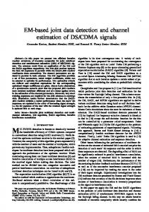
We next present numerical results for the proposed scheme using the IEEE-4 bus system (c.f. Fig. 2). Note that in this case the state status is characterized by a 3-dimensional vector, i.e., x ∈ R3 (the phase angle of bus 1 is taken as the reference). In Fig. 2, it is seen that there are eight measurements collected by meters, thus the topology is characterized by a 8-by-3 matrix, i.e., H ∈ R8×3 . Since the impedances of all links are known beforehand, we assume that they are of unit values without loss of generality. Here, instead of considering all possible forms of H , we narrow down the candidate grid topologies to the outage scenarios. In particular, as given in (70), H 0 represents the default topology matrix, and {H i , i = 1, 2, 3, 4} correspond to the scenarios where the links {l1−2 , l2−3 , l3−4 , l4−1 } (li−j denotes the link between bus i and bus j ) break down, respectively. We use the following distributions for the state vector x under the hypotheses {Hi }.

H0 : x ∼ N (π/5 × 1, π 2 /9 × I), H1 : x ∼ N (2π/5 × 1, π 2 /16 × I), H2 : x ∼ N (3π/5 × 1, π 2 /25 × I), H3 : x ∼ N (4π/5 × 1, π 2 /36 × I), H4 : x ∼ N (π × 1, π 2 /4 × I),

where ai = 0.2, bi = 0.8, ∀i, 1 is the vector of ones and I is the identity matrix. The measurements are contaminated by the white Gaussian noise wt ∼ N (0, I). The goal is to decide among the five candidate DRAFT

November 7, 2014

29

grid topologies, and meanwhile, to estimate the state vector. θ2



P1

   P1−2     P2     P2−3   H0 =   P3    P3−4     P4    P4−1 

         H2 =          

−1

θ3

−1



0

−1

0

2

−1

1

−1

−1

2

0

1

0

−1

0

0

0

−1

−1

0

0

1

0

0

0

0

0

0

1

−1

0

1

−1

0

−1

2

0

0

1

θ4



−1    0     0     0  ,   −1    −1     2    1

         ,         



         H1 =          



         H3 =          

−1

0

0

−1



  0    1 −1 0    1 −1 0  ,  −1 2 −1    0 1 −1    0 −1 2   0 0 1 0

0

0

−1

−1

0

0

2

−1

0

1

−1

0

−1

1

0

0

0

0

0

0

1

0

0

1



         ,         



         H4 =          

−1

0

0

−1

0

0

2

−1

0

1

−1

0

−1

2

−1

0

1

−1

0

−1

1

0

0

0



         .         

(70)

Since SPRT is not applicable in the multi-hypothesis case, we compare the proposed sequential joint detection and estimation (SJDE) scheme with the combination of maximum likelihood (ML) detector and MMSE estimator, equipped the stopping time given in (60). The ML detector uses the decision function   (71) dT = arg max aj pj {y t }T t=1 j

at the optimum stopping time presented in Proposition 3, hence is not a completely conventional scheme. Fig. 3 illustrates that SJDE [i.e., the hybrid ML & MMSE detector, given by (61)] significantly outperforms this combination [i.e., the conventional ML detector in (71)] in terms of the overall detection and estimation performance measured by the combined cost function, introduced in (58). We see that November 7, 2014

DRAFT

30

13

SJDE ML & Est.

12

Average stopping time

11 10 9 8 7 6 5 4 3 0.7

Fig. 3.

0.8

0.9

1

1.1

1.2

Target accuracy, α

1.3

1.4

Average stopping time vs. target accuracy level for SJDE and the combination of ML detector & MMSE estimator

equipped with the stopping rule of SJDE.

SJDE requires smaller average number of samples than ML & Est. to achieve the same target accuracy. Specifically, with small average sample size (i.e., stopping time), the improvement of SJDE is substantial. This is because smaller sample size causes larger estimation cost ∆jT , which in turn emphasizes the advantage of the proposed detector over the conventional ML detector. In fact, in smart grid monitoring, the typical sample size is small since the system state evolves quickly, and thus there is limited time to estimate the current state. VI. C ONCLUSION We have developed a general framework for optimum sequential joint detection and estimation, considering the problems in which simultaneous detection and estimation with minimal sample size is of interest. The proposed framework guarantees the best overall detection and estimation performance under a Bayesian setup while minimizing the sample size. The conventional separate treatment of the two DRAFT

November 7, 2014

31

subproblems has been shown to be strictly suboptimal since the optimum detector and estimators are strongly coupled with each other. We have also showed how the theoretical results, that are derived for a general model, apply to commonly used LQG models, including dynamic spectrum access in cognitive radio and state estimation in smart grid. We have supported the theoretical findings with numerical results. R EFERENCES [1] Y. Yılmaz, Z. Guo, and X. Wang, “Sequential Joint Spectrum Sensing and Channel Estimation for Dynamic Spectrum Access,” IEEE J. Sel. Areas Commun., to be published, Nov. 2014, available at http://arxiv.org/pdf/1401.6134v1.pdf [2] J. Chen, Y. Zhao, A. Goldsmith, and H. V. Poor, “Optimal Joint Detection and Estimation in Linear Models,” in Proc. IEEE 52nd Annual Conference on Decision and Control (CDC), pp. 4416–4421, Dec. 2013. [3] B.-N. Vo, B.-T. Vo, N.-T. Pham and D. Suter, “Joint detection and estimation of multiple objects from image observations,” IEEE Trans. Signal Process., vol. 58, no. 10, pp. 5129–5141, Oct. 2010. [4] A. Tajer, G.H. Jajamovich, X. Wang, and G.V. Moustakides, “Optimal Joint Target Detection and Parameter Estimation by MIMO Radar,” IEEE J. Sel. Topics Signal Process., vol. 4, no. 1, pp. 127–145, Feb. 2010. [5] G.H. Jajamovich, A. Tajer, and X. Wang, “Minimax-Optimal Hypothesis Testing With Estimation-Dependent Costs,” IEEE Trans. Signal Process., vol. 60, no. 12, pp. 6151–6165, Dec. 2012. [6] D. Middleton, and R. Esposito, “Simultaneous optimum detection and estimation of signals in noise”, IEEE Trans. Inf. Theory, vol. 14, no. 3, pp. 434–444, May 1968. [7] Y. Yılmaz, G.V. Moustakides, and X. Wang, “Sequential Joint Detection and Estimation,” SIAM Theory Probab. Appl., to be published, available at http://arxiv.org/pdf/1302.6058v4.pdf [8] O. Zeitouni, J. Ziv, and N. Merhav, “When is the generalized likelihood ratio test optimal?”, IEEE Trans. Inf. Theory, vol. 38, no. 5, pp. 1597–1602, Sept. 1992. [9] G.V. Moustakides, “Optimum Joint Detection and Estimation,” in Proc. IEEE International Symposium on Information Theory (ISIT), pp. 2984–2988 July 2011, [10] A. Fredriksen, D. Middleton, and D. Vandelinde,

“Simultaneous Signal Detection and Estimation Under Multiple

Hypotheses”, IEEE Trans. Inf. Theory, vol. 18, no. 5, pp. 607–614, Sept. 1972. [11] T.G. Birdsall, and J.O. Gobien, “Sufficient Statistics and Reproducing Densities in Simultaneous Sequential Detection and Estimation”, IEEE Trans. Inf. Theory, vol. 19, no. 6, pp. 760–768, Nov. 1973. [12] B. Bayg¨un, and A.O. Hero III, “Optimal Simultaneous Detection and Estimation Under a False Alarm Constraint”, IEEE Trans. Inf. Theory, vol. 41, no. 3, pp. 688–703, May 1995. [13] G.V. Moustakides, G.H. Jajamovich, A. Tajer, and X. Wang, “Joint Detection and Estimation: Optimum Tests and Applications,” IEEE Trans. Inf. Theory, vol. 58, no. 7, pp. 4215–4229, July 2012. [14] A. Wald, Sequential Analysis, Wiley, New York, NY, 1947. [15] Z. Govindarajulu, Sequential Statistics, World Scientific Publishing, Hackensack, NJ, 2004. [16] B. Efron, and D.V. Hinkley, “Assessing the accuracy of the maximum likelihood estimator: Observed versus expected Fisher information,” Biometrika, vol. 65, no. 3, pp. 457–487, 1978. [17] B.K. Ghosh, “On the attainment of the Cramer-Rao bound in the sequential case,” Seq. Anal., vol. 6, no. 3, pp. 267–288, 1987. [18] B.K. Ghosh, and P.K. Sen, Handbook of Sequential Analysis, Marcel Dekker, New York, NY, 1991. November 7, 2014

DRAFT

32

[19] P. Grambsch, “Sequential sampling based on the observed Fisher information to guarantee the accuracy of the maximum likelihood estimator,” Ann. Statist., vol. 11, no. 1, pp. 68–77, 1983. [20] G. Fellouris, “Asymptotically optimal parameter estimation under communication constraints,” Ann. Statist., vol. 40, no. 4, pp. 2239–2265, Aug. 2012 [21] Y. Yılmaz, and X. Wang, “Sequential Decentralized Parameter Estimation under Randomly Observed Fisher Information,” IEEE Trans. Inf. Theory, vol. 60, no. 2, pp. 1281–1300, Feb. 2014. [22] H.L. Van Trees, and K.L. Bell, Detection Estimation and Modulation Theory, Part I (2nd Edition), Wiley, Somerset, NJ, 2013. [23] Q. Zhao and B. M. Sadler, “A survey of dynamic spectrum access: Signal processing, networking, and regulatory policy,” IEEE Signal Processing Mag., vol.24, no. 3, pp. 79–89, May 2007. [24] Y. C. Liang, Y. Zeng, E. C. Y. Peh, and A. T. Hoang, “Sensing-throughput tradeoff for cognitive radio networks,” IEEE Trans. Wireless Commun., vol.7, no. 4, pp. 1326–1337, Apr. 2008. [25] Y. Chen, Q. Zhao, and A. Swami, “Joint design and separation principle for opportunistic spectrum access in the presence of sensing errors,” IEEE Trans. Inf. Theory, vol. 54, no. 5, pp. 2053–2071, May 2008. [26] X. Kang, Y. C. Liang, A. Nallanathan, H. K. Garg, and R. Zhang, “Optimal power allocation for fading channels in cognitive radio networks: ergodic capacity and outage capacity,” IEEE Trans. Wireless Commun., vol. 8, no.2, pp. 940–950, Feb. 2009. [27] L. Musavian and S. Aissa, “Capacity and power allocation for spectrum sharing communications in fading channels,” IEEE Trans. Wireless Commun., vol. 8, no.1, pp. 148–156, 2009. [28] X. Kang, Y. C. Liang, H. K. Garg, and L. Zhang, “Sensing-based spectrum sharing in cognitive radio networks”, IEEE Trans. Veh. Technol., vol. 58, no. 8, pp. 4649–4654, Oct. 2009. [29] Z. Chen, X. Wang, and X. Zhang, “Continuous power allocation strategies for sensing-based multiband spectrum sharing,” IEEE J. Sel. Areas Commun., vol. 31, no. 11, pp. 2409–2419, Nov. 2013. [30] Y. Li, “Pilot-symbol-aided channel estimation for OFDM in wireless systems,” IEEE Trans. Veh. Technol., vol. 49, no. 4, pp. 1207–1215, July 2000. [31] A. Sahai, R. Tandra, S. M. Mishra, and N. Hoven, “Fundamental design tradeoffs in cognitive radio systems,” in Proc. of Int. Workshop on Technology and Policy for Accessing Spectrum, Aug. 2006. [32] Y. Yılmaz, G.V. Moustakides, and X. Wang, “Cooperative sequential spectrum sensing based on level-triggered sampling,” IEEE Trans. Signal Process., vol. 60, no. 9, pp. 4509–4524, Sep. 2012. [33] Y. Huang, S. Werner, J. Huang, N. Kashyap, and V. Gupta “State Estimation in Electric Power Grids: Meeting New Challenges Presented by the Requirements of the Future Grid,” IEEE Signal Processing Mag., vol.29, no. 5, pp. 33–43, Sept. 2012. [34] Y. Huang, H. Li, K.A. Campbell, and Z. Han “Defending False Data Injection Attack On Smart Grid Network Using Adaptive CUSUM Test,” 45th Annual Conference on Information Sciences and Systems (CISS), 2011 [35] Y. Huang, M. Esmalifalak, H. Li, K.A. Campbell, and Z. Han “Adaptive Quickest Estimation Algorithm for Smart Grid Network Topology Error,” IEEE Syst. J., vol. 8, no. 2, pp. 430–440, 2014. [36] Y. Zhao, A. Goldsmith, and H. V. Poor “On PMU location selection for line outage detection in wide-area transmission networks,” IEEE Power and Energy Society General Meeting, 2012 [37] Y. Zhao, R. Sevlian, R. Rajagopal, A. Goldsmith, and H. V. Poor “Outage Detection in Power Distribution Networks with Optimally-Deployed Power Flow Sensors,” IEEE Power and Energy Society General Meeting, 2013

DRAFT

November 7, 2014