on websites during high click rates on online advertisements. (click fraud detection) or optimizing routing in peer-to-peer networks. II. IP DENSITY ESTIMATION.
Server-side Prediction of Source IP Addresses using Density Estimation Markus Goldstein∗ , Matthias Reif∗ , Armin Stahl∗ and Thomas Breuel∗† ∗ German
Research Center for Artificial Intelligence DFKI GmbH † Technical University of Kaiserslautern Research Group Image Understanding and Pattern Recognition (IUPR) D-67663 Kaiserslautern, Germany Email: {goldstein,reif,stahl,breuel}@iupr.dfki.de
Abstract—Source IP addresses are often used as a major feature for user modeling in computer networks. Particularly in the field of Distributed Denial of Service (DDoS) attack detection and mitigation traffic models make extensive use of source IP addresses for detecting anomalies. Typically the real IP address distribution is strongly undersampled due to a small amount of observations. Density estimation overcomes this shortage by taking advantage of IP neighborhood relations. In many cases simple models are implicitly used or chosen intuitively as a network based heuristic. In this paper we review and formalize existing models including a hierarchical clustering approach first. In addition, we present a modified k-means clustering algorithm for source IP density estimation as well as a statistical motivated smoothing approach using the Nadaraya-Watson kernel-weighted average. For performance evaluation we apply all methods on a 90 days real world dataset consisting of 1.3 million different source IP addresses and try to predict the users of the following next 10 days. ROC curves and an example DDoS mitigation scenario show that there is no uniformly better approach: kmeans performs best when a high detection rate is needed whereas statistical smoothing works better for low false alarm rate requirements like the DDoS mitigation scenario.
I. I NTRODUCTION User modeling is an important task for applications to understand traffic flows and user behavior at the server-side. The results of user models can be used for a variety of applications to predict future situations or classify current states with machine learning technologies. Use case scenarios include Distributed Denial of Service (DDoS) attack detection or mitigation [1][2][3][4], quality of service (QoS) [5], click fraud detection[6] and traffic forecasting in general. In peerto-peer (P2P) overlay networks, IP models can also be used for optimizing request routing [7]. Different machine learning techniques are used to train a classifier (model) with previously observed data and then usually an online decision is made by the system based on the actual traffic. In this context, also outlier detection methods are often used if only one class is known. If, for example, an Intrusion Prevention System wants to mitigate DDoS attacks, it usually has only seen the normal traffic class before and it has to detect the outlier class from the fact that it behaves differently. DDoS attacks are a major menace in the internet today. Malicious hackers build botnets through infecting a large number of PCs (bots or zombies). Then, they combine their bandwidth and computational power in order to overload a publicly available service and denial it for legal users.
There are multiple strategies with dealing with DDoS attacks, whereas practically applicable ones are near-target filtering solutions. An overview of state-of-the-art mitigation research is given by Dittrich [8] and Mirkovic et al [9]. All near-target solutions have in common, that they try to estimate normal user behavior based on IP packet header information. During an attack, outliers are detected and denied. One parameter all methods have in common, is the source IP address of the users, which seems to be a highly discriminant feature for DDoS traffic classification. However, the methods of storing IP addresses and estimating their density in the huge IP address space, are different. We give in Section III an overview, which methods are implicitly or directly chosen. Furthermore, we introduce two new statistically based methods in Sections V and VI for IP density estimation: one is based on k-means clustering and the other is a kernel density estimation approach. In Section VII we compare the different methods with a standard pattern recognition evaluation based on real network data: given a training set with previously observed IP addresses we try to predict whether an IP address will be included in an unknown test set representing future source IP addresses. Furthermore, we investigate Receiver Operating Characteristic (ROC) curves in order to compare the adaptivity of the presented methods. Although DDoS mitigation is the most important practical application for IP density estimation, we do not restrict the following work on this topic. Our generic view on IP density estimation may be valuable to other applications as well. One might think of preferring regular customers in overload situations (flash crowd events), identifying non-regular users on websites during high click rates on online advertisements (click fraud detection) or optimizing routing in peer-to-peer networks. II. IP D ENSITY E STIMATION An IP density estimation is a one dimensional density function of the random variable S over all existing N = 232 IPv4 addresses s0 = 0.0.0.0 to s232 −1 = 255.255.255.255. The density estimation is applicable on IPv6 as well, but we stick to IPv4 in the following due to a lack of IPv6 datasets. The Probability Density Function (PDF) is used in the following, which is a normalized density function f (s),
such that
Z
∞
f (s) = 1
(1)
−∞
or in the discrete IP density scenario N −1 X
P (S = si ) = 1
(2)
i=0
where P (S = si ) = pi is the probability of an IP address si to be a source IP address that will occur in the future. Since we don’t know the true underlying PDF f ∗ (s), we try to derive a good estimation f (s) for all IP addresses using a training set of observed IP addresses. Later, in Section VII, we use a test set of IP addresses not used during training and calculate the deviation from the predicted estimation to compare the different methods. III. R ELATED W ORK In this section we review existing IP density estimation approaches. Furthermore, we formulate the often implicitly used ideas in a probabilistic way using the PDF. A. History-based IP Filtering Peng et al. [4] first proposed an algorithm called Historybased IP Filtering (HIF), a source IP density estimation for mitigating DDoS attacks. Therefore, an IP address database (IAD) contains all frequently previously seen IP addresses. During an attack, only IP addresses from the IAD are permitted and all others are blocked. The groundwork for this algorithm was introduced by Jung et al. [10] analyzing IP addresses from Code Red worm attacks. He found that source IP addresses from attack traffic have not been seen before and have a different distribution than the normal user traffic. According to Peng et al., IP addresses are added to the IAD if a certain threshold (e.g. a certain number of packets) is exceeded. Later during an attack, the decision whether an IP has to be blocked or not is binary. This means, the density estimation results in a simple step function with only two values: Zero or a positive value, which is the same for all IP addresses. The PDF can be calculated as follows: min(ns , 1) (3) f (s) = PN −1 i=0 min(nsi , 1) where ns is the number of occurrences of an IP address s in 1 the training set. This means, the probability pi is either M if there are M different IP addresses in the training set or zero if si has not been observed. The advantage of HIF is that it is efficiently computable online, also during DDoS attacks. This comes at the price, that it cannot be differentiated between users which revisit the server more often than others and is therefore a less precise density estimator. B. Adaptive History-based IP Filtering Goldstein et al. [1] presented Adaptive History-based IP Filtering (AHIF) to compensate the shortcomings of HIF: instead of using the binary decision ”seen or not seen“, histograms are used for density estimation: ns f (s) = PN −1 (4) i=0 nsi
where s does not necessarily represent a single IP address, it rather stands for a range of IP addresses (a bin of the histogram). So far, constant width networks with fixed network masks ranging from 16 up to 24 bit are used as source bins. The actual prediction Cα of the appearance of an IP address (or an IP range) is done using a threshold α over f (s): � appears f (s) > α Cα (s) = (5) does not appear otherwise During attack mitigation, the most appropriate network mask is chosen such that a maximum numbers of firewall rules is not exceeded and the attack traffic is reduced to be below the maximum server capacity. It is shown, that the adaptive method performs better in terms of predicting user IP addresses during an attack. However, neighbor relations (between source networks) are not taken into account. Kim et al. [2] use a similar approach with fixed bin sizes of only 16bit prefixes for online packet classification. Compared to AHIF using smaller bin sizes this method is less accurate, but uses less resources. C. Clustering of Source Address Prefixes Pack et al. [3] introduced algorithms for mitigating DDoS attacks by filtering source address prefixes. Unlike AHIF, network masks may be at different sizes. For finding the appropriate networks, the authors are using a hierarchical agglomerative clustering algorithm with single linkage. The used distance measure is defined with respect to network boundaries, which we will describe later in Section IV-A. In general, the proposed method takes both into account – the amount of requests from a source network as well as neighboring density estimation as a result of using a (generalizing) clustering method. Unfortunately, hierarchical clustering methods consume a lot of memory and it was found [1], that the presented method is not applicable in practice on large source IP datasets. IV. IP D ISTANCE M EASURES FOR IP V 4 A DDRESSES All density estimation approaches require the definition of an appropriate distance measure between two IP addresses si and sj . In the AHIF approach the bin size of the histogram defines the distance: if two IP addresses have the same prefix based on the used network mask, the distance is zero. If they do not fall into the same bin, the distance is infinity. The most common way of a distance measure is to use the Euclidean distance, which is in the one dimensional IP domain simply the absolut value of the difference between two 32bit integer values: ∆Eucl (si , sj ) = |si − sj |
(6)
A. Xor The IPv4 address space is partitioned into multiple variable length subnets, which are individually assigned and routed to customers. Therefore one can assume that IP addresses in the same subnet are more similar to each other than two IP addresses in different networks. For example, if a department runs the network 131.246.10.0/24, the IP addresses 131.246.10.1 and 131.246.10.3 are naturally more similar than
800
M source IP addresses. The k-means algorithm [11] seems to be more appropriate for the density estimation scenario, which cuts down the memory requirement to O(M · K), where K is the number of cluster centers. Also, the quadratic runtime of hierarchical algorithms is reduced to linear complexity. K-means was also used in a similar scenario by Agrawal et al. [7] for identifying nearby host clusters in peerto-peer overlay networks. Instead of estimating densities from cluster centers, they are used to optimize P2P request routing. Algorithm 1 shows the pseudo-code of the used k-means algorithm.
∆Eucl ∆Xor ∆Xor+ 700
Calculated Xor/Xor+ Distance
600
500
400
300
200
100
0 -200
Fig. 1.
-100
0 Euclidean Distance
100
200
Different distance measures for the IP address 131.246.10.180
the IP addresses 131.246.9.255 and 131.246.10.1 although their Euclidean distance is smaller. Taking this fact into account during IP density estimation, we used the distance measure proposed by Pack et al. [3]: Xor the two IP addresses in integer notation together and keep the highest order bit set and set all lower bits to 0. This results in a maximum of 32 different distances ranging from 20 to 231 . For example, the distance of 346 and 365 is 32:
Algorithm 1 The k-means algorithm 1: Input 2: S = s1 , . . . , si : training data source IP addresses 3: k: initial number of clusters 4: ∆(si , sj ): Distance function for IPs si ,sj 5: 6: 7: 8: 9: 10: 11: 12: 13: 14:
Output C = c1 , . . . , ck : cluster centroids B = b1 , . . . , bk : number of IPs belonging to ck function K - MEANS(S, k, ∆()) C ←random set of S while m has changed or iter < maxiter do for all si ∈ S do m(si ) ← arg min(dist(si , cj )) j∈{1...k}
346 365 32
101011010 101101101 000100000
15: 16:
To be more formal, the distance can be calculated using Equation 7: blog2 (si ⊕sj )c
∆Xor (si , sj ) = 2
(7)
B. Xor+ A possible downside of using the Xor distance measure might be the fact that distances within a specific network mask are always constant, regardless of variation within this subnet. For example, the IP addresses 131.246.9.0 and 131.246.10.0 have the same distance (29 = 512) as the addresses 131.246.9.0 and 131.246.10.255. To get a smoother distance measure, the Xor+ distance is introduced: First the Xor distance is calculated and then the Euclidean distance is added: ∆Xor+ (si , sj ) = 2blog2 (si ⊕sj )c + |si − sj |
(8)
This results in a linear increase between two network based distance jumps as illustrated in Figure 1. Referring to the example above, the first distance is 768 and the second is 1023. V. U SING K - MEANS FOR IP D ENSITY E STIMATION In order to perform clustering of IP addresses in practice on large real world data sets, the memory consumption has to be reduced. Using hierarchical clustering methods yield to store distance matrices in memory, which are usually O(M 2 ) having
17: 18: 19: 20: 21:
for all cj ∈ C do cj ← average(∀sj with m(sj ) = cj ) Remove duplicates from C iter ← iter + 1 for all si ∈ S do bm(si ) ← bm(si ) + 1 return C, B
Since source IP addresses usually show up more than one time, a caching technique was used in order to speed up the distance and the centroid calculation (not shown in Algorithm 1). For the distance measure ∆, the Xor distance measure from Section IV-A or the Euclidean distance can be used. Using a non-Euclidean distance measure like Xor, one has to take care of the average function, which is in fact a problem using Xor+. Since k-means is an expectationmaximization (EM) algorithm, the average must be calculated with respect to the distance function. Otherwise, the expectation and maximization steps may have no common target value and the algorithm may oscillate. Luckily the arithmetic mean (based on the Euclidean distance) is the same as the mean based on the Xor distance measure. Since this fact has not yet been formally proven, we assume that it is at least a sufficient estimation. Once the cluster centers are calculated, a variable surrounding area has to be defined. Within this surrounding area the model predicts to see the IP address again in the test set. Outside of the area (far away from the cluster centers), the model assumes no source IP addresses. Pack et al. [3] suggests to define the area by reducing the prefix length. This method
bj wj = Pk
i=1 bi
(9)
This weighting yields to larger surrounding areas in highdensity clusters and smaller areas in less dense clusters. This easy heuristic yields to better density estimation although it is not proven to be statistically optimal. VI. S UBNET B OUNDARY S ENSITIVE S MOOTHING Applying the idea of using kernel density estimation for IP density estimation we introduce Subnet Boundary Sensitive Smoothing (SBSS). First, a normalized histogram count of IP addresses is created like in AHIF. Then, the histogram is smoothed using a kernel density estimator [12]. Again, the structure of the IP address space can be taken into account by using the Xor or Xor+ distance measure. The first estimation of the probability density function f (s) over the address space is based on the number of occurrences ns0 , . . . , nsN −1 of every single IP address s and equivalent to AHIF (see Section III-B): ns (10) f (s) = PN −1 i=0 nsi and pi = f (si ) is the probability that the next occurring IP address is si . Now we assume that if an IP address s is likely to occur next, IP addresses in a defined neighborhood close to s can also occur next with a quite high probability, which is due to the undersampling of the large IP address space. Therefore the probability of all IP addresses si in the neighborhood around s are increased dependently from the probability ps and the distance ∆(s, si ). Every probability ps of each single IP address influences the new probabilities of the IP addresses in its neighborhood and vice versa. The Nadaraya-Watson kernel-weighted average [12] with a kernel Kλ is used for smoothing: PN −1 Kλ (s, si )pi (11) pˆs = Pi=0 N −1 i=0 Kλ (s, si ) The new probability pˆs of s is the weighted and normalized sum of all probabilities of every IP address si . The actual values for the weights are defined by the kernel Kλ . A. The Kernel The kernel Kλ is basically a function over the distance ∆(s, si ) of two data points s and si and uses a predefined window size λ of the distance: � � ∆(s, si ) Kλ (s, si ) = D (12) λ
The actual kernel function D can be different and depends on the true underlying unknown distribution. Typical kernels are the Epanechnikov quadratic kernel, the Tri-cube and the Gaussian kernel: � 3 2 4 (1 − t ) |t| ≤ 1 Epanechnikov: D(t) = (13) 0 otherwise � (1 − |t|3 )3 |t| ≤ 1 Tri-Cube: D(t) = (14) 0 otherwise 1 2 1 Gaussian: D(t) = √ e− 2 t (15) λ 2π For Gaussian kernels the window size λ is equivalent to the standard deviation σ of the Gauss function. All three kernels count observations closer to the target point s with higher weights: the higher the distance of the second data point si to s, the smaller its influence. Experiments with the different kernels have shown that the kernel function itself plays a minor role in terms of classification performance (see Section VII-D). As a distance measure ∆(s, si ) of two IP addresses the Xor and the Xor+ measures as well as the Euclidean distance are used (see Section IV). In Figure 2 it is observable that the Euclidean distance measure generates a more continuous density estimation function in contrast to the distance measures based on the Xor operation that reflect the subnet structure of the IP address space in a better way. unsmoothed Distance Measure ∆Xor Distance Measure ∆Xor+ Distance Measure ∆Eucl
P(s)
again adopts the area to the natural IP network partitions like the Xor distance measure. Besides this area growing algorithm we suggest a second heuristic method. Since centroids might contain a different number of training data points, they can be differently important. Our modification of the area growing algorithm takes this into account and grows the areas around the centroids with a weighting factor wj which represents the amount of data points of the specific centroid directly calculated from B in Algorithm 1:
IP address
Fig. 2. Different distance measures using a Gaussian kernel with window size λ = 4
Finally, the window size λ controls how large the neighborhood (which influences pˆs ) is. If it is very small, only IP addresses si closed by influence pˆs and the overall smoothing effect is not striking. When using a window size that is too big, this may lead to an oversmoothed result and may not represent the given data proper. In general it is a challenge to find the correct kernel window size. Turlach [13] shows different methods, whereas we evaluated multiple sizes. If the window size λ is close to 0 meaning that no IP address influences another and therefore no actual smoothing is performed, this method is equivalent to the AHIF approach discussed in Section III-B.
B. Prediction In order to evaluate this approach we finally have to predict if an IP address appears in the test set or not. This decision is done similar to the AHIF method by using a threshold α over the smoothed probability density function from Equation (11): � appears pˆs > α Cα (s) = (16) does not appear otherwise The actual evaluation of this approach including the discussion of the influence of the parameter α can be found in Section VII-D C. Pseudo Code Unoptimized pseudo code of the SBSS approach is listed in Algorithm 2. A lot of runtime improvements can be achieved by a proper implementation, which first checks in which IP ranges smoothing makes sense at all before actually performing it. However, it is obvious that the runtime increases with a growing window size λ since more neighboring points have to be taken into account. Algorithm 2 The SBSS algorithm 1: Input 2: ∆(a, b): Distance function for IP addresses a, b 3: Kλ : Kernel 4: λ: Window size 5: N = n0 , . . . , n232 −1 : No. of occurrences of IPs 6: 7: 8: 9: 10: 11: 12: 13: 14: 15: 16: 17: 18: 19: 20: 21: 22: 23: 24: 25: 26: 27: 28: 29:
Output C = c0 , . . . , c232 −1 : Predictions of IP addresses function SBSS(α) σ←0 for all IP addresses s σ ← σ + ns for all IP addresses s ps ← ns /σ for all IP addresses s pˆs ← Smooth(s) if pˆs > α then cs ← appears else cs ← does not return C
do do do
appear
function S MOOTH(s) pˆ ← 0; v ← 0 for all IP addresses si around s do calculate Kλ (s, si ) with ∆(s, si ) pˆ ← pˆ + Kλ (s, si ) · psi v ← v + Kλ (s, si ) 30: return pˆ/v
VII. E VALUATION A. Dataset Logged IP addresses of users are very sensitive data since they allow inference of user behavior or even user identi-
fication. Therefore all public available data sets anonymize IP addresses such that the original one is not disclosed. All methods securely anonymizing IP addresses have to destruct neighborhood relations [14], which makes it impossible to evaluate the proposed approaches in this paper with a public dataset. The evaluation presented in the following relies on a Apache log file obtained by the webserver www.xvid.org. It contains 53,828,308 requests from 1,284,213 different IP addresses from 200 countries over 100 days. The complete dataset was divided into 90 days of training data for creating the IP density estimator and 10 days of test data to evaluate the performance of the model. In particular, the training set contains of 48,634,123 requests from 1,168,293 different sources and the test set contains 5,194,185 requests from 135,265 IP addresses. The 90-10 division of the data set may not be representative for all application scenarios (e.g. DDoS attacks do usually not last 10 days), but for having a statistical significant evaluation, this partitioning is required. If a shorter evaluation period is used, collateral damage is usually much lower. This is due to the fact that test data close to the training data is better predictable than trends in the future. Based on the test set, receiver operating characteristic (ROC) curves are computed and plotted. The detection rate (true positive rate) and the false alarm rate (false positive rate) are defined as follows: true positive true positive + false negative false positive false alarm rate = false positive + true negative detection rate =
In this context, true positive are source addresses which were predicted by the model to appear and are part of the test set whereas true negative are predicted not to appear and also actually don’t appear. If an IP address is predicted to appear but it actually doesn’t this is counted as a false positive. A false negative is an IP occurring in the test set but was predicted to be absent. From the ROC curves it can be directly derived whether a density estimator is uniformly better than another. For more quantitative comparison, the area under curve (AUC) is also computed. It is possible that a ROC curve is incomplete because the function is not defined for every value pair of false alarm rate and detection rate. At the bottom left point (0, 0) the method predicts no IP address to occur resulting in a perfect false alarm rate with the worst possible detection. By changing the parameter of the used method (e.g. decreasing the threshold α for SBSS) more IP addresses are classified to appear, but causing also a higher false alarm rate. If the parameter is set to its limit (e.g. α = 0 in SBSS), no more IP addresses can be predicted to appear causing the ROC to end at this point. A possible procedure for completing the missing part of the curve to the point (1,1) is to iteratively select more and more IP addresses randomly an predict them to appear. This procedure leads to a straight line continuing the curve. This is useful for (1) determining if an approach is uniformly better than another and (2) to compute the AUC for this method. In
the following we will omit plotting this interpolation for the sake of visualization clarity.
1
B. Evaluation of HIF and AHIF For evaluating the AHIF approach ROC curves for different network sizes were created by varying the decision threshold α of Equation (5). Since the simpler HIF method does not use a variable threshold, the result of its evaluation is not a ROC curve but a single point. It is equivalent to the top right point of the according ROC curve of the AHIF approach. This illustrates that the AHIF approach achieves at least the performance of HIF but provides more flexibility since HIF is limited to one pair of values of detection rate and false alarm rate.
0.8
Efficiency
0.6
0.4
0.2 k-means (100 centroids) k-means (1000 centroids) k-means (5000 centroids) k-means (10000 centroids) k-means (20000 centroids) 0 0
0.2
1
0.4 0.6 Collateral Damage
0.8
1
(a) Standard area growing 1
0.8
0.6 Efficiency
Detection Rate
0.8 0.6
0.4
0.4 0.2
HIF (16bit prefix) HIF (24bit prefix) HIF (32bit prefix) AHIF (16bit prefix) AHIF (24bit prefix) AHIF (32bit prefix)
0.2 k-means (100 centroids) k-means (1000 centroids) k-means (5000 centroids) k-means (10000 centroids) k-means (20000 centroids)
0 0
0.2
0.4
0.6
0.8
1
False Alarm Rate
Fig. 3. Using smaller network prefixes for HIF and AHIF increases the detection rate with the downside of having a higher false alarm rate
0 0
0.2
0.4 0.6 Collateral Damage
0.8
1
(b) Weighted area growing Fig. 4. Running k-means with different initial number of centroids based on the Xor distance measure. 1
0.8
0.6 Efficiency
C. Evaluation of K-Means 1) Different Area Growing Algorithms: In Section V two growing algorithms for the surrounding area were introduced: (1) constantly shrinking the network bitmask of the centroid and (2) taking a weight factor into account that represents the number of IP addresses belonging to a cluster centroid based on the first method. Varying these parameters a ROC can be calculated. Figure 4(a) illustrates the results using (1) and 4(b) using (2). Using a different number k ∈ [100, 1000, 5000, 10000, 20000] of initial centroids result in different performance. Using more centroids obviously leads to better results, but coming at the price of longer runtimes. The k-means algorithm either runs until no changes of cluster belongings were detected or maxiter = 40 was reached as listed in Algorithm 1. 2) Distance Measure ∆: The results based on the Xor distance measure can be obtained from Figure 4. Furthermore, Figure 5 gives a direct comparison of both distance measures based on the weighted area growing method for 100 and 20,000 initial centroids. Surprisingly, the Xor distance measure performs not as good as the Euclidean version. A possible explanation for this observation might be the fact, that distances calculated with the Xor method can be quite large – leading to few changes in data points belonging to a centroid.
0.4
0.2 k-means (20000 centroids, Distance Measure ∆Xor) k-means (20000 centroids, Distance Measure ∆Eucl) k-means (100 centroids, Distance Measure ∆Xor) k-means (100 centroids, Distance Measure ∆Eucl)
0 0
0.2
0.4 0.6 Collateral Damage
0.8
1
Fig. 5. K-means performs generally better when using the distance measure ∆Eucl (here using the weighted area growing algorithm).
3) Stability: One possible drawback of using k-means is the random initialization of the initial centroids. Within the expectation maximization loop unfortunate initial chosen
1
0.8
Detection Rate
centroids may cause the algorithm to stuck into a local minima and thus not returning the optimal result. In order to test this effect on the results of density estimation, we performed 10 experiments running the most error prone setup with 100 initial centroids and the Xor distance measure. The results with the weighted area growing algorithm are illustrated in Figure 6 and show that the approach is quite stable.
0.6
1
0.4
0.8
0.2
0.6
0
SBSS (Window Size λ=1) SBSS (Window Size λ=128) Efficiency
0
0.2
0.4
0.6
0.8
1
False Alarm Rate
Fig. 7. A larger window size in SBSS can increase the detection rate dramatically with just a minor increase of false alarm rate (here using a Gaussian kernel and the Xor distance measure).
0.4
0.2
1
k-means min/max deviation 0 0.2
0.4 0.6 Collateral Damage
0.8
0.8
1
Fig. 6. Small min/max deviations show the stability of the k-means method (here using 100 centroids, the Xor distance measure and the weighted area growing).
D. Evaluation of SBSS SBSS was also evaluated with multiple distance measures (Xor, Xor+, Euclidean), different kernel types (Epanechnikov, Tri-Cube, Gaussian) and window sizes. The shown ROC curves were computed by varying the classification threshold α of Equation (16). 1) Effect of the Window Size λ: As described earlier the window size affects the quality of the smoothing algorithm. As illustrated in Figure 7, a larger window size causes higher detection rate with a small increase of false alarms compared to the procedure of randomly selecting IP addresses. But in contrast increasing the window size too much leads to worse performance in total. 2) Influence of Kernel Type Kλ : Another parameter of the SBSS algorithm is the kernel type used for the weighted average. Figure 8 shows that all three kernel types obtain almost the same ROC at balanced window sizes. 3) Distance Measure ∆: Three distance measures were evaluated: the Xor and Xor+ distance measure as well as the Euclidean distance (see Section IV). Similar to the kernel type, this parameter has only minor influence to the prediction performance. E. Performance Comparison of (A)HIF, SBSS and K-means In Figure 9 the comparison of all presented methods is illustrated. Since HIF produces only a single point in the ROC plot, this method cannot be directly compared. For all other methods, the best parameter setting was chosen each. In particular, AHIF used a 20bit network prefix mask, SBSS was calculated using a Gaussian kernel with Euclidean distance and a window size of 128. K-means was computed using
Detection Rate
0
0.6
0.4
0.2 SBSS (Kernel Kλ=Gaussian, Window Size λ=16) SBSS (Kernel Kλ=Epanechnikov, Window Size λ=1024) SBSS (Kernel Kλ=Tri-Cube, Window Size λ=1024) 0 0
0.2
0.4
0.6
0.8
1
False Alarm Rate
Fig. 8. Different kernel types for SBSS achieve almost equal performance at balanced window sizes (here using the Xor distance measure).
20,000 initial centroids, the weighted area growing and also the Euclidean distance. It can be obtained, that SBSS works slightly better than the not smoothed AHIF and k-means performs worse than AHIF and SBSS. However, in the area where SBSS and AHIF are not defined and estimated by a staight line, k-means performs better (detection rate > 0.97). If a small false alarm rate is required, (< 0.24), SBSS should be preferred. Table I compares the overall performace (AUC) of the presented approaches. It can be seen, that SBSS performs in general better than k-means. F. DDoS Performance Comparison DDoS flooding attacks using forged source IP addresses such as SYN attacks, ICMP or UDP packet floods cannot be blocked with simple firewall rules in many cases. If a DDoS attack is targeting a name server with forged DNS requests, it is not possible to filter requests with port or protocol parameters. Instead, an IP density estimation model can be used to filter malicious requests. In this context, the terms efficiency (correctly blocking illegal sources)
TABLE I C OMPARING AUC VALUES OF AHIF, SBSS AND K - MEANS WITH OPTIMAL PARAMETER SETTINGS
Method AHIF (20bit prefix) SBSS (Kλ =Gaussian, ∆Eucl , λ = 128) k-means (20000 centroids, ∆Eucl , weighted)
AUC 0.962 0.970 0.954
and collateral damage (denying legal users) are used to evaluate the quality of a DDoS mitigation system. Since this is the complementary event of (legal) IP density estimation we can define efficiency = 1 - false alarm rate and collateral damage = 1 - detection rate Goldstein et al. [1] suggests to run the server right below its maximum capacity in order to minimize collateral damage and mitigate the attack. In Table II we compare typical effectivity target rates of 90%, 95% and 99% and compare the results. We do not consider the IP address density estimation as a full DDoS mitigation method, it rather is a better estimation of one feature. For example, it could be easily plugged into the PacketScore framework by Kim et al [2]. TABLE II VALUES OF COLLATERAL DAMAGE IN PERCENT FOR CERTAIN REQUIRED EFFICIENCIES (90%, 95% AND 99%) AS EXAMPLES FOR DD O S SCENARIOS
AHIF • 32bit prefixes • 20bit prefixes • 16bit prefixes SBSS • window size λ = 4 • window size λ = 32 • window size λ = 128 k-means • 100 centroids • 5000 centroids • 20000 centroids
90.0
95.0
99.0
77.15 4.13 9.43
81.44 18.71 28.25
85.87 65.04 71.17
23.51 4.53 3.58
24.81 14.88 14.88
61.68 61.81 61.52
33.75 16.45 12.29
60.45 37.34 30.17
91.40 80.52 77.07
1
Detection Rate
0.8
0.6
0.4
0.2 HIF (20bit prefix) AHIF (20bit prefix) SBSS (Kernel Kλ=Gaussian, Distance Measure ∆Xor, Window Size λ=128) K-Means (20000 centroids, Distance Measure ∆Eucl, Weighted Area Growing)
0 0
0.2
0.4
0.6
0.8
1
False Alarm Rate
Fig. 9.
Comparison of the ROC curves of HIF, AHIF, k-means and SBSS
VIII. C ONCLUSION As shown in the previous Section, there is no uniformly better approach. Depending on the application and desired target variable, either SBSS or k-means clustering is the right choice in terms of performance. In the example DDoS mitigation scenario with forged source IP addresses one might prefer SBSS as the method of choice. However, computational complexity might also be an important factor as well. If, for example, the model must be computed in almost real time, AHIF should be preferred. Smoothing is a very compute intense task and one has to decide if the small benefit of SBSS is worth the computation time. For example, if running on router hardware in a time critical environment, AHIF might be the first choice. On the other hand, if precision is more important than computation time and the detection rate must be high (like one would expect in the click fraud detection scenario), k-means might be the better choice. In general it was found, that a specific distance measure taking internet subnet partitioning into account does not improve results significantly. Using k-means as density estimator, it was even contra productive. Xor in particular seems to have the drawback of generating too large and therefore insuperable distances. R EFERENCES [1] M. Goldstein, C. Lampert, M. Reif, A. Stahl, and T. Breuel, “Bayes optimal ddos mitigation by adaptive history-based ip filtering.” Los Alamitos, CA, USA: IEEE Computer Society, 2008, pp. 174–179. [2] Y. Kim, W. C. Lau, M. C. Chuah, and H. J. Chao, “Packetscore: A statistics-based packet filtering scheme against distributed denial-ofservice attacks,” IEEE Transactions on Dependable and Secure Computing, vol. 03, no. 2, pp. 141–155, 2006. [3] G. Pack, J. Yoon, E. Collins, and C. Estan, “On Filtering of DDoS Attacks Based on Source Address Prefixes,” in Proceedings of the 2nd International Conference on Security and Privacy in Communication Networks (SecureComm 2006). IEEE, 2006. [4] T. Peng, C. Leckie, and K. Ramamohanarao, “Protection from Distributed Denial of Service attack using history-based IP filtering,” in Proceedings of the IEEE International Conference on Communications (ICC 2003). Anchorage, AL, USA: IEEE, 2003. [5] Y. Yang and C.-H. Lung, “Traffic forecast in qos routing.” in Proceedings of 22nd Biennial Symposium on Communications, 2004. [6] C. Q. T. G. Inc, “How fictitious clicks occur in third-party click fraud audit reports,” 2006, available at: http://www.google.com/adwords/ReportonThirdPartyClickFraudAuditing.pdf. [7] A. Agrawal and H. Casanova, “Clustering hosts in p2p and global computing platforms,” in Proceedings of 3rd IEEE/ACM International Symposium on Cluster Computing and the Grid (CCGrid 2003), 2003. [8] D. Dittrich, “Distributed Denial of Service (DDoS) Attacks/tools,” available at: http://staff.washington.edu/dittrich/misc/ddos/. [9] J. Mirkovic, S. Dietrich, D. Dittrich, and P. Reiher, Internet Denial of Service: Attack and Defense Mechanisms (Radia Perlman Computer Networking and Security). Upper Saddle River, NJ, USA: Prentice Hall PTR, 2004. [10] J. Jung, B. Krishnamurthy, and M. Rabinovich, “Flash crowds and denial of service attacks: Characterization and implications for cdns and web sites,” in Proceedings of the International World Wide Web Conference. IEEE, 2002, pp. 252–262. [11] J. A. Hartigan and M. A. Wong, “A k-means clustering algorithm,” Applied Statistics, vol. 28, pp. 100–108, 1979. [12] T. Hastie, R. Tibshirani, and J. H. Friedman, The Elements of Statistical Learning. Springer, August 2001. [13] B. Turlach, “Bandwidth selection in kernel density estimation: A review,” 1993. [Online]. Available: http://citeseer.ist.psu.edu/214125.html [14] S. Coull, C. Wright, F. Monrose, M. Collins, and M. Reiter, “Playing devil’s advocate: Inferring sensitive information from anonymized network traces,” in Proceedings of the 14th Annual Network and Distributed System Security Symposium, 2007.