AbstractâThe radio link level delay statistics in a wireless network using adaptive modulation and coding (AMC), weighted round-robin (WRR) scheduling, and ...
Service Differentiation in Multi-Rate Wireless Networks with Weighted Round-Robin Scheduling and ARQ-Based Error Control Long B. Le, Student Member, IEEE, Ekram Hossain, Member, IEEE, and Attahiru S. Alfa, Member, IEEE
Abstract— The radio link level delay statistics in a wireless network using adaptive modulation and coding (AMC), weighted round-robin (WRR) scheduling, and automatic repeat request (ARQ)-based error control is analyzed in this paper. WRR scheduling can be used for service differentiation similar to that achievable by using the generalized processor sharing (GPS) scheduling discipline. The analytical framework presented in this paper captures physical and radio link level aspects of a multi-rate multi-user wireless network (e.g., general fading model, AMC, scheduling, error control) in a unified way. It can be used for admission control and cross-layer design under statistical delay constraints. The analytical results are validated by simulations. Typical numerical results are presented and their useful implications on the system performance are discussed. Index Terms— Adaptive modulation and coding (AMC), finite state Markov channel (FSMC), automatic repeat request (ARQ) protocol, weighted round-robin scheduling, service differentiation.
I. I NTRODUCTION Integration of data communications services into wireless networks has received increasing interests from the research community in recent years. An efficient analytical tool for performance investigation at the link layer plays a key role in engineering the wireless system and predicting the higher layer protocol performance (e.g., the transmission control protocol (TCP) performance). Analysis for link layer automatic repeat request (ARQ) protocols was done extensively in the past ( [1]- [2] and references therein). Most of the previous works in the literature, however, assumed either independent or twostate Markov channel, which allows only a single packet to be transmitted over the channel in one time slot. In fact, most (if not all) 2.5/3G wireless networks employ multirate transmission by using adaptive modulation and coding (AMC) [3], [4]. Furthermore, the existing analysis for ARQ protocols is mainly for a single-user scenario. Developing a cross-layer (physical and radio link) analytical framework for multi-rate transmission in a multi-user environment is still an open and interesting research problem. Manuscript received February 23, 2005; May 10, 2005, and July 22, 2005; accepted July 26, 2005. The editor coordinating the review of this paper and approving for publication is Romano Fantacci. This work was supported by a grant awarded to E. Hossain from the Natural Sciences and Engineering Research Council (NSERC) of Canada. This paper was presented in part at the IEEE Vehicular Technology Conference (VTC’05 Fall), Dallas, Texas, USA, September, 2005. The authors are with the Department of Electrical and Computer Engineering of University of Manitoba, Winnipeg, MB, Canada R3T 5V6, (e-mail: {long, ekram, alfa}@ee.umanitoba.ca).
Implementation of differentiated services with guaranteed quality of service (QoS) in wireless networks has been another research focus recently. The generalized processor sharing (GPS) scheduling discipline [7] (also known as the weighted fair queueing) has been widely studied as an efficient way to implement differentiated services in a multi-user environment. It can guarantee the throughput share proportional to the assigned weight of each user. Unfortunately, the exact delay statistics for this scheduling cannot be found and only deterministic or statistical delay bounds can be derived [7], [8]. These delay bounds may not be very tight, which may lead to low resource utilization. It was shown in [7] that compared with the GPS scheme, the weighted round-robin (WRR) scheduling is simpler to implement, however, the performances of these two scheduling schemes are very close to each other. In this paper, we present a cross-layer (physical and radio link) analytical framework for radio link level performance evaluation. In the physical layer, AMC is employed where the number of transmitted packets in one time slot varies depending on the channel condition. The channel is modeled by a finite state Markov channel (FSMC) model [5], [6]. An ARQ protocol is employed in the link layer to counteract the residual error of an error correction code in the physical layer. The exact queue length and delay distributions are then derived analytically. To show the usefulness of the presented model, admission control for delay-constrained applications and cross-layer design examples are illustrated. The rest of this paper is organized as follows. System model and assumptions are described in Section II. In Section III, the queueing problem is formulated and solved to obtain the desired performance metrics. The numerical and the simulation results are presented in Section IV. Conclusions are stated in Section V. II. S YSTEM M ODEL AND A SSUMPTIONS Suppose that there are µ separate radio link level queues at the base station (BS) which correspond to µ different mobile users. One common channel for downlink transmission is shared by all users in a time-division multiplexing (TDM) fashion. The transmission time is slotted and a WRR scheduler is used to schedule transmissions corresponding to the different mobiles. For the sake of simplicity, we assume that there are only two classes of users: high priority (class one) and low priority (class two). High priority users and low priority users
IEEE TRANSACTIONS ON COMMUNICATIONS, VOL. 54, NO. 2, FEBRUARY 2006
receive two and one service slots in one cycle, respectively. One cycle is defined to be the smallest interval with time slot assignments for all µ users and it repeats periodically. The receiver decodes the received packets and sends negative acknowledgments (NACKs) to the transmitter asking for retransmission of the erroneous packets (if any). In this paper, an error-free and instantaneous feedback channel is assumed so that the transmitter knows exactly if there is any transmission error at the end of each service time slot. This assumption holds in many cases because the propagation delay and the processing time for the error detection code can be very small in comparison with the time slot interval. In fact, the effect of feedback errors can be easily included in the channel model as in [1]. The delay obtained in this paper, therefore, can be regarded as the lower bound of the delay obtained with these effects. AMC is employed in the physical layer with K transmission modes corresponding to different channel states. We assume that, when the channel is in state k, the transmitter transmits ck packets. We further assume that c0 = 0 (i.e., the transmitter does not transmit in channel state 0 to avoid the high probability of transmission errors) and cK = N . The channel state information (CSI) is fed back to the transmitter to choose the suitable transmission mode. The feedback channel, therefore, carries both CSI for AMC and ACK/NACK for the ARQ protocol. To capture the variations of the multi-state Nakagami fading channel, we employ the FSMC model [6]. The received signal to noise ratio (SNR) X is partitioned into K + 1 intervals, each of which corresponds to a particular channel state. Each channel state corresponds to a unique transmission mode of AMC in the physical layer. The average packet error rate for mode k (PERk ) can be calculated as in [4]. Let Ti,j (0 ≤ i, j ≤ K) denote the transition probability from state i to state j of the channel transition matrix T, which has order (K + 1) × (K + 1). If the thresholds of the received SNR are determined, Ti,j can be calculated as in [4], where transitions are only allowed among the neighboring states [4]- [6]. Specifically, the channel transition matrix T has the following form:
2
T0,0 6 T1,0 6 6 T=6 6 0 4 0 0
T0,1 T1,1 .. . ··· ···
··· T1,2 .. .
··· ... .. .
TK −1,K −2 ···
TK −1,K −1 TK ,K −1
2
A0,3 6 A 1,4 6 6 A 6 2,5 6 6 A3,6 6 6 A7 6 P = 6 6 6 6 6 6 6 6 6 4
A0,2 A1,3 A2,4 A3,5 A6 A7
0 0
A0,1 A1,2 A2,3 A3,4 A5 A6 A7
0 TK −1,K TK ,K
A0,0 A1,1 A2,2 A3,3 A4 A5 A6 A7
3 7 7 7 7 . (1) 7 5
2
III. F ORMULATION OF THE Q UEUEING M ODEL A. Queueing Model and Analysis The queueing analysis for a target queue can be performed by using a vacation queueing model. While a particular target user is served in his assigned slots, the queue is assumed to be in service; otherwise, it is said to be in vacation. Since the queueing performances for mobile users of each class are statistically the same, we focus on one user from each class only. In the following, we analyze the queueing performance for each user class separately. For convenience, let the service period start from slot one of each cycle for each user class. Assuming that there are µ1 high priority users and µ2 = µ−µ1 low priority users, one cycle consists of L = 2µ1 + µ2 time slots. The queueing problem for both classes of users can be modeled in discrete time with one time interval equal to one time slot. Packet arrival is described by a batch Markovian arrival process (BMAP), which is represented by M + 1 substochastic matrices Um (m = 0, 1, 2, · · · , M ) each of which has order M1 × M1 [9]. The elements Um (i , j ) represent the transition from phase i to phase j with m arriving packets. With this traffic modeling, there are at most M arriving packets in one time slot and the correlation in the traffic arrival process is captured by the M1 arrival phases. The buffer is assumed to be finite with size of Q packets. We assume that packets arriving during time interval n − 1 cannot be served until time interval n at the earliest. Furthermore, packet transmissions in a time slot are assumed to finish before arriving packets enter the queue. Any arriving packet which sees the full buffer will be lost. The discrete-time Markov chain (MC) describing the system has state space {(xn , an , un , sn ), xn ≥ 0, 1 ≤ an ≤ M1 , 1 ≤ un ≤ L, 0 ≤ sn ≤ K }, where xn is the number of packets in the queue, an is the arrival phase, un is the slot in a particular cycle, and sn is the channel state all at time n. The number of packets transmitted in the service time slot n is min{xn , csn }. Let P and (i, j, h, k) denote the transition matrix and a generic system state for this MC, respectively, and let (i , j , h, k ) → (i 0 , j 0 , h 0 , k 0 ) denote the transition of this MC from state (i, j, h, k) to state (i0 , j 0 , h0 , k 0 ). For fixed i and i0 , the probabilities corresponding to these state transitions can be written in matrix blocks Ai,k , which correspond to transitions in level i of the transition matrix. Thus, level i of the transition matrix represents the system state transitions where there are i packets in the queue before the transitions. The transition matrix describing the MC is written in (2) for M = 3 and N = 4, shown at the bottom of this page. In (2),
3 A1,0 A2,1 A3,2 A3 A4 A5 A6 A7
A2,0 A3,1 A2 A3 A4 A5 A6
A3,0 A1 A2 A3 A4 A5
A0 A1 A2 A3 A4
A0 A1 A2 A3 .
.
A0 A1 A2 .
.
.
A0 A1 .
.
.
A0 .
.
7 7 7 7 7 7 7 7 7 7. 7 7 7 7 7 7 7 7 5
.
. .
.
.
(2)
IEEE TRANSACTIONS ON COMMUNICATIONS, VOL. 54, NO. 2, FEBRUARY 2006
the system state transitions (i, ∗, ∗, ∗) → (i−k+M, ∗, ∗, ∗) are represented by Ai,k for i < N and by Ak for i ≥ N . These matrix blocks capture the transitions among the arrival phases, the slot number in a cycle, and the channel states for the target queue. Note that there are at most M arriving packets, and at most N packets can be successfully transmitted in one time slot. Therefore, the transitions can go up by at most M levels and go down by at most N levels. As will be seen later, for level i ≥ N the state transition probabilities are independent of level index i. Therefore, for brevity, we omit the level index in the matrix blocks. Since there are M1 arrival phases, K + 1 channel states, and a cycle consists of L slots, the order of the matrix blocks Ak and Ai,k is N1 × N1 , where N1 = M1 L(K + 1). The steady state probability vector x = [x0 x1 x2 · · · xQ ], where xi corresponds to level i of the transition matrix can be found by blocking the transition matrix to obtain a quasi-birth and death (QBD) process as in [9], [10]. Now, we derive the matrix blocks for the transition matrix in (2). Let θk = PERk be the probability of transmission failure when the channel is in state k. Assuming that the transmission outcomes of consecutive packets are independent, the probability that i packets are correctly received given that j packets were transmitted µ ¶ when the channel state is k can be j (k) i written as pi,j = θkj−i (1 − θk ) . i Let us define the following matrices: • Tk (k = 0, 1, · · · , K) be matrices of order (K + 1) × (K + 1) which are constructed by keeping only the (k + 1)-st row of the channel transition probability matrix T and setting all other rows to 0. These matrices capture the case the channel is in state k at the beginning of a particular time slot. • Wi,k be matrices of order (K + 1) × (K + 1) whose elements (Wi,k ) (h1 , h2 ) represent the probability that k packets are successfully transmitted in a particular service slot given that there were i packets in the queue before transmission and the channel changes from state h1 to state h2 . (j ) • Hi,k (j = 1, 2) be matrices of order (K + 1)L × (K + ³ ´ (j ) Hi,k
1)L whose elements (l1 , l2 ), (h1 , h2 ) represent the probability that k packets are successfully transmitted given that there were i packets in the queue before transmission, the channel changes from state h1 to state h2 during the evolution from slot l1 to slot l2 of a cycle for a class-j user . (j ) • Hv (j = 1, 2) be matrices of order (K +1)L×(K +1)L (j ) which have the same structure as Hi,k and capture the time slot and the channel evolution in the vacation slot(s) for a class-j user. We can calculate Wi,k as follows: Wi,0 = T0 +
K X
K X h=1
(h)
(h)
where bh = min {ch , i} and pk ,bh = 0 if k > bh . The evolution of the channel state and the time slots in a cycle is captured by matrix C as follows: 2 0 6 0 6 0 6 C=6 6 .. 6 . 4 0 T (j )
We can write Hv
T 0 0 . .. 0 0
0 T 0 . .. 0 0
0 0 T . .. 0 0
... ... ...
3
0 0 0 . .. T 0
... ... ...
7 7 7 7. 7 7 5
(5)
as follows:
(1) Hv
2 0 6 0 6 0 6 =6 6 .. 6 . 4 0 T
0 0 0 .. . 0 0
0 0 0 .. . 0 0
0 0 T .. . 0 0
... ... ...
(2) Hv
2 0 6 0 6 0 6 =6 6 .. 6 . 4 0 T
0 0 0 . .. 0 0
0 T 0 . .. 0 0
0 0 T . .. 0 0
... ... ...
... ... ...
... ... ...
0 0 0 .. . T 0
3
0 0 0 . .. T 0
3
7 7 7 7, 7 7 5
(6)
7 7 7 7. 7 7 5
(7)
(j )
Let Ri,k be defined as
(1) Ri,k
2 0 6 0 6 0 6 =6 6 .. 6 . 4 0 0
(2) Ri,k
Wi,k 0 0 . .. 0 0
2 0 6 0 6 . 6 . =6 6 . 6 0 4 0 0
Wi,k 0 . .. 0 0 0
0 Wi,k 0 . .. 0 0 0 0 . .. 0 0 0
0 0 0 . .. 0 0 0 0 . .. 0 0 0
... ... ...
0 0 0 . .. 0 0
... ... ... ... ... ... ... ... ...
0 0 . .. 0 0 0
3 7 7 7 7, 7 7 5
(8)
3 7 7 7 7. 7 7 5
(9)
Then, we have
(j )
Hi,k
i =k =0 C, (j ) Ri,k , i, k > 0 = H(j ) + R(j ) , i > 0 and k = 0, v i,k
(10)
where j = 1, 2. Each of these matrices has L blocks of rows. Each block of rows captures the evolution of the channel states in a particular time slot of a cycle. Now, the matrix blocks of the transition matrix in (2) can be written as follows: A0,k = UM −k ⊗ C, Ak =
M X
(j )
Uh ⊗ HN ,k −M +h ,
0 ≤ k ≤ M,
(11)
0 ≤ k ≤ M + N,
(12)
h=0 (h)
p0,bh Th ,
(3)
h=1
Wi,k =
3
pk ,bh Th , k > 0,
Ai,k =
M X
(j )
Uh ⊗ Hi,k −M +h , 1 ≤ i < N , 0 ≤ k ≤ i + M ,
h=0
(4)
where ⊗ denotes Kronecker product.
(13)
IEEE TRANSACTIONS ON COMMUNICATIONS, VOL. 54, NO. 2, FEBRUARY 2006
B. Delay Distribution for a Low Priority User In this section, we derive the delay distribution for an arriving packet to the queue of a low priority user. The delay is the time for all packets ahead of the target packet (if any) and itself successfully leaving the queue. Because a low priority user is assumed to receive service in slot one of a cycle, counting from the end of the arrival slot, the target queue may have to be idle for a while before it is served for the first time. Let the arrival slot be numbered as slot zero and it is not included in the delay calculation. To avoid confusion, we use “slot u of a cycle” to indicate the uth slot of a particular cycle and “slot v” to indicate slot v from the arrival slot. Now, if slot one right after the arrival coincides with slot u of a cycle, the target user is in service for the first time in slot v which satisfies ½ L − u + 2 modulo L, L − u + 2 indivisible by L v= L, otherwise. (14) To calculate the delay for the target packet, we need to keep track of the channel evolution from its arriving slot to the ending slot, where it leaves the queue. The probabilities representing channel transitions and transmission outcomes can be put in the matrix form to facilitate the delay analysis. To this end, let us define the following matrices: • Ψu (k , n) be matrices of order (K + 1) × (K + 1) whose elements (Ψu (k , n)) (i , j ) describe the probability that an arriving packet spends n slots in the queue given that it sees k packets waiting in the queue, slot one from the arrival slot coincides with slot u of a cycle, the channel state is i at the beginning of slot one and is j at the end of slot n. • Ω(k , n) be matrices of order (K + 1) × (K + 1) whose elements (Ω(k , n)) (i , j ) represent the probability that k packets are successfully transmitted in n slots counting from the end of the first service slot (slot v), starting in channel state i and ending in channel state j. (v ) • Sk ,l be matrices of order (K + 1) × (K + 1) whose elements (Svk ,l ) (i , j ) represent the probability that l packets are successfully transmitted in slot v given that there were k packets in slot one (there is no transmission from slot one to slot v − 1), the channel state is i at the beginning of slot one and is j at the end of slot v. slot of arrival v slots
Evolution from this point is captured by Ω(k ,n)
Ending slot
4
following recursive relations: Ψu (k , n + v ) =
N X
(v )
Sk ,l Ω(k − l + 1, n),
(15)
l=0 N X
(L)
(16)
Ω(0, 0) = IK +1 .
(17)
Ω(k , n) =
Sk ,l Ω(k − l , n − L),
l=0
Eq. (15) captures the case where an arriving packet sees k packets waiting in the queue and the first transmission occurs in slot v with l successfully transmitted packets. Thus, there are k − l + 1 packets in the queue including the target packet at the end of slot v if we turn off the arrival source after the target packet enters the queue. These packets will successfully leave the queue in n slots. Eq. (16) describes the transmission from the end of slot v, where transmissions occur once in each (v ) cycle of L slots. We also have Sk ,l = Tv −1 Wk ,l . Suppose that the delay for an arriving packet is D slots (not including the arrival slot). Recall that in D slots, the first transmission takes place in slot v (≤ L) from the arrival and other J transmissions occur periodically, once every L slots from slot v. We can calculate J as follows: ½ D/L − 1, D is divisible by L J= (18) bD/Lc , otherwise. Slot v, when the first transmission from the arrival takes place, can be calculated as v = D − JL. We can calculate the corresponding u from (14). Let zi,u be a (K + 1)-dimensional row vector, whose element zi,u (k ) is the probability that an arbitrary arriving packet sees i packets in the queue, slot one from the arrival coincides with slot u of a cycle, and the channel state is k at the beginning of slot one. If a batch of m (m = 1, 2, · · · , M ) packets enters the queue, the target packet can be at any position in the arriving batch with probability 1/m. In fact, if the target packet is at the jth position in the arriving batch, there are j−1 packets ahead of it in the arriving batch. Let yi be a N1 -dimensional row vector whose entry yi,a,u,k is the probability that an arriving packet sees i packets ahead of it, the arrival phase is a, slot one coincides with slot u of a cycle, and the channel state is k at the beginning of slot one. Let β denote the probability that there is at least one arriving packet to the queue. Then, yi can be calculated as follows: y0 =
M N 1 XX 1 (j ) xl Um ⊗ Hl,l , β m=1 m
(19)
l=0
yi =
service slot Evolution from this point is captured by Ψu(k ,n)
one cycle (L slots)
This ending point is captured by Ω(0,0) time
Fig. 1.
Delay modeling for a low priority user.
The modeling of delay for an arriving packet to the queue of a low priority user is illustrated in Fig. 1. We have the
M m N 1 X XX 1 (j ) xi+l−h+1 Um ⊗ Hi+l−h+1,l , (20) β m=1 m h=1 l=0
where 1 ≤ i ≤ Q + M − 1 and j = 1, 2 (each value of j results in the corresponding vector yi for a class-j user). For delay analysis, we are interested only in the arriving packets which are admitted into the queue. The probability PQ+M −1 that an arriving packet sees the full buffer is Pf = i=Q yi 1N1 , where 1N1 is a column vector of all ones with dimension N1 . Under the admitting condition of the target packet to the
IEEE TRANSACTIONS ON COMMUNICATIONS, VOL. 54, NO. 2, FEBRUARY 2006
5
0
queue, let yi = yi /(1 − Pf ), (0 ≤ i ≤ Q − 1) be the vector corresponding to yi . It is easy to observe that zi,u are actually the partitions 0 of yi where all arrival phases are lumped together. To obtain 0 zi,u from yi , let ϕu (u = 1, 2, · · · , L) be a matrix of size N1 × (K + 1) given as T
ϕu = [0 · · · IK +1 · · · 0 · · · 0 · · · IK +1 · · · 0] , | {z } | {z } L blocks
(2)
v slots
service period Evolution from this point is captured by Ψu(k ,n)
W1 X
Fig. 2.
This ending point is captured by Ω(1)(0,0)
This ending point is captured by Ω(2)(0,0)
Ψu (k , n + 1) =
(21)
Because the target packet and its head-of-line packets can only leave the queue in either slot one or slot two of a cycle, we need to keep track the transmission outcomes in these two service slots. Also, we have to keep track the channel evolution during the vacation periods. Again, the channel transition probabilities and transmission outcomes can be captured in matrix forms to ease the analysis. Now, let us define the following matrices: (1) • Ω (k , n) be matrices of order (K +1)×(K +1) whose elements (Ω(1) (k , n)) (i , j ) represent the probability that k packets are successfully transmitted in n slots counting from the end of the first slot of a cycle, starting in channel state i in slot one and ending in channel state j in slot n. (2) • Ω (k , n) be matrices of order (K +1)×(K +1) whose elements (Ω(2) (k , n)) (i , j ) represent the probability that k packets are successfully transmitted in n slots counting from the end of the second slot of a cycle, starting in channel state i in slot one and ending in channel state j in slot n. The modeling of delay for an arriving packet to the queue of a high priority user is illustrated in Fig. 2. We have the following recursive relations for these matrices: (v )
N X
(1)
Sk ,l Ω(2) (k − l + 1, n), if u = 2, (24)
l=0
zi,u Ψu (i , D)1N1 ,
C. Delay Distribution for a High Priority User In this section, we derive the delay distribution for an arriving packet to the queue of a high priority user. For a high priority user, there are two consecutive service slots (assumed to be the first slot and the second slot in each cycle of L slots). If slot one (the first slot right after the arrival slot) coincides with slot u of a cycle, the target user is in service for the first time in slot v which can be calculated as ½ L − u + 2 modulo L, u 6= 2 v= (22) 1, u = 2.
l=0
one cycle (L slots)
Delay modeling for a high priority user.
Ω(2) (k , n) =
where W1 = JN +N −1. In (21), the summation is limited by W1 since at most N packets can be successfully transmitted in one time slot.
Ψu (k , n + v ) =
possible ending slots
time
i=0
N X
Evolution from this Evolution from this point is captured point is captured by Ω(1)(k ,n) by Ω(2)(k ,n)
L blocks
where there are M1 groups, each consisting of L blocks as indicated above, and IK +1 is the identity matrix at the uth 0 position in each group. Then, we have zi,u = yi ϕu . The probability that the delay for the target packet is D slots (not including the arrival slot) can be written as Pd (D) =
slot of arrival
Sk ,l Ω(1) (k − l + 1, n), if u 6= 2, (23)
N X
(L−1)
Sk ,l
Ω(1) (k − l , n − L+1),
(25)
(1)
(26)
l=0
Ω(1) (k , n) =
N X
Sk ,l Ω(2) (k − l , n−1),
l=0
Ω(1) (0, 0) = IK +1 ,
Ω(2) (0, 0) = IK +1 .
(27)
We can explain the above recursions as follows. Eq. (23) describes the case where the first service after the arrival slot occurs in slot v, which coincides with slot one of a cycle. Eq. (24) represents the case where the first slot after the arrival slot is slot two of a cycle; therefore, the queue is served in this slot. In both the cases, if there are k packets ahead of the target packet and we turn off the arrival source after the target packet enters the queue, and l packets are successfully transmitted in slot v, there will be k − l + 1 remaining packets which must be transmitted successfully in n slots. Eq. (25) captures the fact that counting from the end of the second slot of a cycle, the next service occurs L − 1 slots after that. Eq. (26) describes the fact that from the end of the first slot of a cycle, the queue is still in service in the second slot of that cycle (because a high priority user receives service in slot one and slot two of a cycle). We know that the target packet may leave the queue in slot one or slot two of a cycle. Suppose that the first slot after the arrival slot coincides with either slot u1 or u2 of a cycle for these two cases, respectively such that the delay is D time slots. The probability that the delay is D slots (not including the arrival slot) can be written as follows: (1) Pd (D)
=
W2 X i=0
zi,u1 Ψu1 (i , D)1N1 +
W3 X
zi,u2 Ψu2 (i , D)1N1 .
i=0
(28) Again, the two sum-terms in (28) are limited by W2 and W3 since at most N packets can be successfully transmitted in one service slot. The values of W2 and W3 depend on D but we have W2 , W3 ≤ 2N dD/Le. D. Extension for the General Priority Case In this section, we extend the previous model by considering a more general scenario with more than two service classes.
IEEE TRANSACTIONS ON COMMUNICATIONS, VOL. 54, NO. 2, FEBRUARY 2006
Suppose there are η user classes and a class-j user receives dj service slots in one cycle. If there P are µj class-j users in η the system, a cycle consists of L = j=1 µj dj time slots. To analyze the queue corresponding to a class-j user, we can assume that it receives service from slot one to slot dj of a cycle. The state space of the queue corresponding to the classj user is still {(xn , an , un , sn ), xn ≥ 0, 1 ≤ an ≤ M1 , 1 ≤ un ≤ L, 0 ≤ sn ≤ K }. The state transition probabilities can be put in the matrix blocks for each level and the transition matrix of the MC can still be written as in (2). The derivations of matrix blocks of the transition matrix for a class-j user can be done in the same way as before where (j ) (j ) the matrices Hv and Hi,k can be written as follows: 2
(j )
Hv
6 6 6 6 6 6 =6 6 6 6 6 6 4 2
(j )
Hi,k
6 6 6 6 6 6 =6 6 6 6 6 6 4
0 . .. 0 0 0 . .. 0 0
0 .. . 0 0 0 .. . 0 T
0 .. . 0 0 0 .. . 0 0
0 .. . 0 0 0 .. . 0 0
...
Wi,k . .. 0 0 0 . .. 0 0
0 . .. 0 0 0 . .. 0 0
...
... ... ... ... ... ... ...
... ... ... ... ... ... ...
0 .. . 0 T 0 .. . 0 0
0 .. . 0 0 T .. . 0 0
0 . .. Wi,k 0 0 . .. 0 0
... ... ... ... ... ... ... ... 0 . .. 0 0 0 . .. 0 0
0 .. . 0 0 0 .. . T 0 ... ... ... ... ... ... ... ...
3 7 7 7 7 7 7 7, 7 7 7 7 7 5
0 . .. 0 0 0 . .. 0 0
(29)
3 7 7 7 7 7 7 7, 7 7 7 7 7 5
(30)
where there are L blocks of rows in these matrices, each of them consists of K + 1 rows, which captures the channel (j ) evolution in the corresponding time slot of a cycle. In Hi,k , there are dj non-zero blocks of rows, which correspond to dj service slots where k packets successfully leave the queue. (j ) In Hv , there are L − dj non-zero blocks of rows, which capture the channel evolution in the vacation slots. The matrix blocks Ai,k and Ak can still be calculated as in (11)-(12). To calculate the delay distribution for a class-j user, we have to define Ω(h) (k , n), (h = 1, · · · , dj ) which captures the system evolution from the end of slot h of a cycle where k packets are successfully transmitted in n slots. Similar recursive relations as in (23)-(27) can be developed, and delay distribution can be calculated where the target packet leaves the queue in one of the dj service slots of a cycle. IV. VALIDATION AND A PPLICATIONS OF THE Q UEUEING M ODEL We assume that the SNR thresholds for the FSMC model are chosen such that PERk = P0 and these thresholds are obtained by using the technique outlined in [4]. We assume that ck = bSk , b = 2, where Sk = 0.5, 1.0, 1.5, 3.0, 4.5 are the spectral efficiencies of five transmission modes (see Table II in [4]). Let fd and Ts denote the Doppler shift and the time slot interval, respectively; then fd Ts represents the normalized fading rate of the wireless channel. A two-state Markovian traffic source, which is a special case of BMAP [9], with the
6
following arrival state transition matrix · ¸ is used to obtain the 0.8 0.2 numerical results U = . 0.1 0.9 The complementary cumulative delay distributions for users of both classes obtained by simulation and from the analytical model are shown in Fig. 3. Note that, Pr {delay ≥ D} = 1 − PD−1 (j) i=1 Pd (i) for a class-j user. As is evident, the simulation results follow the analytical results very closely. It can also be observed that the higher the Doppler shift fd and/or Nakagami parameter m, the lower the delay. The complete delay statistics obtained for both user classes enables us to design and engineer the system under statistical delay constraints. Suppose that we are interested in the “95% delay”, which refers to the smallest value of D such that Pr {delay < D} > 0.95. One important design problem is how to choose the SNR thresholds for different transmission modes such that the delay at the radio link layer is minimized. In Fig. 4, we plot the “95% delay” versus the target packet error rate P0 for different channel parameters. The optimal point is indicated by a “big star”. Evidently, using the delay statistics, the mode switching thresholds for AMC can be selected to improve the delay performance. The obtained delay statistics can also be used for admission control under statistical delay constraints. Typical numerical results on admission control are shown in Fig. 5, where one class-one user has already been admitted into the system. Under the constraint Pr {delay ≥ D1 } ≤ 5% for a classone user, the maximum admissible number of class-two users is determined here. With a very strict delay requirement of D1 = 20, no class-two user can be admitted if the average SNR is less than 12 dB while for D1 = 40, if the average SNR is greater than 11 dB, class-two users can be admitted into the system. In Fig. 6, we show the variations in “95% delay” for both user classes with the maximum admissible number of class-two users and one class-one user in the system. The achieved “95% delay” for a class-one user is observed to be always smaller than the desired constraint (D1 = 40). Since the delay for a class-two user is not constrained, it is quite large for high average SNR. V. C ONCLUSIONS We have developed an analytical framework for radio link level performance evaluation of a multi-rate wireless network with weighted round-robin scheduling and ARQ-based error control. We have captured the key physical layer and the radio link layer features in the analytical model. Traffic arrival has been modeled as a batch Markovian arrival process (BMAP), which allows correlation in the arrival traffic. The probability distributions for queue length and delay have been obtained analytically, and therefore, the impacts of different channel and system parameters on the system performance can be quantified. Based on the obtained results, we have proposed an admission control policy under the statistical delay requirement. Also, a cross-layer design example has been shown to highlight the usefulness of the presented model. In summary, the presented analytical framework would be very useful for cross-layer analysis, design, and optimization of multi-rate wireless systems.
IEEE TRANSACTIONS ON COMMUNICATIONS, VOL. 54, NO. 2, FEBRUARY 2006
7
[6] Y. L. Guan and L. F. Turner, “Generalised FSMC model for radio channels with correlated fading,” IEE Proceeding Communications, vol. 146, no. 2, pp. 133-137, Apr. 1999.
0
10
8 D =20 1
−1
10
class one, m=1, fdTs=0.005 class one, m=1, fdTs=0.01 class one, m=1.1, fdTs=0.005 class two, m=1, fdTs=0.005 class two, m=1, fdTs=0.01 class two, m=1.1, fdTs=0.005 simulation
−2
10
0
10
40
5 4 3
50 1 0 10
11
12
13 14 Average SNR (dB)
15
16
17
Fig. 5. Maximum admissible number of class-two users versus average SNR (for D1 = 20, 40, Q = 100, P0 = 0.1, Nakagami parameter m = 1, fd Ts = 0.005).
150 140
6
2
20 30 d (time slots)
Fig. 3. Complementary cumulative delay distribution (for buffer size Q = 70, L = 4, average SNR = 12 dB, P0 = 0.1, Nakagami parameter m = 1, 1.1, fd Ts = 0.005, 0.01).
m=1, fdTs=0.005 m=1, fdTs=0.01 m=1.1, fdTs=0.005
120
130
110
120
100 110 95% delay (time slots)
95% delay
1
D =40 Number of class−two users
Pr(delay ≥ d)
7
100 90 80 70 −2 10
−1
10 Target packet error rate P
0
Fig. 4. 95% delay for a class-one user versus target packet error rate P0 (for buffer size Q = 70, L = 4, average SNR = 12 dB, Nakagami parameter m = 1, 1.1, fd Ts = 0.005, 0.01).
R EFERENCES [1] M. Zorzi and R. R. Rao, “Lateness probability for a retransmission scheme for error control on a two state Markov channel,” IEEE Transactions on Communications, vol. 47, no. 10, pp. 1537-1548, Oct. 1999. [2] J. G. Kim and M. M. Krunz, “Delay analysis of selective repeat ARQ for a Markovian source over wireless channel,” IEEE Transactions on Vehicular Technology, vol. 49, no. 5, pp. 1968-1981, Sept. 2000. [3] A. Doufexi, S. Armour, M. Butler, A. Nix, D. Bull, J. McGeehan, and P. Karlsson, “A comparison of the HIPERLAN/2 and IEEE 802.11a wireless LAN standards,” IEEE Communications Magazine, vol. 40, no. 5, pp. 172-180, May 2002. [4] Q. Liu, S. Zhou, and G. B. Giannakis, “Queuing with adaptive modulation and coding over wireless link: Cross-layer analysis and design,” IEEE Transactions on Wireless Communications, vol. 4, no. 3, pp. 1142-1153, May 2005. [5] H. S. Wang and N. Moayeri, “Finite-state Markov channel- A useful model for radio communication channels,” IEEE Transactions on Vehicular Technology, vol. 44, pp. 163-171, Feb. 1995.
90 80 Class one Class two
70 60 50 40 30 11
12
13
14 15 Average SNR (dB)
16
17
Fig. 6. 95% delay versus average SNR with maximum admissible number of class-two users (for D1 = 40, Q = 100, P0 = 0.1, Nakagami parameter m = 1, fd Ts = 0.005).
[7] A. K. Parekh and R. G. Gallager, “A generalized processor sharing approach to flow control in integrated services networks: The single node case,” IEEE/ACM Transactions on Networking, vol. 1, no. 3, pp. 344-357, June 1993. [8] Z. Zhang, D. Towsley, and J. Kurose, “Statistical analysis of the generalized processor sharing scheduling discipline,” IEEE Journal on Selected Areas in Communications, vol. 13, no. 6, pp. 1071-1080, Aug. 1995. [9] L. B. Le, E. Hossain, and A. S. Alfa, “Radio link level performance evaluation in wireless networks using multi-rate transmission with ARQbased error control,” to appear in IEEE Transactions on Wireless Communications. [10] M. F. Neuts, Matrix Geometric Solutions in Stochastic Models - An Algorithmic Approach, John Hopkins Univ. Press, Baltimore, MD, 1981.